Physical Properties of Southern Infrared Dark Clouds

Abstract

Context. What are the mechanisms by which massive stars form? What are the initial conditions for these processes? It is commonly assumed that cold and dense Infrared Dark Clouds (IRDCs) likely represent the birth sites massive stars. Therefore, this class of objects gets increasing attention, and their analysis offers the opportunity to tackle the above mentioned questions.

Aims. To enlarge the sample of well-characterised IRDCs in the southern hemisphere, where ALMA will play a major role in the near future, we have set up a program to study the gas and dust of southern infrared dark clouds. The present paper aims at characterizing the continuuum properties of this sample of IRDCs.

Methods. We cross-correlated 1.2 mm continuum data from SIMBA@SEST with Spitzer/GLIMPSE images to establish the connection between emission sources at millimeter wavelengths and the IRDCs we see at 8 $\mu$m in absorption against the bright PAH background. Analysing the dust emission and extinction leads to a determination of masses and column densities, which are important quantities in characterizing the initial conditions of massive star formation. We also evaluated the limitations of the emission and extinction methods.

Results. The morphology of the 1.2 mm continuum emission is in all cases in close agreement with the mid-infrared extinction. The total masses of the IRDCs were found to range from 150 to 1150 $\rm M_{\odot}$ (emission data) and from 300 to 1750 $\rm M_{\odot}$ (extinction data). We derived peak column densities between 0.9 and 4.6 $\times 10^{22}$ cm^-2 (emission data) and 2.1 and 5.4 $\times 10^{22}$ cm^-2 (extinction data). We demonstrate that the extinction method fails for very high extinction values (and column densities) beyond A_V values of roughly 75 mag according to the Weingartner & Draine (2001) extinction relation $R_{\rm V}=5.5$ model B (around 200 mag when following the common Mathis (1990) extinction calibration). By taking the spatial resolution effects into account and restoring the column densities derived from the dust emission back to a linear resolution of 0.01 pc, peak column densities of 3 – 19 $\times 10^{23}$ cm^-2 are obtained, much higher than typical values for low-mass cores.

Conclusions. The derived column densities, taking into account the spatial resolution effects, are beyond the column density threshold of 3.0 $\times 10^{23}$ cm^-2 required by theoretical considerations for massive star formation. We conclude that the values for column densities derived for the selected IRDC sample make these objects excellent candidates for objects in the earliest stages of massive star formation.

1 Introduction

One of the key questions in stellar astrophysics is to understand the formation and earliest evolution of high-mass stars. These objects play a major role in shaping the interstellar medium due to their strong UV radiation fields and stellar winds, and they enrich their environment with heavy elements when exploding as supernovae. Despite their importance, the mechanism by which such massive stars form and, especially, the initial conditions of their birthplaces are poorly understood (Beuther et al. 2007; Zinnecker & Yorke 2007).

One pathway to tackle especially the latter problem is to analyse so-called Infrared Dark Clouds (IRDCs). They were first identified with the Infrared Space Observatory (ISO; Perault et al. 1996) and Midcourse Space Experiment (MSX; Egan et al. 1998) as dark extended features against the bright Galactic PAH background at mid-IR (MIR) wavelengths. The first studies (Egan et al. 1998; Carey et al. 1998, 2000) showed that IRDCs are dense ($>$10⁵ cm^-3), cold ($<$25 K) and can attain high column densities ($\ga$ 10²³ cm^-2). All these properties make IRDCs excellent candidates for hosting very early stages of massive star formation.

During the last years, additional studies of Infrared Dark Clouds at millimeter and submillimeter wavelengths were performed. Simon et al. (2006a) presented a catalog of almost 11 000 IRDCs in the first and fourth quadrants of the Galactic plane. Using ${}^{13}\rm CO$ J=1–0 molecular line emission, the kinematic distances to 313 clouds from this catalog were established (Simon et al. 2006b). This allowed to estimate sizes, masses and the Galactic distribution for this large sample. The study showed that IRDCs have sizes of $\sim$ 5 pc and LTE masses of $\sim$ 5 $\times$ 10³ $\rm M_{\odot}$ comparable to cluster-forming molecular clumps. The galactic distribution of IRDCs follows the general distribution of molecular gas. A concentration of the clouds is associated with the so-called 5 kpc molecular ring, the Galaxy’s most massive and active star-forming complex. Ammonia observations of some well-known IRDCs with the Effelsberg 100 m telescope (Pillai et al. 2006a) allowed to estimate additional chemical and physical properties, such as average gas temperature (between 10 and 20 K), velocity fields (significant velocity gradient between the cores, linewidths of 0.9 – 1.5 km/s) and the chemical state. According to this study, $\rm NH_{3}$ in IRDCs is overabundant by a factor of 5 – 10 relative to Taurus or Perseus local dark clouds, while $\rm H_{2}CO$ is underabundant by a factor of $\sim$ 50. Hence, the chemistry governing IRDCs might be complex and could be different from other parts of the molecular ISM.

Although significant progress has been made observationally, the number of IRDCs with well characterised properties is still small to date, especially regarding the southern hemisphere. To enlarge the sample of well-investigated IRDCs, we selected 12 clouds in the southern hemisphere and started a program to measure the gas and dust properties of these objects.

In Sect. 2 we describe our source selection and 1.2 mm continuum observations with the SIMBA/SEST telescope. In Sect. 3, we discuss the data reduction and the details concerning the calculation of dust masses and column densities. Also we present here the comparison of the MIR and millimeter techniques. In Sect. 4, we compare our results with previous results for high- and low-mass star-forming region and with the theoretical models.

2 Observations

The IRDCs for our study were selected in the ”pre–Spitzer” era, by visual examination of the MIR images delivered by the MSX satellite. The MSX A band (6.8 – 10.8 $\mu$m) was the most sensitive one among the MSX bands and presented the highest level of diffuse background emission (due to PAH emission at 7.7 and 8.7 $\mu$m), which also leads to the highest contrast between bright background and dark IRDCs. We selected a sample of southern IRDCs from the A band images looking for high contrast and sizes sufficient to fill the main beam of the SEST telescope at 1.2 mm.
The 1.2 mm continuum observations were carried out with the 37-channel bolometer array SIMBA (Nyman et al. 2001) at the SEST on La Silla, Chile between July 16 – 18, 2003. SIMBA is a hexagonal array in which the HPBW of a single element is about 24^′′ and the separation between elements on the sky is 44^′′. The observations were made using a fast mapping technique without a wobbling secondary (Weferling et al. 2002).

Maps of Uranus were taken to check the flux calibration of the resulting data. To correct for the atmospheric opacity, skydips were performed every 2 – 3 hours. Despite the occurrence of some thin clouds, the observing conditions were good which is reflected in zenith opacity values of 0.16 – 0.18. The pointing was checked roughly every two hours and proved to be better than 6^′′. The combination of typically three maps with sizes of 560${}^{\prime\prime}\times 900^{\prime\prime}$ resulted in a residual noise of about 22 – 28 mJy/beam (rms) in the center of the mapped region.

3 Data reduction and analysis

In this paper we are using both 8 $\mu$m IRAC data from the Spitzer Galactic Legacy Infrared Mid-Plane Survey Extraordinaire (GLIMPSE, Benjamin et al. 2003) and our 1.2 mm data from the SIMBA bolometer at the SEST telescope to investigate the physical properties of the extinction and emission material.

In both cases, for deriving the masses of the IRDCs, we need a handle on the distances to these clouds. For determining the (kinematic) distances to our IRDCs, we use the $v_{\rm LSR}$ velocities derived from recent molecular line observations with the Australian MOPRA telescope, which we will present in a forthcoming paper. The velocities have been transfered to kinematic distances by adopting the recently improved parameters for the Galactic rotation curve (Levine et al. 2008) for the fourth and first Galactic quadrant. Always the near kinematic distance has been assumed. The corresponding distances are reported in Table 3 and have been used for the mass estimations. Note that such rotation curves give just average properties. The actual distribution of material might be more structured, especially in the fourth quadrant, which is indicated in the HI absorption measurements shown in Levine et al. (2008). Furthermore, for objects in the Galactic longitude interval [$305^{\circ},310.5^{\circ}$], several velocity systems can occur due to the projection of at least two Galactic arms. The measured velocities, however, place all our IRDCs in that longitude range within the Centaurus arm (3.5 – 5.5 kpc), in agreement with Saito et al. (2001).

3.1 Millimeter data

The 1.2 mm data for the IRDC regions from SIMBA at the SEST telescope were reduced using the MOPSI package (developed by R. Zylka, IRAM). All maps were reduced by applying the atmospheric opacity corrections, fitting and subtracting a baseline, and removing the correlated sky noise. Thereby, we followed a three-stage approach as suggested in the SIMBA manual. After a first iteration using all data for the sky noise removal, the map regions showing source emission are neglected for sky noise removal in the second iteration. From this second interim map a source model is derived which is being included in the third iteration. The resulting maps were flux–calibrated using the conversion factor obtained from observations of Uranus. For our July 2003 observations, this factor was around 60 mJy/beam per count.

For estimating cloud masses and column densities we used the following expressions:

$$M_{\rm tot}=\frac{F_{\rm int}\ D^{2}\ R}{B_{v}(T)\ \varkappa_{v}},$$ (1)

$$N_{\rm H_{2}}=\frac{F_{\rm peak}\ R}{\Omega\ B_{v}(T)\ \varkappa_{v}\ {\rm m}_{\rm H_{2}}}.$$ (2)

$F_{\rm peak}$ is the measured source peak flux density, while $F_{\rm int}$ denotes the integrated flux density of the whole source. $\Omega$ is the beam solid angle in steradians, m${}_{\rm H_{2}}$ is the mass of one hydrogen molecule, $D$ is the distance to the IRDC, $R$ is the gas-to-dust ratio, $\varkappa_{v}$ is the dust opacity per gram of dust, and $B_{v}(T)$ is the Planck function at the dust temperature $T$. We adopt a gas-to-dust mass ratio of 100, and $\varkappa_{v}$ equal to 1.0 cm² g^-1, a value appropriate for cold dense cores (Ossenkopf & Henning 1994).

At the present stage, where measured temperatures are not available for our sources, we assume a temperature of 20 K, which is a reasonable choice considering recent investigations toward other IRDCs (Carey et al. 1998; Pillai et al. 2006b).
The derived mass depends on the (assumed) temperature, on the distance to the cloud, and on the grain model. Masses will be underestimated if the temperature is lower than the assumed value of 20 K. For example, for 15 K the masses will be higher by a factor of 1.5. In case of a higher temperature in the cloud, e.g., for 30 K, our results have to be divided by a factor of 1.7. We further note the quadratic dependence of the derived masses on the distance of the clouds. Hence, the masses will be by a factor of 1.2 - 1.8 higher if the distance is 500 pc more, and lower by the same factor if it is 500 pc less than indicated by the average Galactic rotation curve (see above). The derived masses are inverse proportional to the assumed value of the opacity $\varkappa_{v}$, which has an uncertainty of at least a factor 2. The column density has no direct dependence on the distance to the cloud, but the temperature dependence is the same as for the masses.

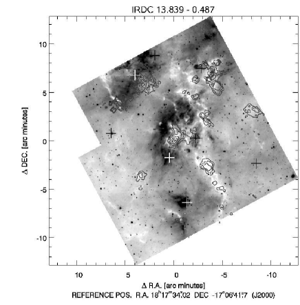
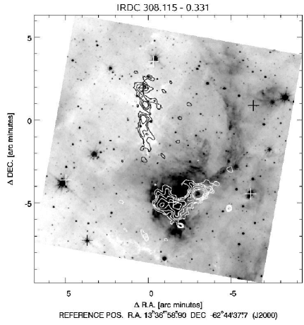
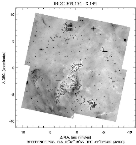
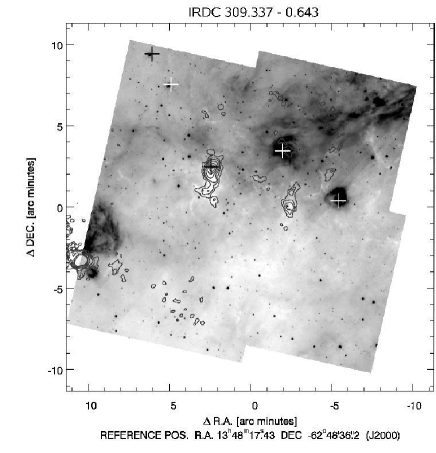
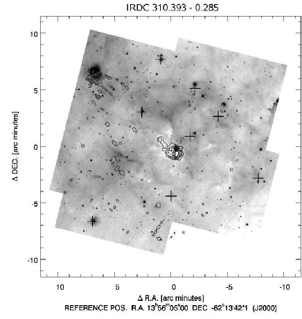
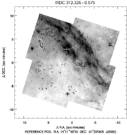
Figure 1: Inverse grey-scale 8 micron maps overlaid with 1.2 mm continuum emission. The intensity of a grey-scale image corresponds to the square root of the inverse intensity in mJy. The contours are 60, 108, 156, 240, 360, 480 mJy beam^-1 in all cases. Crosses denote the position of IRAS point sources.

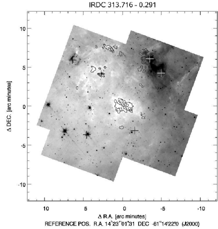
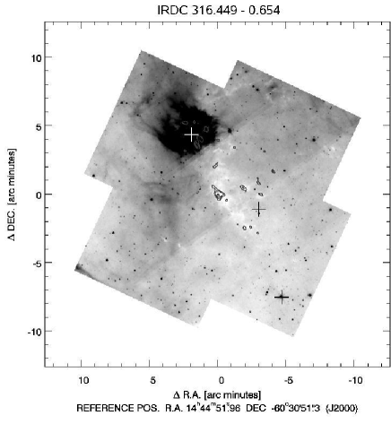
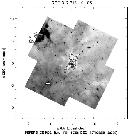
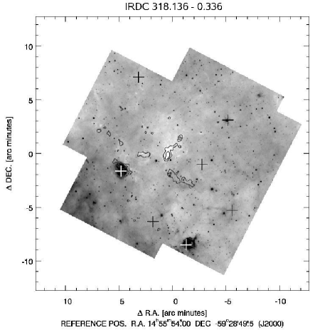
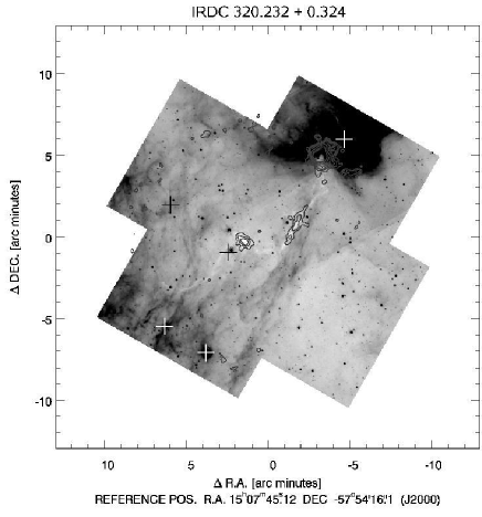
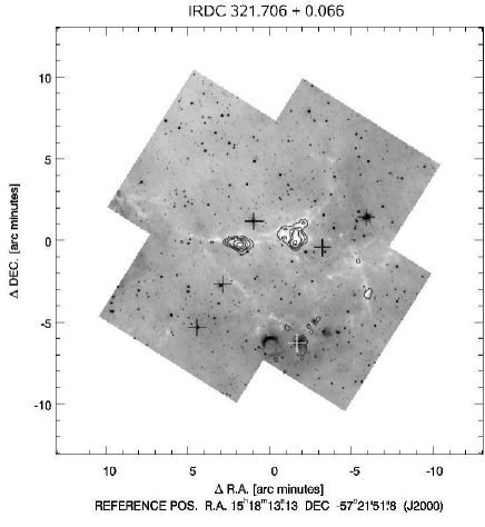
Figure 2: Inverse grey-scale 8 micron maps overlaid with 1.2. mm continuum emission. The intensity of a grey-scale image corresponds to the square root of the inverse intensity in mJy. The contours are 60, 108, 156, 240, 360, 480 mJy beam^-1 in all cases except for IRDC 316.45-0.65 where it is 84, 120, 156, 240, 360, 480 mJy beam^-1. Crosses denote the position of IRAS point sources.

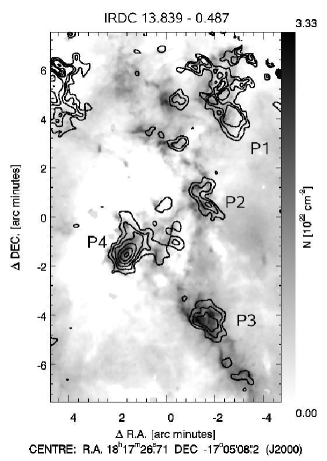
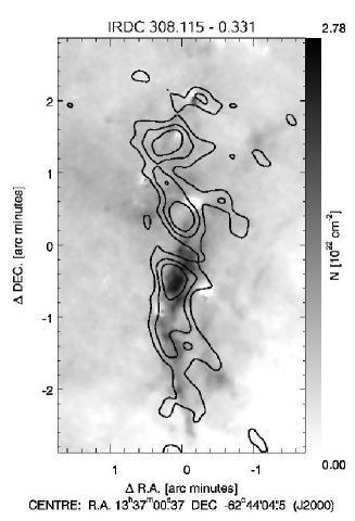
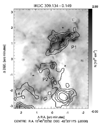
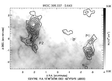
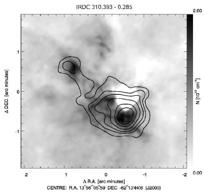
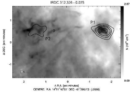
Figure 3: Column density maps derived from 8$\ \mu$m extinction overlaid with 1.2 mm continuum emission as contours. The scaling is indicated in the bar to the right of each image. The contours are 60, 108, 156, 240, 360, 480 mJy beam^-1 in all cases.

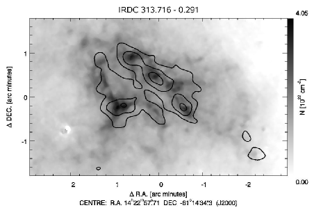
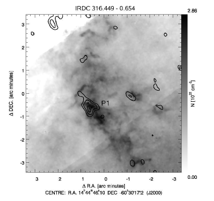
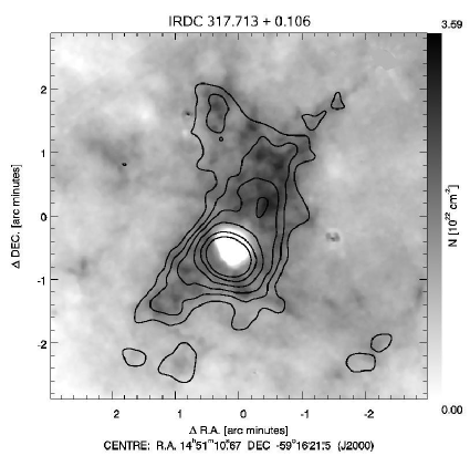
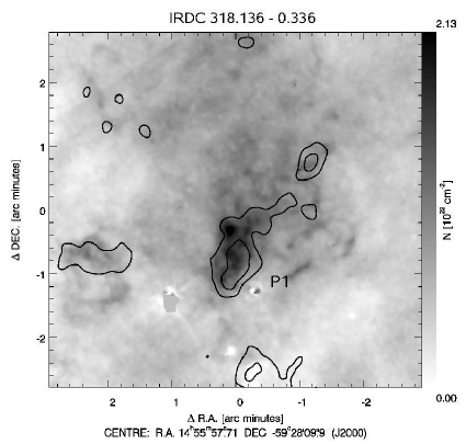
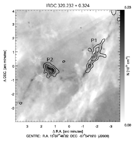
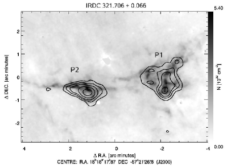
Figure 4: Column density maps derived from 8$\ \mu$m extinction overlaid with 1.2 mm continuum emission as contours. The scaling is indicated in the bar to the right of each image. The contours are 60, 108, 156, 240, 360, 480 mJy beam^-1 in all cases except for IRDC 316.45-0.65 which is 84, 120, 156, 240, 360, 480 mJy beam^-1.

3.2 GLIMPSE 8 $\mu$m data

The original selection of the IRDCs has been done still based on MSX images. In the meantime, the Spitzer satellite has succeeded MSX and provides much higher spatial resolution and sensitivity. GLIMPSE images for our regions with a pixel size of 0$\aas@@fstack{\prime\prime}$6 were retrieved from the NASA/IPAC Infrared Science Archive (IRSA) and re-mosaicked to cover the final field of our 1.2 mm maps of typically $15^{\prime}\times 15^{\prime}$ in order to get a picture of the IRDCs in relation to their closer and further vicinity (see Figs.  1–2). After bad pixel removal, a PSF photometry has been performed using the STARFINDER program (Diolaiti et al. 2000). This allows to remove compact foreground objects, and thus maps of extended emission and absorption structures and finally column density maps could be extracted in a subsequent step.

Dust masses for the IRDCs were computed assuming that they are in the foreground and shadow emission from behind. The optical depth $\tau$ is ideally the logarithm of the ratio of two fluxes: (a) the flux from the emission background $I_{\rm back}$ directly behind the IRDC, and (b) the actually measured remnant flux $I_{\rm IRDC}$ from the location of the IRDC. Furthermore, superimposed on the IRDC is an emission contribution from foreground material, $I_{\rm fore}$, which has to be subtracted. Since $I_{\rm back}$ cannot be directly estimated we need a measurable quantity $I_{\rm 0}$ that can be used as a proxy for $I_{\rm back}$. Then the optical depth is given by

$$\tau=\ln\left(\frac{I_{\rm 0}-I_{\rm fore}}{I_{\rm IRDC}-I_{\rm fore}}\right)$$ (3)

Following Peretto et al. (2008) we assume that $I_{\rm fore}$ = $I_{\rm zl}$, where $I_{\rm zl}$ is the zodiacal light, which is systematically calculated for every Spitzer observation and available in the image header. For the quantity $I_{0}$ we used the average emission level from a patch of MIR emission in the close vicinity of the actual cloud. These emission patches, typically around 1 square arcminute in size, were chosen manually in order to capture the characteristic emission level for the background approximation of the individual clouds and to exclude strong compact emission sources. The mean and standard deviation of the emission levels within these defined regions have been computed in order to be used as $I_{0}$ in Equ. 3. The standard deviation obtained here is propagated through the following steps and is used to give formal errors for the derived masses and column densities, as listed in Table 3.

After optical depth determination, this quantity is converted into column densities and finally to masses by using the following equations:

$$N_{\rm H_{2}}=1.086\frac{\tau}{\sigma},$$ (4)

$$M={\rm m}_{\rm H_{2}}\ \ A\ \ N_{\rm H_{2}},$$ (5)

where $N_{\rm H_{2}}$ is the H₂ molecule column density, m${}_{\rm H_{2}}$ is the mass of one hydrogen molecule, and $A$ is the area per pixel. $\sigma$ is the extinction cross section per hydrogen molecule. According to the adopted dust extinction model by Weingartner & Draine (2001, see below), $\sigma=4.62\times 10^{-23}\,{\rm cm}^{2}$ for the Spitzer/IRAC band 4 central wavelength of 7.87 $\mu$m.

The derived masses critically depend on the used extinction–column density calibration, the distance to the targets, and the method to select the relevant extinction regions. As dust model we used the parametrisation of Weingartner & Draine (2001) according to their model B with R_V = 5.5. This particular model has been shown to be relevant for massive star–forming regions, e.g., by Indebetouw et al. (2005). It differs from the common dust models (e.g., Draine & Lee 1984) in that it predicts higher extinction cross sections especially in the 4–8 micron wavelength region, a relevant point for the Spitzer extinction maps. We note in passing that such elevated cross sections are also predicted in connection with ice-coated dust grains and especially if dust coagulation processes are involved (Ossenkopf & Henning 1994). The chosen dust model finally relates the optical depth (and, equivalently, the extinction magnitude at the used wavelength) to the equivalent column density of hydrogen molecules. The quadratic dependence of the masses on the distance is in the extinction map case the same as for masses derived from the 1.2 mm emission data.

Table 1: Comparison of the 1.2 mm emission and 8 $\mu$m absorption techniques for deriving masses and column densities.

Properties	1.2 mm	8 $\mu$m
Distance dependencea	+	+
Resolution	24′′	3′′
Sensitive to lower column	-	+
density filigree structure
Temperature dependence	+	-
Background and foreground	not	necessary
estimation	necessary
Sensitive to column	+	-
densities $\gg 10^{23}$ cm-2

• Only for masses

Table 2: Comparison of the different observational techniques for IRDC 18223-3.

Data	Resolution	Column density	Optical depth	Contrast
	(arcsec)	(1022 cm -2)	at 8 $\mu$m	($\rm I_{bg}/I_{IRDC}$)
8 $\mu$m GLIMPSE	3	2.3	0.95	2.5
1.2 mm IRAMa	11	5.9	2.4	11
3.2 mm PdBIb	5$\aas@@fstack{\prime\prime}$8 $\times$ 2$\aas@@fstack{\prime\prime}$4	45	19	1.8e+08
1.3 mm SMAc	1$\aas@@fstack{\prime\prime}$3 $\times$ 1$\aas@@fstack{\prime\prime}$4	93	40	1.8e+17

• Beuther et al. (2002)

• Beuther et al. (2005)

• Fallscheer, Beuther, et al. 2009 in preparation

3.3 Comparison of techniques

Using the data from two different regions of the spectrum and two different techniques for estimating IRDC parameters, enables us to compare the results and to analyse advantages and disadvantages of both methods (see Table 1). The mid-IR data have an effective resolution of around 3^′′, which is much higher than 24^′′ for our millimeter data. The estimated total masses and peak column densities have no dependence on the temperature. On the other hand, when using 8 $\mu$m data to calculate the optical depth and then the column density in the cloud, we have to estimate the expected flux from the background indirectly. We assume the background flux as the difference between an average intensity around the cloud and the foreground intensity, but in reality matter hidden by the infrared dark cloud can be inhomogeneous and has either lower or higher intensity. However, the logarithm in Eq. (3) to a certain degree mitigates uncertainties in the estimation of the intensities necessary for evaluating Eq. (3).
Simon et al. (2006a) have used an automated approach where they strongly smooth the original (MSX) mid-infrared images and basically use these smoothed data as approximation for the quantity $I_{0}$ (cf. Eq. 3). We tested this approach for one of our clouds but found that unless very large smoothing kernels are used, the herewith derived intensity contrasts are systematically smaller than for the method we employed (Sect. 3.2). For very large smoothing kernels ($>10^{\prime}$) it is very difficult to control the process. Continuum emission from strong extended emission sources in the surroundings might be folded into the area of the IRDCs, depending on the individual circumstances. Therefore, we refrain from using this smoothing approach in order to have better control for the estimation of the quantity $I_{0}$.
Uncertainties in the foreground level estimation also affect the resulting masses and column densities. At the moment we take into account only the zodiacal light contribution, which typically accounts for 15%–20% of the intensity toward the IRDCs. An extreme (hypothetical) case may be, that all remaining flux received from the IRDC, down to the noise level $I_{\rm noise}$ of the GLIMPSE images, is produced by another foreground emission contribution (e.g., the PDR surface of the cloud, glowing in PAH emission). After removing all this emission down to $I_{\rm noise}$, the resulting intensity contrast would of course be clearly higher. However, considering typical levels for $I_{\rm noise}$ and $I_{\rm Back}$, our results for the column densities would rise just by a factor of around 3. This is again due to the alleviating effect of the logarithm in Eq. (3), acting on the intensity contrast.

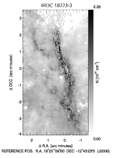
Figure 5: Column density map derived from an 8$\mu$m Spitzer/GLIMPSE image overlaid with 1.2 mm IRAM continuum emission as contours. The image scaling is indicated in the sidebar. The contours are 38,76,114,190,266 mJy beam^-1. The (0,0) position corresponds to the center of the IRDC 18223-3.

While for almost all our clouds peak column densities extracted from the GLIMPSE data are slightly higher than the values derived from the millimeter data, this difference does not correspond to the factor 8 in resolution. Therefore, we made a comparison between the peak column densities, extracted from different observational data for the previously studied IRDC 18223-3 (Beuther et al. 2002, 2005), which is located 3.7 kpc from us and has a NH₃ rotation temperature of $\sim$ 33 K (Sridharan et al. 2005). For this particular cloud, 1.2 mm IRAM single-dish observations (Beuther et al. 2002), 8 micron Spitzer/GLIMPSE data and interferometric data at 3.2 and 1.3 mm data obtained with the PdBI and SMA (Beuther et al. 2005, Fallscheer et al. 2009 in prep.) are available, with the spatial resolution ranging from 11 arcsec down to 1.4 arcsec (Table 2). For the GLIMPSE data we obtained a column density distribution map according to the algorithm described in Sect. 3.2. Together with the 1.2 mm IRAM data as contours, this result is presented in Fig. 5. The peak column densities for all the millimeter data were calculated using Eq. (2), adopting the different beam sizes. Always a temperature of 33 K (Sridharan et al. 2005) has been used. The peak flux density for the 3.2 mm PdBI data we took from the corresponding paper (Beuther et al. 2005), while we (re-)assessed the peak flux densities for the IRAM and SMA data on the related FITS files, kindly provided by H. Beuther and C. Fallscheer. For the dust opacity per gram of dust, as for our SIMBA millimeter data, we have always used the same opacity model, appropriate for coagulated dust particles with thin ice mantles (Ossenkopf & Henning 1994, opacity column 5 in their Table 1). As we can see in Table 2, the peak column density derived from the high-resolution millimeter interferometry data is a factor of 40 higher than the one extracted with the mid-IR technique. A factor of a few between the mid-infrared and the millimeter single-dish results for the peak column densities can be accounted for by using other dust opacities/extinction cross sections or more extreme assumptions on the MIR foreground contribution (see above). However, the large difference between the mid-infrared and the millimeter interferometry results indicates a principle limitation of the extinction method to distinguish high column density peaks. The realistically attainable intensity contrast at high optical depths sets this limit. In Table 2, we list the optical depths and image contrasts at 8 micron that would correspond to the column densities derived from the millimeter data. Obviously, realistic 8 micron images cannot provide such humongously high dynamic ranges necessary to derive column densities similar to the interferometry results.

4 Results

4.1 Morphology of the IRDCs

The morphology of the clouds in our sample ranged from compact structures (IRDC 312.33-0.07 P1 and P2) to filaments (IRDC 309.13-0.15). They have sizes from 1^′ (IRDC 013.84-0.49 P2 and P3) to 4^′ (IRDC 317.71+0.11), which roughly corresponds to 1–3.5 pc at the distance of these clouds. There is, in general, a good agreement between the morphologies of the 1.2 mm emission and the 8 $\mu$m extinction structures (see Fig. 3-4). As a rule, dense areas of extinction material (IRDCs 013.84-0.49, 313.72-0.29 etc.) coincide with relatively bright compact sources at 1.2 mm. For some IRDC complexes, some emission peaks at the millimeter wavelengths are associated with mid-IR emission sources (IRDCs 309.13-0.15 P2, 309.34-0.64 P2 and 317.71+0.11) which indicates later evolutionary stages than those objects corresponding to 8 micron extinction. Among all clouds there is one particular case - IRDC 310.39-0.28, where the millimeter emission still peaks at the extinction maximum despite the existence of a bright MIR emission source nearby. The IRDCs 013.84-0.49, 312.33-0.07, 318.13-0.34, 320.23+0.32, and 321.71+0.07 present several separated sources at mm wavelengths, which coincide with dense 8 $\mu$m features. IRDC 308.12-0.33 has an elongated shape and three sub-structures can be recognized, one of them corresponds to the extinction maximum at mid-IR wavelengths. IRDC 309.13-0.15 shows two distinct 1.2 mm emission sources: the compact object (P1) coincides with the MIR extinction region, another one (P2) has an emission peak corresponding to the 8 $\mu$m emission and an elongated ”tail”. Extended millimeter emission, 2${}^{\prime}\times 4^{\prime}$ in size, with at least four sub-structures is present in IRDC 313.72-0.29. For IRDC 316.45-0.66, we can recognise only one weak 1.2 mm source and diffuse extended MIR extinction structures.

Positions of known IRAS sources are marked with plus-signs on the Figs. 1–2, where the IRAC 8 $\mu$m data are displayed as inverse grey-scale images, and contours present the 1.2 mm data. As a rule IRAS sources do not correspond to the extinction regions at 8 $\mu$m. On the contrary, they agree with the locations where MIR emission coincides with millimeter emission peaks or just with the very bright MIR emission sources. In the case of IRDC 317.71+0.11, the kinematic distance to one of the IRAS sources, located in the center of the 8 $\mu$m emission, can be derived using the CS (2–1) line velocities reported by Bronfman et al. (1996) toward this IRAS source. The $v_{\rm LSR}$ velocities of this CS measurement and our HCO⁺ data for the neighbouring IRDC are less than 0.5 km/s different. The distance to the cloud and the IRAS source is then around 2.9 kpc. Hence, assuming that the dark cloud is related with this IRAS point source, the infrared luminosity of the compound (IR source + IRDC) is $\approx$ 10⁴ L_⊙, using the IRAS approximation formula from Henning et al. (1990). This is the typical order of magnitude for pre-main-sequence OB stars.

4.2 Masses and column densities

Toward all 12 clouds millimeter continuum emission was detected and column density maps were extracted from 8 $\mu$m images according to the algorithm described in Sect. 3.2. Figures 3-4 present these column density maps for every region, superimposed with the corresponding 1.2 mm contours. In Table 3 the properties of the IRDCs are compiled: name, right ascension, declination, distance, peak flux density and integrated flux density, mass and peak column density of the 1.2 mm sources, mass and peak column density of the extinction matter. For every cloud in the table, the first line corresponds to the total millimeter flux density as well as total masses of the emission and extinction matter. The following lines present data for the separate millimeter sub-clumps which are labeled with ”P”.

Where appropriate, we distinguished separate sub–clumps at 1.2 mm. In the Fig. 3-4 and in Table 3 these separate emission sources are named with the designation ”P” (e.g. P1, P2). For all of them we measured peak flux density and integrated flux density, derived masses and column densities according to Equ. 1 - 2. In the case of IRDCs 309.13-0.15 (P2), 309.34-0.64 (P2) and 317.71+0.11 (P1) parts which coincide with strong 8 $\mu$m emission features were not taken into account for measuring 1.2 mm flux densities and hence for estimating masses and column densities. The typical range of masses of the separate millimeter sources with $T$ = 20 K is 50-1000 $\rm M_{\odot}$, and the column densities range between 0.9 and 4.6 $\times 10^{22}$ cm^-2.

For calculating total masses of the extinction material in individual clumps we took regions above 3 sigma into account, where sigma is in this case the standard deviation in the full extinction maps. The total masses of the IRDCs for extinction matter were found to range from 300 to 1700 $\rm M_{\odot}$ and the derived peak column densities correspond to values from 2.1 to 5.4 $\times 10^{22}$ cm^-2.

Table 3: Properties of the IRDCs. For every cloud the first line corresponds to the total mass, the following to the masses of separate millimeter sources.

Name	R.A.	Decl.	D	Peak Flux density	Integrated Flux density	Mass 1.2mm	N (1.2 mm)1	N0 (1.2 mm)2	Mass (8 $\mu$m)	N (8 $\mu$m)
	(J2000.0)	(J2000.0)	(kpc)	(mJy)	(Jy)	($\rm M_{\odot}$)	(1022 cm -2)	(1022 cm -2)	($\rm M_{\odot}$)	(1022 cm -2)
IRDC 308.12$-$0.33	13 37 01.2	$-$62 44 40	4.32	225	1.88	580	1.7	60.3	520${}^{+40}_{-30}$	2.8${}^{+0.16}_{-0.16}$
IRDC 309.13$-$0.15	13 45 17.1	$-$62 21 57	3.92	3303	4.393	11503	2.63		1750${}^{+370}_{-310}$	3.0${}^{+0.13}_{-0.13}$
P1				162	1.37	360	1.3	41.9
P2				124	0.96	250	0.9
IRDC 309.34$-$0.64	13 48 39.8	$-$62 47 26	3.46	5043	3.693	7503	3.93		750${}^{+170}_{-150}$	3.1${}^{+0.24}_{-0.24}$
P1				216	0.94	190	1.7	48.5
P2				155	0.81	170	1.3
IRDC 310.39$-$0.28	13 56 01.7	$-$62 14 27	4.93	594	2.48	1029	4.6	186.1	1320${}^{+60}_{-50}$	2.6${}^{+0.16}_{-0.16}$
IRDC 312.33$-$0.07	14 11 56.8	$-$61 29 25	4.05	288	0.77	210	2.3	76.6	290${}^{+100}_{-60}$	2.7${}^{+0.33}_{-0.16}$
P1				288	0.46	130	2.3
P2				92	0.31	90	0.7
IRDC 313.72$-$0.29	14 23 05.4	$-$61 14 48	3.33	172	1.98	370	1.3	35.7	700${}^{+90}_{-70}$	4.1${}^{+0.16}_{-0.16}$
IRDC 316.45$-$0.66	14 44 50.4	$-$60 30 54	3.01	159	0.96	150	1.3	32.3	430${}^{+80}_{-70}$	2.9${}^{+0.16}_{-0.16}$
P1				159	0.58	90	1.3
IRDC 317.71$+$0.11	14 51 07.5	$-$59 16 11	2.9	9543	8.003	11503	7.53		1320${}^{+150}_{-150}$	3.6${}^{+0.15}_{-0.15}$
P1				250	1.98	280	2.0	47.9
IRDC 318.13$-$0.34	14 55 58.4	$-$59 28 31	2.96	142	2.48	370	1.1	26.9	680${}^{+160}_{-140}$	2.1${}^{+0.16}_{-0.16}$
P1				142	1.02	150	1.1
IRDC 320.23$+$0.32	15 07 56.7	$-$57 54 27	1.97	186	1.68	110	1.5	24.6	600${}^{+320}_{-250}$	5.2${}^{+0.16}_{-0.16}$
P1				142	1.00	70	1.1
P2				186	0.68	50	1.5
IRDC 321.71$+$0.07	15 18 26.7	$-$57 21 56	2.14	408	3.12	240	3.2	56.9	460 ${}^{+80}_{-80}$	5.4${}^{+0.16}_{-0.23}$
P1				276	1.69	130	2.2
P2				408	1.43	110	3.2
IRDC 013.84$-$0.49	18 17 21.2	$-$17 09 23	2.66	438	9.38	1130	3.5	77.0	1150${}^{+130}_{-120}$	3.3${}^{+0.13}_{-0.13}$
P1				214	2.97	360	1.6
P2				163	1.12	130	1.3
P3				192	1.45	170	1.5
P4				438	3.54	430	3.5

¹ Peak column density per beam

² Extrapolated column density, obtained by applying the correction factor explained in Sect. 4.3.2

³ This mm peak corresponds to a mid-infrared bright source near to the IRDC.

4.3 Comparison with results for other cores

In this chapter we will compare our results with previously obtained characteristics for low- and high-mass pre-stellar cores.

4.3.1 Comparison with low-mass cores

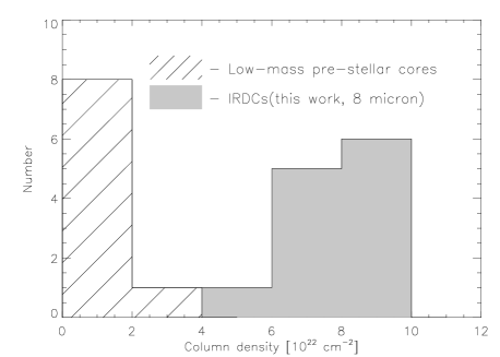
Figure 6: Histogram showing the principle distribution of column densities for a collection of low-mass cores from Bacmann et al. (2000) (after taking into account consideration (a) from Sect. 4.3.1) and for the IRDCs presented here (after taking into account consideration (b) from Sect. 4.3.1). The Mann-Whitney-U one-tailed test confirms the clear separation of the two distributions even when the different spatial resolutions (consideration (b)) are not taken into account (Sect. 4.3.1).

During recent years, extinction mapping has mainly been applied along the lines of the near-infrared colour excess method (e.g., Lombardi & Alves 2001; Lombardi 2008) or classical star count techniques in the visible or near-infrared (e.g., Dobashi et al. 2005; Froebrich et al. 2005). Such approaches are most powerful towards medium-extinction regions. In contrast, the extinction map method used in the current paper exploits the extinction of mid-infrared extended emission and hence does not rely on the identification of stellar background sources. This method can peak into cores having column densities of up to $10^{23}$ cm^-2 It has been used previously for the analysis of low-mass starless cores based on ISOCAM data (Bacmann et al. 2000) which gives us the opportunity to compare our results. To make a fair comparison, two effects have to be considered. (a) Bacmann et al. (2000) used the standard Draine & Lee (1984) extinction cross sections. These are more than a factor of 3 smaller than the Weingartner & Draine (2001) values we use. Therefore, we recomputed the peak column densities reported in Bacmann et al. (2000) for the low-mass cores by adopting the Weingartner & Draine (2001) dust extinction model. (b) For the low-mass cores, which typically reside at distances of less than 300 pc, the linear spatial resolution is much better than in the case of IRDCs with their distances of 2 - 5 kpc. Therefore, the actual column density peaks are much better resolved in the low-mass case. To assess the effect of poor spatial resolution on our derived peak column densities, we used a synthetic column density map derived in Steinacker et al. (2005) for one of the low-mass cores of Bacmann et al. (2000), namely Rho Oph D ($d$ = 160 pc). We convolved this map with kernels appropriate to emulate the much coarser linear resolution toward our IRDC targets and computed the ratio of the unsmoothed to the smoothed peak column density value. These factors (typically in the range from 1.5 to 3.5) have been multiplied to the peak column densities we have originally derived from the IRDC extinction maps.
A comparison of the column densities for low-mass cores and our IRDCs, after taking into account the just mentioned considerations (a) and (b), is shown in Fig. 6. Here we can see a clear trend for high-mass cores to attain higher column densities than the low-mass objects. This qualitative difference shows that IRDCs are not just far away Taurus-like clouds, but a distinct type of clouds with the potential to form a distinct type of stars (see below and Sect. 4.4).

It might be of concern that in step (b) we applied a correction factor which increases the column densities with increasing kinematic distance. To statistically fortify our statement that Infrared Dark Clouds present “stochastically larger” values for column densities than low-mass pre-stellar cores we used the (Wilcoxon)-Mann-Whitney U one-tailed test (e.g., Wall & Jenkins 2003). It is a non-parametric test for assessing whether two samples of observations come from the same distribution or not. It works well on a small number of observations in one sample. The null hypothesis is that the two samples are drawn from a single population. For the test we used low-mass column density values from Bacmann et al. (2000) adopted to the Weingartner & Draine (2001) dust extinction model and column densities for IRDCs without applying the linear spatial resolution correction (b) mentioned above.

For both populations we computed the Rank Sum within the nonparametric Mann-Whitney statistic, usually called U (108 vs 0). The distribution of the U-statistic under the null hypothesis is known and can be found in special tables (e.g., Siegel & Castellan 1988). Then, we estimated the probability that the values for low-mass objects and IRDCs came from the same distribution. The obtained probability lower than 0.005 rejects the null hypothesis and shows that our two samples come from different distributions.

4.3.2 Comparison with high-mass cores

The high-mass clumps we want to compare have all been observed at 1.2 mm, comprising the following samples: high-mass starless core candidates (HMSCs) (Sridharan et al. 2005; Beuther et al. 2002), Infrared Dark Clouds from Rathborne et al. (2006), and results presented in this paper for our 1.2 mm data. To (re-)calculate peak column densities for the first two sets of data we used Eq. (2) as well. In the case of HMSCs, peak flux densities were taken from Beuther et al. (2002), distance and temperature estimates for all these objects come from Sridharan et al. (2005). In Rathborne et al. (2006), for all 38 IRDCs peak flux densities and distances are presented. For the calculation, we assume again 20 K for the temperature, as dust opacity $\varkappa_{v}$ and gas-to-dust mass ratio we adopt the values 1.0 cm² g^-1 and 100, respectively. Hence, we use here the same parameters as for the analysis of our 1.2 mm data, except for the different beam size, equal to (11^′′)² in steradians, adapted to the IRAM 30-m telescope.

Still, the measured data are affected by the convolution with the observational beam, which results in different linear smoothing scales for objects at different distances. In order to eliminate this smoothing effect, we attempted to extrapolate the measured peak column densities per beam back to the true values, assuming an (analytic) column density profile. But what is an appropriate choice for such a power law? A first idea is to use the data at different beam sizes we have for IRDC 18223-3 (Sect. 3.3). However, it turns out that these data sets give no unique trend for such a power law. The comparison between the IRAM 30-m data and the SMA data speak for a relatively steep power law of $N\sim$ r^-1.75, and the comparison with the PdBI data would even indicate a much steeper power law index. The fact that these two data sets do not result in a similar power law may be related to the different degree these observations are able to recover extended emission. Furthermore, at the high spatial resolution of the SMA observations, we begin to see a dense rotation structure (Fallscheer et al. 2009, in prep.) that is distinct from the rest of the surrounding clump. However, we also compared the column density values for a few other IRDCs, observed both at single-dish and interferometric resolution (Rathborne et al. 2006, 2008). Again, no clear trend for a certain power law range is obvious. According to Johnstone et al. (2003), for the filament structure of the famous IRDC G11.11-0.02 the column density profile should be very steep and may reach $\sim$ r^-3. Such a significant difference to commonly observed values might be an additional feature characterizing massive star forming clumps, especially if filamentary structures are involved. On the other hand, Bacmann et al. (2000) showed that N $\sim$ r^-1 can be a reasonable choice for lower-mass starless cores, and also the single dish mapping of young massive clumps by Beuther et al. (2002) resulted in less steep power laws for the column density quite close to the low-mass core results. Hence, by assuming N $\sim$ r^-1 for the extrapolation to the true column densities will provide us with a kind of robust lower limit.

To recalculate all column density values, an artificial column density distribution map was created (by just assuming an analytical N $\sim$ r^-1 profile) with the peak in the centre of the array normalised to 1.0 and the assumption that 1 pixel corresponds to 2000 AU (a typical size scale for fragmentation). Then, for every source from the three high-mass samples mentioned above, this column density distribution map has been convolved with a smoothing Gaussian kernel emulating the effect of observing at mm wavelengths with single-dish telescopes (11–24^′′ beam). The kernel size (FWHM) is computed by taking the ratio of the effective linear resolution (in AU) achieved within the observed mm maps and the 2000 AU pixel size from the artificial map. After convolving the artificial map with such a Gaussian kernel, the peak column densities in these synthetic maps are smaller than 1. The correction factor for every source is then the ratio of the original peak column density value (1.0) to the peak column density value after beam convolution. These factors are then applied to the column density values derived according to the Eq. (2), which then approximates the true peak column density values. These extrapolated values for the new regions reported here are also given in column 9 of Table 3.

Figure 7 summarizes the distribution of the extrapolated peak column densities we have finally obtained. The distribution of the true peak column densities indicates a similar order of magnitude for previously obtained values for the two other samples of massive star forming regions and our new SIMBA results. Most of the clouds have (extrapolated) column densities in the range from 1.0 to 12.0 $\times 10^{23}$ cm^-2 with few exceptions reaching 20.0 - 30.0 $\times 10^{23}$ cm^-2.

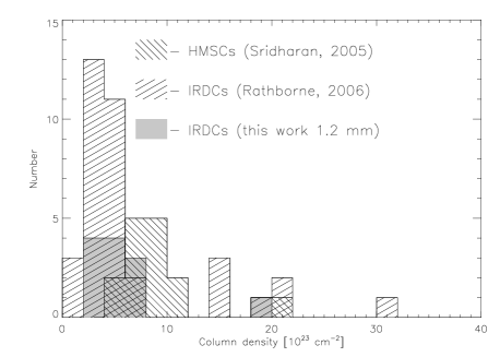
Figure 7: Distribution of extrapolated column densities for the HMSCs from Sridharan et al. (2005), the IRDCs from Rathborne et al. (2006), and the IRDCs from the present paper. Note that we have applied the corrections and extrapolations mentioned in Sect. 4.3.2 for all these high-mass cores.

4.4 Comparison with theoretical models.

Infrared Dark Clouds, located several kpc away from us, have large masses, volume and column densities, but “high” values alone do not guarantee that they are really the progenitors of massive stars, and we need additional criteria to estimate this possibility. According to Krumholz & McKee (2008) only clouds with column densities of at least 1 g cm^-2, which corresponds to 3 $\times 10^{23}$ cm^-2 in our units, can form massive stars. As we can see in Table 3, the direct transformation of observational results for IRDCs from our list indicates peak column densities one order of magnitude lower than this limit. On the other hand, as it was shown in Sect. 4.3, that the directly observed peak column densities are still affected by the convolution with the beam of the millimeter observations. After taking this into account, the derived values for the extrapolated column density rise by a factor of 10 or higher (see Fig. 7). Thus, we can reach the 3 $\times 10^{23}$ cm^-2 threshold in the case of the infrared dark clouds.

Since we have not only compact sources, but also very filamentary structures like IRDC 320.23+0.32 P1, this raises the question, whether it is possible to form massive stars in such structures. Banerjee & Pudritz (2008) showed that filaments play a dominant role in controlling the physics, accretion rate, and angular momentum of the much smaller-scale accretion disk that forms within such collapsing structures. Large-scale filamentary flows sustain a very high accretion rate ($\dot{M}\sim$ 10${}^{-2}\ \rm M_{\odot}\$yr^-1) due to the supersonic gas flow onto the protostellar disk. These rates are 10³ times larger than predicted by the collapse of the singular isothermal spheres and exeed the accretion rates necessary to squeeze the radiation field of the newly born massive star. Thus, for almost all our clouds we still see the potential to form massive stars.

5 Conclusions

In this paper, we discuss our progress in understanding properties of Infrared Dark Clouds. A set of 12 clouds located in the southern hemisphere has been selected from the MSX 8.3 micron images. For these clouds 1.2 mm maps were obtained with the SIMBA bolometer array at the SEST telescope. GLIMPSE mid-infrared images for these regions were retrieved from the Spitzer Archive.

The new sources comprise a variety of IRDC morphologies, from compact cores to filamentary shaped ones, from infrared quiet examples (no Spitzer 8 $\mu$m emission sources) to more active ones. As a rule, our sample shows a good agreement between the morphologies of 1.2 mm emission and 8 $\mu$m extinction features. The total masses of the IRDCs were found to range from 150 to 1150 $\rm M_{\odot}$ (emission data) and from 300 to 1750 $\rm M_{\odot}$ (extinction data). We derived peak column densities between 0.9 and 4.6 $\times 10^{22}$ cm^-2 (emission data) and 2.1 and 5.4 $\times 10^{22}$ cm^-2 (extinction data).

Since the MIR extinction method has been used previously for the analysis of low-mass starless cores we check how our findings relate to the published results. To make a fair comparison, we used the same dust model and the same spatial resolution in both cases. It is shown, that there is a clear trend for the high mass cores to attain higher column densities than the low-mass objects. This qualitative difference means that most IRDCs are not just far away Taurus-like clouds, but a distinct type of clouds with the potential to form a distinct type of stars. A simple statistical analysis (the Mann-Whitney-U one-tailed test) confirms this statement also when the different spatial resolutions are not taken into account and thus the IRDC column densities are underestimated.

Using the data from two different regions of the spectrum and applying two different techniques for estimating IRDC parameters enables us to compare these two methods. On the one hand, the extinction technique has some advantages over the millimeter technique. It is a ”cheap” method since GLIMPSE at 8 $\mu$m has covered large parts of the Galactic plane in the 4th and 1st quadrant. The GLIMPSE data have a better spatial resolution than millimeter single-dish data, which reveals the often filigree substructures of the clouds. Furthermore, this method does not depend on assumptions for the temperature of the IRDCs for estimating masses and column densities. However, our comparison shows, that the extinction method has a principle limitation to distinguish very high image contrasts and hence to find high column density peaks $\gg 10^{23}$ cm^-2. Hence with the extinction method we can give only a lower limit to the column density values, inspite of high resolution. The limit is around $A_{\rm V}=75$ mag when applying the Weingartner & Draine (2001) $R_{\rm V}=5.5$ B extinction law (corresponding to roughly 200 mag when following the common $R_{\rm V}=3.1$ extinctionlaw reviewed in Mathis 1990). High-spatial resolution (sub-)millimeter observations are hence crucial to assess even higher column density ranges and to reveal the actual column density maxima.

To compare column densities extracted with the emission method with previously obtained values for IRDCs and HMPOs, we extrapolated them back to the true peak column densities by assuming a column density profile $\sim$ r^-1, thus, mitigating the spatial resolution differences within the different samples. The distribution of the true peak column densities indicates a similar order of magnitude for our new SIMBA results and the two other samples of massive star forming regions. Moreover, the true peak column densities exceed the theoretical limit of 3 $\times 10^{23}$ cm^-2 (or 1 g cm^-2), recently put forth to distinguish potentially high-mass star-forming clouds.

Thus, extracted values for masses and column densities both for emission and extinction matter show a clear difference between IRDCs and known low-mass pre-stellar cores, and confirm our assumptions that Infrared Dark Clouds can present the earliest stages of high-mass star formation.