An analytic column density profile to fit prestellar cores

Abstract

We present a new analytical three-parameter formula to fit observed column density profiles of prestellar cores. It represents a line-of-sight integral through a spherically symmetric or disc-like isothermal cloud. The underlying model resembles the Bonnor-Ebert model in that it features a flat central region leading into a power-law decline $\propto r^{-2}$ in density, and a well-defined outer radius. However, we do not assume that the cloud is in equilibrium, and can instead make qualitative statements about its dynamical state (expansion, equilibrium, collapse) using the size of the flat region as a proxy. Instead of having temperature as a fitting parameter, our model includes it as input, and thus avoids possible inconsistencies. It is significantly easier to fit to observational data than the Bonnor-Ebert sphere. We apply this model to L1689B and B68. We show that L1689B cannot be in equilibrium but instead appears to be collapsing, while our model verifies that B68 is not far from being a hydrostatic object.

1 Introduction

In recent years, observational advances have made it possible to measure column density profiles in prestellar cores. Various methods are being used in the literature. Ward-Thompson, Motte, & André (1999) measured mm continuum emission, while Bacmann et al. (2000) utilized mid-IR absorption, and Alves, Lada, & Lada (2001) measured dust extinction and reddening of the light of background stars in the near-IR. A fourth method is to use flux measurements in optically thin lines (Tafalla et al., 2002). Most of the column density profiles measured in these ways show certain prominent common features: a central flat region, followed by a power-law decline. Some cores additionally exhibit signatures of steepening of the profile, while some show a more-or-less smooth merger to some background value of the column density (Bacmann et al., 2000).

One model often used to fit to such cores (e.g., Evans et al., 2001; Teixeira, Lada, & Alves, 2005) is the Bonnor-Ebert sphere (hereafter BE sphere). This model assumes an isothermal sphere in equilibrium, acted upon only by gravity and thermal pressure, and bound by some external pressure (Bonnor, 1956; Ebert, 1955). In the central region its density profile is flat with density $\approx\varrho_{\mathrm{c}}\equiv\varrho\left(r=0\right)$. The size of this region is proportional to the Jeans length, $R_{\mathrm{J}}\propto c_{\mathrm{s}}/\sqrt{G\varrho_{\mathrm{c}}}$. It transitions into a power-law decline that approaches the Singular Isothermal Sphere (SIS) with $\varrho_{\mathrm{SIS}}=c_{\mathrm{s}}^{2}\left(2\pi Gr^{2}\right)^{-1}$ for large radii (Shu, 1977). The cloud is finally cut off at some finite radius, where external pressure forces match the internal forces. The BE model invokes the dimensionless radius parameter $\xi\equiv r\sqrt{4\pi G\varrho_{\mathrm{c}}}/c_{\mathrm{s}}$. The value $\xi_{\mathrm{crit}}=6.45$ marks a dividing line such that clouds truncated at dimensionless radius $\xi_{\mathrm{s}}>\xi_{\mathrm{crit}}$ are in an unstable equilibrium, and clouds with $\xi_{\mathrm{s}}<\xi_{\mathrm{crit}}$ are stable.

The column density profile of the BE sphere, obtained by integrating the volume density numerically along a line of sight, matches well with some observations (B68; Alves et al., 2001). Depending on the parameters, the power-law decline $\propto r^{-1}$ in column density can be more or less pronounced, or even almost completely absent. The profile steepens at the edge because the line of sight through the sphere becomes shorter. This is a geometric effect which is present in all truncated models, unless the density increases sufficiently fast with radius.

While physically motivated and reproducing features of several observed column density profiles, the BE model has shortcomings. The most important is the key assumption of equilibrium. In fact, most fits are found to be supercritical (Teixeira et al., 2005), representing unstable equilibria. These states are not expected to exist in reality, as any perturbation will send them to immediate collapse. On a more practical side, the procedure of fitting the BE model to observations is quite involved. The volume density is only available as a numerical solution, which then needs to be integrated (again numerically) to calculate the column density. Sometimes the fit demands temperatures well above those measured for the centres of prestellar cores (Bacmann et al., 2000; André et al., 2003; Kirk, Ward-Thompson, & André, 2005), and predicted by detailed models of the thermodynamics within the core (Galli, Walmsley, & Gonçalves, 2002). Finally, most of the observed cores are deeply embedded within their parent clouds, and the source of a bounding external pressure is not obvious. The often-cited example B68 (Alves et al., 2001) is an exception, as it is thought to lie within a hot HII region.

We stress that the generic features of the BE density profile are not unique to equilibrium situations (see Kandori et al., 2005). The flat region with adjacent $r^{-2}$ density profile appears also in solutions of the hydrodynamic equations for gravitationally collapsing objects (Larson, 1969), as long as pressure is not completely negligible (Shu, Adams, & Lizano, 1987). The pressure gradient then establishes a region where it nearly balances gravity. Here, the density is nearly constant on the scale of the local Jeans length, shrinking in size over time as the density increases. Inverted, this requires that $\varrho\propto r^{-2}$ in the outer profile that is left behind outside the central region (see Basu, 1997).

There is no reason why the above two features (flat region with size of Jeans length and adjacent $r^{-2}$ density profile) should be present in a non-self-gravitating cloud. However, Ballesteros-Paredes, Klessen, & Vázquez-Semadeni (2003) find that convergent turbulent flows, with and even without self-gravity (which are expected to have very different volume density profiles), nevertheless yield column density profiles that resemble those of a BE sphere. There are three reasons for this seemingly surprising result. The first one is the effect of smoothing the data, by angle-averaging, and also by integration along the line of sight. Secondly, the BE sphere leaves the modeller the freedom to fit the size of the central flat region by varying the temperature. Indeed, Ballesteros-Paredes et al. (2003) fit their simulated cores with BE temperatures in the range of $5-60~{}\mathrm{K}$, despite their models being strictly isothermal at $T=11.3~{}\mathrm{K}$. Finally, the position of the outer radius cutoff is somewhat arbitrary. This often leaves large parts of profiles unfitted. In this paper, we argue that fitting a prestellar core profile at a set temperature does still allow one to distinguish between different models of internal structure.

We propose an analytic density profile reproducing the characteristics of not only isothermal equilibria (Bonnor, 1956; Ebert, 1955), but also non-equilibrium collapse solutions (e.g., Larson, 1969), and many observed profiles (Bacmann et al., 2000). Within the margins of uncertainty it fits the observations as well as the BE model does. However, it possesses a closed-form expression for the column density, and is therefore very easy to fit. Furthermore, the temperature can be an input parameter instead of a fitting parameter, so that the model avoids some of the possible inconsistencies of fitting the BE model to either observations or simulation results. We can use our model to make some inference about the dynamical state of the core.

This paper is organized the following way: Section 2 describes the spherical model and its parameters, while Section 3 presents a corresponding model for intrinsically flattened objects. In Section 4, we apply our model to B68 and L1689B, and we summarize our results in Section 5.

2 Spherical Geometry

2.1 Basic model

The characteristics found in observed column density profiles and theoretically both in equilibrium and collapse solutions can be parametrized by a volume density more generic than the BE sphere. We propose using the profile

$$\varrho\left(r\right)=\left\{\begin{array}[]{cc}\varrho_{\mathrm{c}}a^{2}/\left(r^{2}+a^{2}\right)&r\leq R,\\ 0&r>R,\end{array}\right.$$ (1)

characterized by a central volume density $\varrho_{c}$ and truncated at some radius $R$. The parameter $a$ fits the size of the flat region in terms of the Jeans length, and is given by

$$a=k\frac{c_{\mathrm{s}}}{\sqrt{G\varrho_{\mathrm{c}}}},$$ (2)

where $G$ is the gravitational constant and $k$ is a constant of proportionality. This profile is also mentioned in King (1962) and Tafalla et al. (2002). The temperature $T$, which can be constrained observationally, is not used as a fitting parameter. It enters through the value of the isothermal sound speed $c_{\mathrm{s}}=\sqrt{k_{\mathrm{B}}T/\mu}$. The Boltzmann constant is denoted by $k_{\mathrm{B}}$, and $\mu=2.33~{}m_{\mathrm{H}}$ is the mean mass of a particle, where $m_{\mathrm{H}}$ is the mass of a hydrogen atom. We assume a $10\%$ number fraction of helium.

The column density is derived by integrating the volume density along a line of sight through the sphere:

$$\Sigma\left(x\right) = 2\int_{0}^{\sqrt{R^{2}-x^{2}}}\varrho\left(s\right)ds$$ (3)

$$= 2\int_{x}^{R}\frac{\varrho\left(r\right)rdr}{\sqrt{r^{2}-x^{2}}}$$

where we have used the transformation $s=\sqrt{r^{2}-x^{2}}$ and hence $ds=rdr/\sqrt{r^{2}-x^{2}}$. Fig. 1 defines the quantities appearing in this derivation.

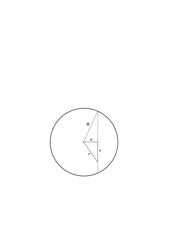
Figure 1: Schematic illustration of a cut through a spherical cloud of radius $R$. The observer is positioned along the direction of the coordinate $s$, and measures an integrated column density $\Sigma$ as a function of the offset $x$.

Inserting equation (1) into equation (3), we find that the integral is analytically tractable. The closed-form expression for the column density is then

$$\Sigma\left(x\right)=\frac{2a^{2}\varrho_{\mathrm{c}}}{\sqrt{x^{2}+a^{2}}}\arctan\left(\frac{\sqrt{R^{2}-x^{2}}}{\sqrt{x^{2}+a^{2}}}\right).$$ (4)

This can be re-written in terms of the central column density by introducing the ratio $c\equiv R/a$, called the concentration in King (1962). With $\Sigma\left(x=0\right)\equiv\Sigma_{\mathrm{c}}=2a\varrho_{\mathrm{c}}\arctan\left(c\right)$ we find

$$\Sigma\left(x\right) = \frac{\Sigma_{\mathrm{c}}}{\sqrt{1+\left(x/a\right)^{2}}}$$ (5)

$$\times\left[\left.{{\arctan\left(\sqrt{\frac{c^{2}-\left(x/a\right)^{2}}{1+\left(x/a\right)^{2}}}\right)}}\right/{\arctan\left(c\right)}\right].$$

Fig. 2 demonstrates that this profile possesses generic features that it shares with observations, collapse solutions, and with the BE model: a flat central region, a power-law decline, and steepening at the edge. We note that the effect of the boundary is exclusively contained in the factor in square brackets.

The quantity $c$ determines the size of the region described by the power-law. If it is large, there is a pronounced power-law, whereas if $c$ approaches unity, the cut-off already dominates near the flat region and inhibits the power-law.

Figure 2: Plots of equation (5) for varying $c\equiv R/a$. All cases have identical values for $a$. The central column densities are chosen to be different in order for the plots not to overlap. The solid line illustrates the three major characteristics of this function: the flat region in the centre of size $a$, the adjacent power-law decline $\propto x^{-1}$, a steepening at the edge for geometric reasons (see text), out to the cut-off radius $R$. In this case, $c=50$. The dashed-line shows a model dominated by the power-law regime, with $c>1000$. $R$ is chosen so that the influence of the cut-off is negligible. The long-dashed line finally demonstrates that the power-law can be suppressed entirely if $R\ga a$. In this case, $c=5$.

The three parameters to fit are (i) the outer radius $R$, (ii) the central column density $\Sigma_{\mathrm{c}}$, and (iii) the size of the flat region $a$. The latter contains the product of $k$ and $\sqrt{T}$, as shown in equation (2). If the temperature is pre-determined, $a$ only depends on the value of $k$. This then allows for a stability assessment, as demonstrated in the following section.

2.2 Model parameters

The pressure in an isothermal system is given by $P=c_{\mathrm{s}}^{2}\varrho$, and hence the pressure gradient for the spherically symmetric volume density profile of equation (1) is

$$\frac{dP}{dr}=c_{\mathrm{s}}^{2}\frac{d\varrho}{dr}=\frac{-2c_{\mathrm{s}}^{2}\varrho_{\mathrm{c}}r}{a^{2}\left[1+\left(r/a\right)^{2}\right]^{2}}.$$ (6)

In the inner regions, where $r\ll a$,

$$\frac{dP}{dr}|_{r\ll a}=\frac{-2c_{\mathrm{s}}^{2}\varrho_{\mathrm{c}}r}{a^{2}}.$$ (7)

This demonstrates a simple point: the larger the flat region $a$, the smaller the pressure gradient in that region. The minimal value for $a$ is reached in an equilibrium situation. A larger $a$ would result in a smaller pressure gradient, gravity would win out, and collapse would ensue. Conversely, for $a$ smaller than its equilibrium value the pressure force would dominate, causing expansion. However, that case is not probable since a profile with $\varrho\propto r^{-2}$ mandates a strong gravitational influence.

Another well-known model besides the SIS is the so-called Larson-Penston solution (LP solution), a self-similar spherical collapse solution, assuming a homogeneous initial density distribution (Larson, 1969; Penston, 1969). This highly dynamical model does not assume equilibrium, and asymptotically reaches a density profile for which

$$\varrho_{\mathrm{LP}}=4.4~{}\varrho_{\mathrm{SIS}}$$ (8)

everywhere. We now want to find an expression for the parameter $a$ in the SIS and the LP models. In the outer regions, equation (1) becomes

$$\varrho\left(r\gg a\right)\approx\frac{\varrho_{\mathrm{c}}a^{2}}{r^{2}}=\frac{\widetilde{k}c_{\mathrm{s}}^{2}}{2\pi Gr^{2}},$$ (9)

where $\widetilde{k}\equiv 2\pi k^{2}=1$ for the SIS (equilibrium) and $\widetilde{k}=4.4$ for the asymptotic LP collapse solution. Therefore

$$k\equiv\sqrt{\frac{\widetilde{k}}{2\pi}}=\left\{\begin{array}[]{cc}0.399&\text{for SIS},\\ 0.837&\text{for LP}.\end{array}\right.$$ (10)

This has a direct application to observed prestellar cores. If an estimate for the core temperature is available, equation (5) can be fit to the column density profile, with $k$ as a fitting parameter. If $k\approx 0.4$, the system can be considered to be in equilibrium. If $k$ is significantly larger than $0.4$, and closer to $1$, the cloud under scrutiny is collapsing.

Figure 3: Comparison between the BE sphere (dashed line) and our model (solid lines) for identical central temperature and cut-off radius. The top line is our model with $k=0.837$, for which the profile approaches the asymptotic LP solution. The lower line shows $k=0.399$, for which the SIS profile is reached. The dashed line represents the BE model, which also asymptotically approaches the SIS.

Fig. 3 shows our model with $a$ chosen to converge to either the SIS or the asymptotic LP solution. We also plot the equilibrium BE model. In order to avoid boundary effects, the outer radius was moved to $\approx 10^{2}~{}c_{\mathrm{s}}/\sqrt{G\varrho_{\mathrm{c}}}$. The BE profile does not join onto the SIS profile right away. It overshoots, then steepens and asymptotically approaches the SIS profile at large radii.

We may ask which value of $k$ is most appropriate to model a critical BE sphere. The overshoot effectively produces a larger flat region if the solution is truncated at $\xi_{\mathrm{s}}=\xi_{\mathrm{crit}}$. The resultant $a$ has to be larger than for the SIS. Having fixed the temperature this can only be achieved by increasing $k$, as we show in Fig. 4. Profile (a) shows a subcritical BE sphere, i.e. a stable equilibrium solution. In this case, there is no discernible power-law region and the central flat region makes up a significant portion of the total radius. The cut-off becomes dominant just outside the flat region, and the best-fit dimensionless dynamics parameter is $k=0.63$. Note that the density contrast is less than an e-folding, which means a mean column density enhancement of $<40\%$ over the background. Such an object would not be observationally characterized as a prestellar core (André, Basu, & Inutsuka, 2009).

Profile (c) in Fig. 4 shows the opposite situation, where the power-law portion of the profile is fit, and $k=0.46$ is closer to the equilibrium value. As shown in Fig. 3, the BE model initially has a power-law index steeper than $-2$. This is the reason why the profiles do not match up as well as for the other cases. Profile (b) finally shows a critical BE sphere. A density contrast greater than $\varrho_{\mathrm{c}}/\varrho_{\mathrm{s}}=14.0$ would characterize an unstable equilibrium, initiating collapse upon the smallest of perturbations. The two profiles are very similar, only minor deviations are discernible. In order to fit our model to the overshoot of the BE profile over the SIS, $a$ has to be larger, which can only be achieved by $k=0.54$. We demonstrate this effect on the examples of B68 and L1689B in Sections 4.1 and 4.2: as a consistency check, we insert the derived BE temperatures into our model, and indeed find $k=0.57$ and $k=0.56$ respectively. Note that the BE model is a valid model in absence of any effects other than gravity and thermal pressure, and thus we conclude that in this case, not the asymptotic value of $k=0.4$ but rather the critical BE value of $k=0.54$ is relevant for the stability assessment. We stress that if $k$ is significantly larger than that, it is strongly indicative of collapse.

Figure 4: Fit of the integrated column density of various BE spheres (dashed lines) with our model (solid lines). (a) is a subcritical (stable) model, while (b) shows a critical BE sphere. In that case, $k=0.54$ (see text for explanation). (c) presents a fit to a highly supercritical (unstable) BE model.

Since the BE model effectively has $k\approx 0.5$ and collapsing clouds have $k\approx 1.0$, trying to force a BE model fit to such a cloud results in spurious higher temperatures. This can be seen in Bacmann et al. (2000). A factor of $2$ in the dimensionless dynamics parameter $k$ needs to be compensated by a factor of $4$ in temperature when fitting a BE equilibrium state.

2.3 Total mass

Both our model and the BE sphere have a well-defined outer radius, and the total mass depends on it. For the profile of equation (1), the total mass has a closed-form expression. Evaluating $\int_{0}^{R}4\pi r^{2}\varrho\left(r\right)dr$ yields

$$M=4\pi\varrho_{\mathrm{c}}a^{3}\left[\frac{R}{a}-\arctan\left(\frac{R}{a}\right)\right].$$ (11)

There is evidence for some power-law behaviour in most observed profiles (e.g., Bacmann et al., 2000). In such a situation, the value of $R/a$ must be at least $\ga 10$ (cf. Fig. 2). Then, the contribution of $\arctan\left(c\right)$ is quite close to its limiting value of $\pi/2$, and the total mass is given by

$$M\approx 4\pi\varrho_{\mathrm{c}}a^{2}R=4\pi k^{2}Rc_{\mathrm{s}}^{2}/G$$ (12)

with $<15\%$ error. The equivalent expression for the BE model is (derived assuming an SIS profile at large radii)

$$M_{\mathrm{BE}}\approx 2Rc_{\mathrm{s}}^{2}/G.$$ (13)

Both expressions for the masses are linearly dependent on the unknown radius $R$. For a given (measured) temperature, our model additionally invokes the dimensionless dynamics parameter $k$, which is well constrained by the size of the flat region. The BE mass instead depends on the temperature of the fit, which we show in Sections 2.2 and 4.2 to potentially be a very poor value, and prone to overestimation by as much as a factor of $4$.

3 Disc geometry

3.1 Basic model

Most observed cores do not appear circular in projection. A corresponding analysis as in Section 2.2 can be done for a disc-like geometry as well. Here, a generic face-on column density profile is

$$\sigma\left(r\right)=\left\{\begin{array}[]{cc}\sigma_{\mathrm{c}}\left/{\sqrt{1+\left(r/a\right)^{2}}}\right.&r\leq R,\\ 0&r>R.\end{array}\right.$$ (14)

This profile provides a good fit to the column density of collapsing flattened clouds (Basu, 1997), even though the models in that paper are not truncated.

Assuming vertical hydrostatic equilibrium and ignoring the effect of external pressure, the volume density is proportional to the square of the column density

$$c_{\mathrm{s}}^{2}\varrho=\frac{\pi}{2}G\sigma^{2},$$ (15)

and the density accordingly is given by

$$\varrho\left(r\right)=\frac{\pi G}{2c_{\mathrm{s}}^{2}}\frac{\sigma_{\mathrm{c}}^{2}}{1+\left(r/a\right)^{2}}.$$ (16)

The assumption of vertical hydrostatic equilibrium is well justified by simulations when some source of flattening is present, such as rotation (Narita, Hayashi, & Miyama, 1984), or magnetic fields (Fiedler & Mouschovias, 1993). Abbreviating $\pi G\sigma_{\mathrm{c}}^{2}/\left(2c_{\mathrm{s}}^{2}\right)=\varrho_{\mathrm{c}}$, the volume density profile has exactly the same form as for the spherical case (with a different constant).

3.2 Model parameters

Integrating $\varrho\left(r\right)$ through the disc viewed edge-on, the column density versus the offset $x$ has the same functional form as derived above for the spherical case in equation (5). The only difference is that the central column density is now given by $\Sigma_{\mathrm{c}}=\pi k\sigma_{\mathrm{c}}\arctan\left(c\right)$, since for a thin disc, the relation between $a$ and the Jeans length is

$$a=k\frac{c_{\mathrm{s}}^{2}}{G\sigma_{\mathrm{c}}}.$$ (17)

This similarity means that both a flattened and a spherical object (see Section 2) can be fit with the same formula. Note that $\sigma\left(r\right)$ is the face-on column density, whereas $\Sigma\left(x\right)$ is its edge-on counterpart.

We can compare the (face-on) generic column density profile to one of an equilibrium solution, in order to get the minimal value for $a$, as done for the spherical case above. Here, the appropriate profile is the singular isothermal disc, characterized by

$$\sigma_{\mathrm{SID}}=\frac{c_{\mathrm{s}}^{2}}{2\pi Gr}.$$ (18)

Following the same steps as in Section 2.2, the large-radius asymptote of equation (14) is

$$\sigma\left(r\gg a\right)\approx\frac{\sigma_{\mathrm{c}}a}{r},$$ (19)

yielding $a=c_{\mathrm{s}}^{2}/(2\pi G\sigma_{\mathrm{c}})$. Comparing this expression to equation (17), we find $k=1/2\pi=0.160$ for equilibrium.

Saigo & Hanawa (1998) show that for an isothermal disc-like cloud during runaway collapse, the self-similar column density profile is given by $3.61~{}\sigma_{\mathrm{SID}}$, analogous to how the LP solution is over-dense compared to the SIS. This provides a good estimate for the value of the dimensionless dynamics parameter for a dynamically collapsing disc-like cloud, $k=0.57$. Flattened cloud cores best fit with values for the dimensionless dynamics parameter $k\approx 0.2$ are therefore close to equilibrium, while $k\approx 0.6$ is strongly indicative of dynamical collapse.

3.2.1 Effect of magnetic fields

Inclusion of magnetic fields into a spherical model poses a problem: the magnetic field lines cannot be arranged in a spherically symmetric way. There has to be a preferred direction. However, in disc-like geometry, the axis perpendicular to the disc is preferred already, and can be chosen as the axis of orientation of a large-scale magnetic field. Starting with initially straight field lines through a collapsing astrophysical gas sphere, flattening ensues along this preferred direction. Matter can contract significantly along the field lines, but the Lorentz force will impede motions perpendicular to the field (Mouschovias, 1976).

In the limit of a magnetic field much stronger than the field of the ambient cloud, Basu (1997), Nakamura & Hanawa (1997) and Shu & Li (1997) showed that the contribution of the magnetic field can be folded into a force calculation of the collapse of a magnetized disc by magnetic pressure modifying the effective sound speed, and magnetic tension changing the effective gravitational constant. Then we can write (see Basu, 1998)

$$a=k\frac{c_{\mathrm{s}}^{2}\left(1+2\mu^{-2}\right)}{G\sigma_{\mathrm{c}}\left(1-\mu^{-2}\right)}.$$ (20)

We use the standard definition of the mass-to-flux ratio in units of the critical value (Nakano & Nakamura, 1978):

$$\mu=\frac{\sigma\left(r\right)}{B_{z}\left(r\right)}2\pi\sqrt{G}.$$ (21)

Collapse requires $\mu>1$, otherwise the magnetic forces will dominate over gravity and stabilize the cloud, and evolution can only happen on long time scales by ambipolar diffusion (see, e.g., Shu et al., 1987).

We can absorb the modification into an effective $k$, writing it as $k_{\mathrm{eff}}=k\left(1+2\mu^{-2}\right)\left(1-\mu^{-2}\right)^{-1}$. The value $k=0.160$ as derived for the non-magnetic case remains the minimal value, while $k_{\mathrm{eff}}$ can exceed it by a factor of $1.1$ to $2$ for $\mu\approx 2-5$, which is a reasonable estimate for supercritical cores (Ciolek & Mouschovias, 1994; Basu & Mouschovias, 1994). This means $k_{\mathrm{eff}}\la 0.3$, which leaves it still a factor of $2$ smaller than the value for the dimensionless dynamics parameter for dynamical collapse ($k\approx 0.6$, as shown above), and thus clearly distinguishable.

3.2.2 Effect of rotation

Similar to the problem for magnetic fields, rotation cannot be considered in strict spherical symmetry. In fact, rotation can be the cause of disc-like geometry, as a collapsing rotating spherical cloud will flatten along the rotation axis before contracting in the radial direction.

There exist self-similar solutions for the collapse of a rotating thin disc (Narita et al., 1984; Saigo & Hanawa, 1998). Following the discussion in Basu (1997), one can express the additional effect of rotation as an effective acceleration $a_{\mathrm{eff}}=a_{\mathrm{T}}\left(1+a_{\mathrm{C}}/a_{\mathrm{T}}\right)$, where $a_{\mathrm{T}}$ is the thermal acceleration, while $a_{\mathrm{C}}$ denotes the centrifugal acceleration. Assuming the column density profile of equation (14) and proportionality between the specific angular momentum and enclosed mass, this leads to

$$a_{\mathrm{C}}/a_{\mathrm{T}}\approx 3\times 10^{-3}.$$ (22)

This number is computed for a background rotation rate of the molecular cloud $\Omega_{\mathrm{c}}=10^{-14}~{}\mathrm{rad~{}s^{-1}}$, a central column number density $N_{\mathrm{c}}=10^{21}~{}\mathrm{cm}^{-2}$, and a temperature $T=10~{}\mathrm{K}$. Hence, we find that the effective radial acceleration opposing gravity exceeds the thermal acceleration by less than $1\%$. This shows that, unlike magnetic forces, rotation does not significantly modify the size of the flat region and hence the dimensionless dynamics parameter $k$.

4 Applications

We fit both the BE model and our model to observational data by determining the best-fitting parameters using a standard Levenberg-Marquardt least-squares minimization algorithm based on MINPACK.

4.1 B68

We fit our model to B68, the prime example in the literature for an extraordinarily good fit of the BE model to a (angular-averaged) column density profile measured in near-IR dust extinction (Alves et al., 2001). B68 is an isolated Bok globule, a small dark cloud which has been studied extensively. Alves et al. (2001) assume a distance of $125~{}\mathrm{pc}$ and quote a BE mass of $2.1~{}\mathrm{M}_{\odot}$, a temperature of $T=16~{}\mathrm{K}$, an outer radius of $12,500~{}\mathrm{au}$, and a dimensionless outer radius $\xi_{\mathrm{s}}=6.9\pm 0.2$. Hotzel, Harju, & Juvela (2002) and Lai et al. (2003) more recently updated some of these values by measuring the temperature to be $T=10\pm 1.2~{}\mathrm{K}$ and $T=11\pm 0.9~{}\mathrm{K}$, respectively, and estimated the cloud to be closer by about $25~{}\mathrm{pc}$, placing it at the near side of the Ophiuchus complex. This reduces the outer radius and decreases the BE mass to $\approx 1~{}\mathrm{M}_{\odot}$, but does not change the value for $\xi_{\mathrm{s}}$, as that is determined by the shape of the profile.

We perform a similar analysis as Alves et al. (2001). We calculate a BE sphere, vary the temperature, the dimensionless and physical outer radii $\xi_{\mathrm{s}}$ and $R$, and fit the line-of-sight integral to the observational data, assuming a distance of $100~{}\mathrm{pc}$. This procedure yields a BE mass of $M=1.17~{}M_{\odot}$, a BE model temperature of $T=11.1~{}\mathrm{K}$, and a central number density of $n_{\mathrm{c}}=2.3\times 10^{5}~{}\mathrm{cm}^{-3}$. The outer radius of the best BE fit is $10,680~{}\mathrm{au}$, and the dimensionless outer radius $\xi_{\mathrm{s}}=7.0$. The best fit of our model to the same data yields a total mass of $M=1.2~{}M_{\odot}$, $R=10,420~{}\mathrm{au}$, and $n_{\mathrm{c}}=2.7\times 10^{5}~{}\mathrm{cm}^{-3}$. The size of the flat region is $a=2,830~{}\mathrm{au}$. Assuming a temperature of $T=11~{}\mathrm{K}$, as in the observations mentioned above, this corresponds to $k=0.57$. We showed in Section 2.2 that a critical BE sphere is fit with $k=0.54$, and we conclude that the internal structure of B68 may indeed very closely resemble a critical BE sphere. Fig. 5 shows that the best fits to B68 of the BE sphere and our model differ by very little over the whole range of data.

The BE analysis is much more involved and computationally expensive than our model. It necessitates a numerical solution of the Lane-Emden equation. This ordinary differential equation (ODE) underlies the BE model, and does not have a general analytical solution. The numerical solution is truncated at the dimensionless radius $\xi_{\mathrm{s}}$ and converted into physical units. Only then can one integrate along lines of sight through the solution numerically, yielding the column density to be compared with observational data. In contrast, fitting our model to a dataset requires less than a dozen lines of code.

Figure 5: Best fit of the BE model (dashed line) and our model (solid line) to the column density of B68 (Alves et al., 2001). Both fits follow the data points extremely closely and yield very similar results for the total mass (see text). Like the BE model, our model fit is consistent with an equilibrium cloud.

4.2 L1689B

Another prestellar core to which we apply our model is L1689B. Its central column density is much greater and it is more extended than B68. Furthermore, it is not isolated, but rather embedded within the larger complex of the Ophiuchus molecular cloud. Its profile was measured by Bacmann et al. (2000) using mid-IR absorption observations and updated by André et al. (2003). We use the East-West profile, which shows evidence of steepening in the outer regions.

The BE fit to the data in Fig. 6 yields $\xi_{\mathrm{s}}=11.2$ (supercritical, unstable core) and a mass of $M=9.3~{}\mathrm{M}_{\odot}$, similar to what André et al. (2003) found. Fitting our model results in $M=9.1~{}\mathrm{M}_{\odot}$. However, in contrast to the case of B68, the temperatures of the two fits are vastly different. The BE model requires a temperature $T=40~{}\mathrm{K}$, whereas our model can achieve the same quality of fit with a temperature $T=10~{}\mathrm{K}$. We fit the size of the flat region $a=3,600~{}\mathrm{au}$ which is a combination of the temperature and $k$. A temperature of $T=10~{}\mathrm{K}$ mandates $k=1.1$, which is very far from the value required for equilibrium, and even surpasses the value $k=0.837$ achieved in the highly dynamical asymptotic LP solution. As discussed in Section 2.2, this is a strong indication that L1689B cannot be in equilibrium, but must instead be collapsing.

Again, our model fits this dynamically evolving object just as well as it fit the presumably almost static B68. It can do so without introducing inconsistent temperatures, and with much less computational and coding effort.

Figure 6: Best fit of the BE model (dashed line) and our model (solid line) to the column density of L1689B, as measured by André et al. (2003). Again, both fits are very similar and yield observationally almost indistinguishable results. However, the BE model requires a relatively high temperature of $T=40~{}\mathrm{K}$, while our model can fit the data with $T=10~{}\mathrm{K}$. The dimensionless dynamics parameter $k=1.1$, which means that the cloud is collapsing.

5 Summary and conclusions

We have introduced an analytic profile for the integrated line-of-sight column density of an isothermal spherical or flattened cloud. This cloud can either be in equilibrium or in a state of dynamical collapse. Our model is very simple to calculate compared to the BE model, and a few lines of code suffice to find a best-fit set of parameters. Another advantage lies in its ability to also encompass non-equilibrium states. The dimensionless dynamics parameter $k$ allows one to assess whether a cloud is near equilibrium or vigorously collapsing. At the same time, our model does not produce inconsistencies like the BE model regarding the object’s temperature (which can be treated as a constrained quantity and not a free parameter).

Our model can be applied both to spherical and to flattened clouds, and in both cases yields the same functional form for the column density $\Sigma\left(x\right)$. It fits the size of the central flat region and allows the modeller to adjust either $k$ or the temperature to match it.

Results of fitting our model to B68 show that it is indeed a near-equilibrium cloud, with parameters very similar to the best-fit BE model. For L1689B, our model avoids the need for a high temperature (the BE model requires $T=40~{}\mathrm{K}$) since it can be interpreted as having a temperature of $T=10~{}\mathrm{K}$ but being in a state of dynamical collapse. This finding is confirmed by the detection of infall motions for L1689B by means of the shape of the line profiles in optically-thick molecular transitions (Bacmann et al., 2000; Lee, Myers, & Plume, 2004). In the future, our model can be applied to many other prestellar cores.

References

- Alves et al. (2001) Alves, J. F., Lada, C. J, Lada, E. A., 2001, Nature, 409, 159
- André et al. (2003) André, P., Bouwman, J., Belloche, A., Hennebelle, P., 2003, in Curry, C. L. Fich, M., eds, Proc. SFChem 2002: Chemistry as a Diagnostic of Star Formation. NRC Press, Ottawa, p. 127
- André et al. (2009) André, P., Basu, S., Inutsuka, S.-I., 2009, in G. Chabrier, ed, Structure Formation in Astrophysics. Cambridge University Press, Cambridge, p. 254
- Bacmann et al. (2000) Bacmann, A., André, P., Puget, J.-L., Abergel, A., Bontemps, S., Ward-Thompson, D., 2000, A&A, 361, 555
- Ballesteros-Paredes et al. (2003) Ballesteros-Paredes, J., Klessen, R. S., Vázquez-Semadeni, E., 2003, ApJ, 592, 188
- Basu (1997) Basu, S., 1997, ApJ, 485, 240
- Basu (1998) Basu, S., 1998, ApJ, 519, 229
- Basu & Mouschovias (1994) Basu, S., Mouschovias, T. Ch., 1994, ApJ, 432, 720
- Bonnor (1956) Bonnor, W., 1956, MNRAS, 116, 351
- Ciolek & Mouschovias (1994) Ciolek, G. E., Mouschovias, T. Ch., 1994, ApJ, 425, 142
- Ebert (1955) Ebert, R., 1955, Z. Astrophys., 37, 217
- Evans et al. (2001) Evans, N. J. II, Rawlings, J. M. C., Shirley, Y. L., Mundy, L. G., 2001, ApJ, 557, 193
- Fiedler & Mouschovias (1993) Fiedler, R. A., Mouschovias, T. Ch., 1993, ApJ, 415, 640
- Galli et al. (2002) Galli, D., Walmsley, M., Gonçalves, J., 2002, A&A, 394, 275
- Hotzel et al. (2002) Hotzel, S., Harju, J., Juvela, M., 2002, A&A, 395, L5
- Kandori et al. (2005) Kandori, R. et al., 2005, AJ, 130, 2166
- King (1962) King, I., 1962, AJ, 67, 471
- Kirk et al. (2005) Kirk, J. M, Ward-Thompson, D., André, P., 2005, MNRAS, 360, 1506
- Lai et al. (2003) Lai, S.-P., Velusamy, T., Langer, W. D., Kuiper, T. B. H., 2003, AJ, 126, 311
- Larson (1969) Larson, R. B., 1969, MNRAS, 145, 271
- Lee et al. (2004) Lee, C. W., Myers, P. C., & Plume, R., 2004, ApJS, 153, 523
- Mouschovias (1976) Mouschovias, T. Ch., 1976, ApJ, 207, 141
- Nakamura & Hanawa (1997) Nakamura, F., Hanawa, T., 1997, ApJ, 480, 701
- Nakano & Nakamura (1978) Nakano, T., Nakamura, T., 1978, PASJ, 30, 671
- Narita et al. (1984) Narita, S., Hayashi, C. M., Miyama, S. M., 1984, Progress of Theoretical Physics, 72, 1118
- Penston (1969) Penston, M. V., 1969, MNRAS, 144, 425
- Saigo & Hanawa (1998) Saigo, K., Hanawa, T., 1998, ApJ, 493, 342
- Shu (1977) Shu, F. H., 1977, ApJ, 214, 488
- Shu et al. (1987) Shu, F. H., Adams, F. C., Lizano, S., 1987, ARAA, 25, 23
- Shu & Li (1997) Shu, F. H., Li, Z.-Y., 1997, ApJ, 475, 251
- Tafalla et al. (2002) Tafalla, M., Myers, P. C., Caselli, P., Walmsley, C. M., Comito, C., 2002, ApJ, 569, 815
- Teixeira et al. (2005) Teixeira, P. S., Lada, C. J., Alves, J. F., 2005, ApJ, 629, 276
- Ward-Thompson et al. (1999) Ward-Thompson, D., Motte, F., André, P., 1999, MNRAS, 305, 143