Dipole emission and coherent transport in random media III.
Emission from a real cavity in a continuous medium
Abstract
This is the third of a series of papers devoted to develop a microscopical approach to the dipole emission process and its relation to coherent transport in random media. In this paper, we compute the power emitted by an induced dipole and the spontaneous decay rate of a Lorentzian-type dipole. In both cases, the emitter is placed at the center of a real cavity drilled in a continuous medium.
pacs:
42.25.Dd,05.60.Cd,42.25.Bs,42.25.Hz,03.75.NtIt is known that the spontaneous emission rate, ,
in a dielectric medium depends on the interaction of the emitter with the environment Purcell . This is so because the
surrounding medium determines the number of channels through which the excited particle can emit. That is, the local
density of states (LDOS). For practical purposes the understanding of the spontaneous emission rate of a fluorescence particle is of great interest in biological imaging Suhling . Closely related is the process of emission/reception by nano-antennas Antenas . Also, inhibition of spontaneous emission is expected to occur in photonic band gap materials JohnI as a signature of localization.
In a previous paper MeI , general analytical formulae were derived for LDOS and as functions of both the electrical susceptibility of the medium and the geometry of the embedding of the emitter in it. There, three different cases are addressed attending to the nature of the emitter. In the first case, the emitter is a polarizable dipole of transition amplitude at resonance. In the second case, the emitter is a non-resonant dipole of polarizability with induced dipole moment , where is a fixed exciting field. In the third case, the emitter is a fluorescent particle seated on top of a polarizable host particle. Attending to the embedding of the emitter and the topology of the system emitter-host-medium, we differentiated two cases MeI . In the first one, the emitter is equivalent, replaces or is placed on top of a host scatterer. In such a
case, by consistency, the topology of the medium is that of a disconnected manifold –known also as cermet
topology– in the sense that the medium is made of spherical
inclusions and the emitter takes the place of one of those
inclusions. Attending to the embedding, the emitter is placed within a virtual cavity but for the case it replaces a host scatterer. The spatial correlation of the emitter with the
surrounding medium is given by the same correlation
function which enters the electrical susceptibility tensor,
. Spatial dispersion in is inherent to
that topology. This scenario was studied in MeII with an emitter seated on top of a host scatterer. A
relation between the complex refraction index of the host
medium and the spontaneous decay rate was found.
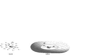
In this paper we will focus on the remaining topological case.
The emitter is seated at the center of a spherical cavity
drilled in a homogeneous medium. This medium is continuous as seen by the
emitter provided that the cavity radius, , is much larger than any correlation length between the
constituents of the host medium, . Thus, the cavity is real. On the other hand, if the wavelength of the emitted field, , is that long that it cannot resolve neither the microscopical structure of the medium nor the cavity, the medium is also continuous as seen by the propagating field. Consequently, the host medium is characterized by a scalar
susceptibility which does not present spatial
dispersion. Topologically, this setup corresponds to that of a
simply-connected-non-contractible manifold with a unique hollow sphere –see Fig.1. Regarding the emitter nature, two scenarios will be addressed for their potential interest in biological imaging and signal processing. In the first one, the emitter will be a polarizable particle excited by an external fixed field of frequency much lower than any of the resonance frequencies of the emitter. The physical quantity to compute in this case will be the power emission, . In the second case, the emitter will be a polarizable particle which decays at some resonance frequency. Dipole induction will be encoded in the emitter itself as it will be assumed to be of Lorentz-type. Thus, the net effect of the host medium will reflect on a variation in the spontaneous decay rate, , together with a shift in the resonance frequency with respect to those values in free space.
In the first scenario, the formula for the power emitted by an induced dipole reads
| (1) | |||||
| (2) | |||||
| (3) |
where is the frequency of the exciting field , with much lower than any internal resonance frequency and is the electrostatic polarizability of the emitter in vacuum, being its dielectric contrast and its radius. For our topological setup, the -factors are given by MeI
| (4) | |||||
| (5) | |||||
with evaluated at and where the cavity factors are
| (6) | |||||
| (7) | |||||
with .
In these equations, is the Fourier transform of the correlation function which describes the isolation of the emitter within a real cavity.
For a spherical cavity of radius , . In the above equations and are respectively the
transverse and longitudinal components of the renormalized propagator
of the coherent –macroscopic– electric field in the host
medium. They read,
,
,
being a unitary vector along the propagation direction
and being the
projective tensor orthogonal to the propagation direction. In
these expressions,
.
Because no spatial dispersion is assumed in the continuous medium,
are functions
of only. are the
components of the propagator of the electric field in free space with bare wave number .
They are given by the above formulae, , , with
.
In the second scenario, the emitter nature differs from that in MeII . In the present case, the dipole moment of the emitter is not a linear combination of a fixed and an induced dipole. Rather than that, the emitter is polarizable in its own and its polarizability function gets renormalized as a
result of iterative self-polarization processes,
| (8) |
In the above equation, the -factors are those in Eqs.(4,5). In addition, the term has been introduced to account for the internal resonance of the emitter in vacuum. As shown in deVriesRMP , it plays the role of a regulator of the intrinsic ultraviolet divergence in . That is, , where is the corresponding real electrostatic polarizability and is the resonance wave number in vacuum. Following deVriesPRL , by parametrizing Eq.(8) in a Lorentzian (L) form, , we can identify the decay rate of the emitter in the host medium as
| (9) | |||||
where is a real non-negative root of the equation
| (10) |
is the renormalized electrostatic polarizability and is the in-vacuum emission rate. As argued in deVriesPRL , consistency with Fermi’s golden
rule requires , being the transition amplitude between
two atomic levels in vacuum.
In view of Eqs.(1,2,3,9), we can address in parallel the computation of and for each
scenario described above. The computation reduces to the evaluation of for and respectively.
Following MeI ; MeII , we will decompose and in
transverse and longitudinal components, and
respectively.
Neglecting longitudinal resonances as in
MeII , only the transverse components contain propagating
modes, and respectively,
which are proportional to the coherent intensity and so to
. It is convenient to
identify their specific contribution to and
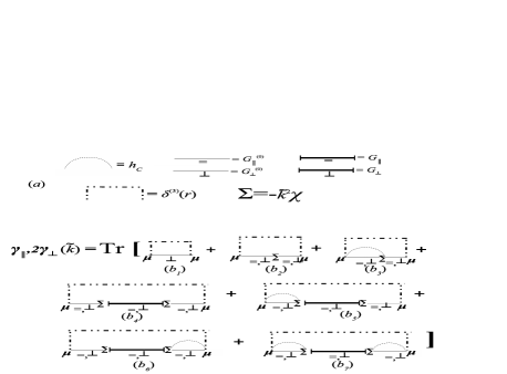
for observational purposes in imaging. Propagating
modes are those associated to complex poles of the propagators in
the integrands of eq.(4). We can read their contribution
from the diagrams in Fig.2,
| (11) |
where the first term on the right hand side (r.h.s) of Eq.(11) contains the contribution of
bulk propagation –transverse components of diagrams (),
(), () in Fig.2.
All the above integrals in Eqs.(4-7,11) can be performed analytically at any order in . However, for the sake of consistency with the approximations considered so far, we take the limit
and keep leading order terms,
| (12) |
It is our choice to normalize to the propagating power in vacuum, . Thus, reads
| (13) | |||||
| (14) | |||||
| (15) |
where is the renormalization factor due to self-polarization cycles. Written this way, we recognize in the first term of the r.h.s of Eq.(13) the usual bulk term corrected by Lorentz-Lorenz (LL) local field factors Lorentz , . The second term there includes corrections of order . It is also remarkable that if the empty-cavity Onsager–Böttcher (OB) Onsager ; GL local field factors are used instead, does agree with the two terms of Eq.(13) up to order . The terms in Eq.(14) are associated to absorbtion in the host medium Loudon ; MeII while that in Eq.(15) corresponds to absorbtion in the emitter. The propagating emission reads
| (16) | |||||
As shown in MeII at leading order, the second term in
Eq.(16) subtracts from the total the
non-propagating, non-absorptive longitudinal contribution.
It is worth comparing this result with that obtained in MeII .
There, provided that follows Maxwell-Garnett (MG) formula vanTiggelen and neglecting absorbtion,
| (17) |
Eq.(16) and Eq.(17) agree at leading order
in . However, in MeII the cermet topology was
considered and the emitter was placed at the site of one of the
host scatterers.
The coincidence of both approaches at leading order bases on the fact that the limit , with being the radius of the exclusion volume between host scatterers, is implicit in Eq.(17). Therefore, no spatial dispersion enters –hence, MG holds– and the radius of the virtual cavity also satisfies as in the present case.
It is straightforward to write in function of
the effective refraction index and the extinction coefficient , with the extinction mean
free path, using the identities
and ,
| (18) | |||||
For the sake of completeness, we give also the values of the non-propagating emission in terms of , and ,
| (19) | |||||
| (21) |
where Eqs.(19,Dipole emission and coherent transport in random media III. Emission from a real cavity in a continuous medium,21) correspond to the power absorbed by the emitter, the transverse non-propagating power, , and the longitudinal emission, , respectively.
Further on, by invoking causality, Kramers-Kronig sum rules relate and
and variations of
can be obtained as a function of LoudonII .
Let us introduce next the self-polarization effect. This is done by multiplying all the expressions above for by the renormalization factor . Neglecting absorbtion both in the emitter and in the host medium, we obtain at leading order in ,
| (22) |
where is the volume of the emitter cavity. In contrast, the OB renormalization factor due to self-polarization reads Onsager ; Bullough ; deVriesPRL ,
| (23) |
Eq.(22) and Eq.(23) differ just in the local field factor which multiplies
in each expression. With this result we finalize the computation of in the first scenario.
In the following, we address the scenario where the emitter is of Lorentzian kind and compute
Eqs.(8-10). We first solve for the renormalized resonance wave vector ,
| (24) | |||||
| (25) |
At leading order in , the first two terms in Eq.(24) equal the expression found in deVriesPRL
for an interstitial emitter. The additional terms in Eq.(25) are relevant for
strongly absorptive media. That may be for instance the case of nano-antennas in metallic media Antenas . Additional solutions to the one above for are only admissible beyond
the small cavity limit and/or the continuous medium approximation. That is, for
and/or , Eq.(10) may contain several real solutions. That
might give rise to a splitting of the in-vacuum resonant peak provided such an splitting is broader than
the line width. The origin of the resonance shifts of Eqs.(24,25) is in the virtual photons
which dress up the polarizability through Eq.(8). Those photons trace closed
spatial loops as depicted by the diagrams in Fig.(2). They amount to a classical continuum of
sates not to be confused with real localized photons. The resultant frequency shift must be rather
interpreted as the classical analog to the quantum Lamb shift Wylie ; Sakurai . On the other hand, the possibility of a
resonance splitting would be subjected to
consistency with our perturbative renormalization scheme and linear-response approximation.
Finally, we give the full expression for at lowest order in according to Eq.(9),
| (26) | |||||
Eqs.(24-26) can be compared with the results of deVriesPRL ; Fleisch .
In summary, following MeI , we have found analytical
expressions for the power emitted by an induced dipole
–Eqs.(13,14,15,22)–
and for the spontaneous emission rate of a
Lorentzian-type emitter –Eqs.(9,26)– from
a real cavity in a continuous medium. In the former case we
compute both the propagating and non-propagating power emission
–Eq.(18) and Eqs.(19-Dipole emission and coherent transport in random media III. Emission from a real cavity in a continuous medium) respectively– in
function of the complex index of refraction. In the latter case,
we also compute the shift in the resonance frequency
–Eqs.(10,24,25).
We found that, in the small cavity limit, , the tuning of may be sensitively affected
by a strongly absorptive metallic environment –Eq.(25). Beyond that limit and/or the continuous medium
approximation, we argue on the possibility of obtaining additional resonance frequencies.
This work has been supported by Microseres-CM and the EU
Integrated Project ”Molecular Imaging” (LSHG-CT-2003-503259).
References
- (1) E.M. Purcell, Phys. Rev. 69, 681 (1946).
- (2) K. Suhling, P.M. W. French and D. Phillips, Photochem. Photobiol. Sci. 4, 13 (2005).
- (3) V.V. Protasencko, A.C. Gallagher, Nano. Lett. 4, 1329 (2004); J.N. Farahani, D.W. Pohl, H.J. Eisler and B. Hecht, Phys. Rev. Lett. 95, 017402 (2005); R. Carminati, J.J. Greffet, C. Henkel and J.M. Vigoureux, Opt. Com. 261 (368).
- (4) E. Yablonovitch, Phys. Rev. Lett. 58, 2059 (1987); S. John, Phys. Rev. Lett. 58, 2486 (1987); S. John and T. Quang, Phys. Rev. A 50, 1764 (1994).
- (5) M. Donaire and J.J. Saenz, e-print arXiv:0811.0323.
- (6) M. Donaire, e-print arXiv:0811.0373.
- (7) P. de Vries, D,V. van Coevorden and A. Lagendijk, Rev. Mod. Phys. 70, 447 (1998).
- (8) P. de Vries and A. Lagendijk, Phys. Rev. Lett. 81, 1381 (1998).
- (9) A. Lagendijk et al. Phys. Rev. Lett. 79, 657 (1997).
- (10) H.A. Lorentz, Wiedem. Ann. 9, 641 (1880); L. Lorenz, Wiedem. Ann. 11, 70 (1881).
- (11) S.M. Barnett, B. Huttner and R. Loudon, Phys. Rev. Lett. 68, 3698 (1992); S.M. Barnett, B. Huttner, R. Loudon and R. Matloob, J. Phys. B 29, 3763 (1996); L.S. Froufe-Perez, R. Carminati and J.J. Saenz, Phys. Rev. A 76, 013835 (2007).
- (12) S.M. Barnett and R. Loudon, Phys. Rev. Lett. 77, 2444 (1996); R. Carminati and J.J. Saenz, to appear in Phys. Rev. Lett. (2009).
- (13) F. Hynne and R.K. Bullough J. Phys. A 5, 1272 (1972); F. Hynne and R.K. Bullough, Phil. Trans. R. Soc. Lond. A 321, 305 (1987).
- (14) L. Onsager, J. Am. Chem. Soc. 58, 1486 (1936); C.J.F.Böttcher, Theory of Electric Polarization Elsevier, Amsterdam (1973)
- (15) J.M. Wylie and J.E. Sipe, Phys. Rev. A 30, 1185 (1984).
- (16) J.J. Sakurai, Advanced Quantum Mechanics Additon-Wesley (1973).
- (17) R. Glauber and M. Lewenstein , Phys. Rev. A 43, 467 (1991).
- (18) M.Fleischhauer, Phys. Rev. A 60, 2534 (1999).