On the Dynamics of the Error Floor Behavior
in (Regular) LDPC Codes

Abstract

It is shown that dominant trapping sets of regular LDPC codes, so called absorption sets, undergo a two-phased dynamic behavior in the iterative message-passing decoding algorithm. Using a linear dynamic model for the iteration behavior of these sets, it is shown that they undergo an initial geometric growth phase which stabilizes in a final bit-flipping behavior where the algorithm reaches a fixed point. This analysis is shown to lead to very accurate numerical calculations of the error floor bit error rates down to error rates that are inaccessible by simulation. The topology of the dominant absorption sets of an example code, the IEEE 802.3an $(2048,1723)$ regular LDPC code, are identified and tabulated using topological relationships in combination with search algorithms.

I Summary

The error floor in modern graph-based error control codes such as low-density parity-check codes is caused by inherent structural weaknesses in the code’s interconnect network. The iterative message passing algorithm cannot overcome these weaknesses and gets trapped in error patterns which are easily identifiable as erroneous (in LDPC codes), and are thus not valid codewords, but difficult to overcome or correct [1, 2]. These weaknesses were termed trapping sets by Richardson in [3], a summary definition for the patterns on which the message passing algorithm fails for Gaussian channels. These trapping sets are dependent on the code, the channel used, and to a lesser degree also on the details of the decoding algorithm. Prior work in identifying the weaknesses of LDPC codes on erasure channels led to the definition of stopping sets in [4]. Stopping sets, being the weaknesses of LDPC codes on erasure channels, also play a role on Gaussian channels, but are not typically the dominant error mechanisms. In [5] the authors define absorption sets, which are the subgraphs of the code graph on which the Gallager bit-flipping decoding algorithms fail for binary symmetric channels. The authors observed that these absorption sets also show up as the dominant trapping sets in certain structured LDPC codes. In [6] they devise post-processing methods to reduce the effects of these absorption sets and lower the error floor of the codes in question.

In this paper we present a linear algebraic approach to the dynamic behavior of absorption sets. We show that these sets follow a geometric growth phase during early iterations where messages inside the absorption set grow towards a largest eigenvector which characterizes the absorption set. The seemingly erratic behavior of the messages at early iterations is due to the decreasing influence of lesser eigenvectors. We define the gain of an absorption set and show how it affects the influence of the extrinsic messages that flow into the absorption set at each iteration from the remainder of the code network. The importance of set extrinsic information was already informally observed in [7], who reported a lowering of the error floor with increased extrinsic connectivity. We use our analysis to produce accurate error formulas for the error floor BER/FER and support these results with importance sampling simulations targeting the absorption sets.

As illustration we carefully identify and classify absorption sets of the regular $(2048,1723)$ LDPC code recently designed in [8], which is used in the IEEE 802.3an standard.

Topological features of dominant absorption sets are identified and a search algorithm is presented which finds the leading dominant sets.

II Background

Stopping sets completely determine the performance of graph-based decoding of LDPC codes on erasure channels, i.e., on channels where the transmitted binary symbols are either received correctly, or are erased. A complete statistical treatment of stopping sets was given in [4]. Aptly named, a stopping set is a subset of uncorrected variable nodes where the decoder stops, i.e., makes no further correction progress. It is simply defined as:

Definition 1.

A stopping set $\cal S$ is a set of variable nodes, all of whose neighboring check nodes are connected to the set $\cal S$ at least twice.

Figure1 shows an example of a stopping set. It is quite straightforward to see that if erasure decoding is performed following Gallager’s decoding algorithm [9] the variable values in the stopping set cannot be reconstructed. Valid codewords are trivially stopping sets, but the set of stopping sets is larger than the set of valid codewords.

Figure 1: Example of a stopping set.

An absorption set is an extension of the notion of a stopping set to the binary-symmetric channels [5, 6], and is defined as:

Definition 2.

An absorption set $\cal A$ is a set of variable nodes, such that the majority of each variable node’s neighbors are connected to the set $\cal A$ an even number of times.

Figure2 shows an example absorption set. It can be verified that Gallager-type bit flipping decoding will not be able to correct an absorption set, since a majority of messages impinging on each variable node will retain the erroneous sign for each iteration. Consequently, the algorithm locks up.

Figure 2: Example of an absorption set.

III LDPC Codes on the Gaussian Channel

The Gaussian channel is different from the binary symmetric and binary erasure channels and causes a more complicated error behavior on LDPCs. Richardson [3] first seriously explored the error floor of LDPCs on Gaussian channels and defined trapping sets as the failure mechanism. Noting that typically very few trapping sets dominate the error floor region he proposed a semi-analytical method which amounts to a variant of importance sampling to numerically predict the error floor from the knowledge of a code’s trapping sets.

While finding trapping sets remained a largely open problem, [5] observed that in certain structured LDPCs the dominant trapping sets are absorption sets, i.e., the failure mechanism of the code on binary symmetric channels. In [6], algorithmic modifications were proposed to “eliminate” the error floor caused by these absorption sets.

Due to its popularity and extensive exposure we will concentrate on the $(2048,1723)$ regular LDPC code [8] used in the IEEE 802.3an standard. This code has been extensively analyzed. It has a low error floor that appears at $E_{b}/N_{0}\approx 5$dB at a BER of $10^{-12}$, that is too low to be efficiently explored using conventional simulations.

Figure3 shows the structure of the dominant absorption set of this code (see also [6, Figure2]). There are $14,272$ such sets in the $(2048,1723)$ code of [8]. They dominate the error floor since they are the minimal absorption sets in this code (for definition of minimal and dominant, see Definition 4).

Figure 3: A dominant absorption set of the IEEE 802.3an code (not all check node connections shown).

III-A Finding Dominant Absorption Sets

The $(2048,1723)$ rate $0.8413$ regular LDPC code [8] considered here has a structured parity-check matrix:

$$\mathbf{H}=\begin{bmatrix}\mathbf{\sigma}_{11}&\mathbf{\sigma}_{12}&\mathbf{\sigma}_{13}&\cdots&\mathbf{\sigma}_{1,32}\\ \mathbf{\sigma}_{21}&\mathbf{\sigma}_{22}&\mathbf{\sigma}_{23}&\cdots&\mathbf{\sigma}_{2,32}\\ \mathbf{\sigma}_{31}&\mathbf{\sigma}_{32}&\mathbf{\sigma}_{33}&\cdots&\mathbf{\sigma}_{3,32}\\ \vdots&\vdots&\vdots&\ddots&\vdots\\ \mathbf{\sigma}_{61}&\mathbf{\sigma}_{62}&\mathbf{\sigma}_{63}&\cdots&\mathbf{\sigma}_{6,32}\\ \end{bmatrix}_{384\times 2048}$$

where each $\mathbf{\sigma}_{ij}$ is a $64\times 64$ permutation matrix.

Definition 3.

Let $(a,b)$ denote an absorption set, where $a$ is the size of the set (number of variable nodes) and $b$ is the extrinsic message degree (EMD), i.e., the cardinality of the set of the neighboring check nodes that are connected to the set an odd number of times (the unsatisfied checks).

For example, Figure2 and Figure3 show $(4,4)$ and $(8,8)$ absorption sets, respectively.

Table I shows the first few absorption sets of the code in [8].

TABLE I: Absorption sets of IEEE 802.3an LDPC code.

$a$	$b$	Existence	Multiplicity	Gain
$<5$		No
$5$	$10$	No
$6$	$6$	No
	$8$
	$10$
	$12$
$7$	$0$	No
	$2$
	$4$
	$6$
	$8$
	$10$
	$12$	Yes	$65,472$	$3.29$
	$14$	Yes	?	$3$
$8$	$0$	No
	$2$
	$4$
	$6$
	$8$	Yes	$14,272$	$4$
	$10$	No
	$12$	Yes	$44,416$	$3.5$
	$14$	Yes	?	$3.25$
	$16$			$3$
$9$	$0$	No
	$2$
	$4\leq b\leq 10$	?
	$12$	Yes	?	$3.67$
	$14$			$3.44$
	$16$			$3.22$
	$18$			$3$
$10$	$\leq 8$	?
	$10$	Yes	$>192$	$4$
	$12$	Yes	?	$3.8$
	$14$			$3.6$
	$16$			$3.4$
	$18$			$3.2$
	$20$			$3$

Definition 4.

(i) Let the ratio $b/a$ denote the average EMD for an $(a,b)$ absorption set. (ii) An $(a,b)$ absorption set is called minimal if no $(a^{\prime},b^{\prime})$ absorption set exists with $a^{\prime}<a$ and $b^{\prime}/a^{\prime}\leq b/a$, i.e., less variable nodes and smaller average EMD. (iii) A minimal $(a,b)$ absorption set is called dominant if no $(a,b^{\prime})$ absorption set exists with $b^{\prime}<b$, i.e., smaller EMD.

The smaller the absorption set, the more severe the effect on the error floor. Thus our target is to find the dominant absorption sets in terms of $a$, $b$ and $b/a$. Since the variable node degree $d_{v}=6$, $a\geq 5$ by the definition of absorption sets and the code is $4$-cycle free. In addition, $b\in[0,2a]$ and must be even. So let us start with $a=5$ to develop the numbers in Table I. The coefficient $5-b/a$ is the gain of the absorption set, which determines how fast the extrinsic information enters the set — see later.

III-A1 $a=5$

Clearly $b$ can only equal $10$ and there is only one possible connecting topology shown in Figure4.

(a) Check nodes shown.

(b) Check nodes hidden.

Figure 4: The only possible topology of $(5,10)$ absorption sets.

Lemma 1.

There are no size-$5$ absorption sets.

Proof:

See Appendix A. ∎

III-A2 $a=6$

Let us introduce additional notations needed to prove the existence of absorption sets.

Definition 5.

(i) For any variable node $v$ in an absorption set, let $\mathrm{Deg}(v)$ denote the number of neighboring check nodes of $v$ that are connected to the set an even number of times. $\mathrm{Deg}(v)$ is the degree of vertex $v$ in the topology graph with check nodes hidden. (ii) Let an unordered array $[\mathrm{Deg}(v_{i}):i=1,2,\ldots,a]$ denote a class of $(a,b)$ absorption sets, where $\mathrm{Deg}(v_{i})\in\{4,5,6\}$ and $\sum\limits_{i=1}^{a}\mathrm{Deg}(v_{i})=6a-b$.

It is difficult to find absorption sets, even by making use of Algorithm 1-type methods (see Appendix A), due to their extremely low appearance. Hence we need Definition 5 to classify the absorption sets first. For each pair $(a,b)$, there may be several classes of absorption sets, and each class may exhibit several topologies. What we are trying to do is to reduce one unknown absorption set to a smaller absorption set whose non-existence is known by eliminating nodes from the original set. We can then argue that there is only a limited number of topologies that have to be searched algorithmically.

Theorem 2.

There are no size-$6$ absorption sets.

Proof:

See Appendix B. ∎

III-A3 $a=7$

Theorem 3.

There are no $(7,b)$ absorption sets with $b<12$. $(7,12)$ and $(7,14)$ absorption sets do exist.

Proof:

See Appendix C. ∎

III-A4 $a=8$

First we show

Lemma 4.

For $b<8$, there exist no $(8,b)$ absorption sets. For $b=8$, there exists no $(8,8)$ absorption set that contains a degree-$6$ variable node.

Proof:

See Appendix D. ∎

Then the only possible class of $(8,8)$ absorption set would have connectivity $[5,5,5,5,5,5,5,5]$. We claim that

Claim 1.

Graphically, there exist five possible topologies for $[5,5,5,5,5,5,5,5]$ absorption sets, shown in Figure17, 18 and 22.

Proof:

See Appendix E. ∎

Theorem 5.

The number of $(8,8)$ absorption sets is $14,272$ and they all have the topology of Figure22.

Proof:

By searching all topologies in Claim 1 on the $\mathbf{H}$ matrix of [8]. ∎

Since these are the dominant absorption sets, let us sketch their connections in Figure5 one more time.

Figure 5: $(8,8)$ absorptions sets.

The average multiplicity of each variable node appeared in such sets is $14272\times 8/2048=55.75$. Because of the block structure of the $\mathbf{H}$ matrix, certain groups of variable nodes do share the same multiplicity, as listed in Table II. The ratio $b/a=1$. The next possible absorption set with these parameters would be the $(10,10)$ set.

TABLE II: The multiplicity of each variable node in $(8,8)$ absorption sets.

Variable Nodes	Multiplicities	Variable Nodes	Multiplicities
$0$—$63$	$63$	$1024$—$1087$	$54$
$64$—$127$	$55$	$1088$—$1151$	$66$
$128$—$191$	$74$	$1152$—$1215$	$49$
$192$—$255$	$60$	$1216$—$1279$	$40$
$256$—$319$	$67$	$1280$—$1343$	$75$
$320$—$383$	$68$	$1344$—$1407$	$41$
$384$—$447$	$54$	$1408$—$1471$	$56$
$448$—$511$	$60$	$1472$—$1535$	$59$
$512$—$575$	$57$	$1536$—$1599$	$47$
$576$—$639$	$66$	$1600$—$1663$	$36$
$640$—$703$	$60$	$1664$—$1727$	$59$
$704$—$767$	$49$	$1728$—$1791$	$59$
$768$—$831$	$39$	$1792$—$1855$	$37$
$832$—$895$	$47$	$1856$—$1919$	$52$
$896$—$959$	$61$	$1920$—$1983$	$69$
$960$—$1023$	$62$	$1984$—$2047$	$43$

III-B Less Dominant Absorption Sets

There exist larger and less dominant absorption sets. See Appendix F for details.

IV Dynamic Analysis of Absorption Sets

We now present a linearized analysis to gain insight into the behavior of dominant absorption sets starting with the leading $(8,8)$ absorption set. First we note that the variable nodes perform simple addition. Furthermore, the check nodes basically choose the minimum of the incoming signals. If we make the reasonable assumption that the absorption set converges slower than the remaining nodes in the code, and due to the fact that each (satisfied) check node is connected exactly to two absorption set variables, the minimum absolute-value signal into the participating check nodes will come from one of the absorption set variables. If this is true, the check nodes simple exchange the signals on the connections to the absorption set variable nodes. We will refine this approximation below.

Additionally, each absorption set variable node is singly connected to a “lone” floating extrinsic parity check node, all of whose other connections go to other, set-external variable nodes. The messages through these eight extrinsic check nodes are the extrinsic messages into the absorption set, and are of crucial importance. Algorithmically, they play exactly the same role as the intrinsic channel values which are fed into the variable nodes by virtue of the summation function executed at the variable nodes.

Figure6 shows an example of the dynamic behavior of the absorption set variables close to its decision threshold boundary. The seemingly erratic behavior resolves after a number of iterations when all variables follow highly correlated trajectories. This observation is the basis for the following analysis.

Figure 6: Dynamics of an absorption set close to the decision boundary. The different curves are the variable node LLR values for the eight absorption set nodes.

$$P_{\rm AS}=Q\left(\frac{\displaystyle 2m_{\lambda}+2\sum\limits_{j=1}^{I}\left(\frac{m_{\lambda^{(ex)}}^{(j)}+m_{\lambda}}{\mu_{\rm max}^{j}}\prod\limits_{l=1}^{j}\frac{1}{g_{l}}\right)}{\sqrt{\displaystyle\left(1+\sum_{j=1}^{I}\prod_{l=1}^{j}\frac{1}{g_{l}\mu_{\rm max}}\right)^{2}m_{\lambda}+\sum_{j=1}^{I}m_{\lambda^{(ex)}}^{(j)}\left(\prod_{l=1}^{j}\frac{1}{g_{l}\mu_{\rm max}}\right)^{2}}}\right)$$ (7)

Denote the outgoing solid edge values from the variable nodes (Figure3) by $x_{i}$, i.e., $x_{1},\cdots,x_{5}$ leave variable node $v=0$, $x_{6},\cdots,x_{10}$ variable node $v=1$, etc. Collect the $x_{i}$ in the length-$40$ column vector $\mathbf{x}$, which is the vector of outgoing variable edge values in the absorption set. Likewise, and analogously, let $\mathbf{y}$ be the incoming edge values to the variable nodes, such that $y_{j}$ corresponds to the reverse-direction message. Now, at iteration $i=0$

$$\mathbf{x}_{0}=\boldsymbol{\lambda}$$

where the initial input is the vector of channel intrinsics $\boldsymbol{\lambda}=\left[\lambda_{1},\cdots,\lambda_{1},\lambda_{2},\cdots,\lambda_{2},\cdots,\lambda_{8},\cdots,\lambda_{8}\right]^{\mathrm{T}}$ duplicated onto the outgoing messages. It undergoes the following operation at the check node:

$$\mathbf{y}_{0}=\mathbf{Cx}$$

where $\mathbf{C}$ is a permutation matrix that exchanges the absorption set signals as discussed above. At iteration $i=1$ we obtain

$$\mathbf{x}_{1}=\mathbf{VC}\boldsymbol{\lambda}+\boldsymbol{\lambda}+\boldsymbol{\lambda}_{1}^{(ex)}$$

where $\mathbf{V}$ is the variable node function matrix, i.e., each output is the sum of the other four inputs from the check nodes plus the intrinsic input. The extrinsic inputs from the remainder of the code graph are contained in $\boldsymbol{\lambda}_{1}^{(ex)}$. Following the linear model, at iteration $I=j$ extrinsic signals are injected into the absorption set as $\boldsymbol{\lambda}^{(ex)}_{j}=\left[\lambda^{(ex)}_{j1},\cdots,\lambda^{(ex)}_{j1},\lambda^{(ex)}_{j2},\cdots,\lambda^{(ex)}_{j8}\right]^{\mathrm{T}}$ via the extrinsic check nodes. By induction we obtain at iteration $i=I$

$$\mathbf{x}_{I}=\sum_{i=0}^{I}(\mathbf{VC})^{i}\boldsymbol{\lambda}+\sum_{j=1}^{I}\sum_{i=j}^{I}(\mathbf{VC})^{i}\boldsymbol{\lambda}_{j}^{(ex)}$$

Applying the spectral theorem we obtain

$$(\mathbf{VC})^{i}\mathbf{\lambda}\rightarrow\mu_{\rm max}^{i}\left(\mathbf{\lambda}^{\mathrm{T}}\mathbf{v}_{\rm max}\right)\mathbf{v}_{\rm max}$$

where $\mathbf{v}_{\rm max}$ is the unit-length eigenvector of the maximal eigenvalue $\mu_{\rm max}$ of the matrix $\mathbf{VC}$.

The following lemma holds:

Lemma 6.

The largest eigenvalue of $\mathbf{VC}$ for the $(8,8)$ set is $\mu_{\rm max}=d_{v}-2=4$, and its associated eigenvector is $\mathbf{v}_{\rm max}=[1,\cdots,1]^{\mathrm{T}}$.

Proof:

First write $\mathbf{VC}=4\mathbf{M}$. By inspection $\mathbf{M}$ is a probability matrix, i.e., the sum of all rows equals unity. As a special case of the Perron-Frobenius theorem it is known that the largest eigenvalue of a probability matrix is $1$, therefore the largest eigenvalue of $\mathbf{VC}$ equals $4$. By inspection $\mathbf{VC}[1,\cdots,1]^{\mathrm{T}}=4[1,\cdots,1]^{\mathrm{T}}$. ∎

The absorption set in question falls in error if

$$\beta=\boldsymbol{\lambda}^{\mathrm{T}}\mathbf{v}_{\rm max}+\sum_{j=1}^{I}\frac{\left({\boldsymbol{\lambda}_{j}^{(ex)}}+\boldsymbol{\lambda}\right)^{\mathrm{T}}\mathbf{v}_{\rm max}}{\mu_{\rm max}^{j}}\leq 0$$ (1)

or, in the case of the $(8,8)$ absorption set

$$\beta=\sum_{i=1}^{8}\left(\lambda_{i}+\sum_{j=1}^{I}\frac{\lambda^{(ex)}_{ji}+\lambda_{i}}{\mu_{\rm max}^{j}}\right)\leq 0$$ (2)

The eigenvalue $\mu_{\rm max}=d_{v}-2$ is the gain of the absorption set and it is determined by the variable node degree.

Exact knowledge of $\lambda^{(ex)}_{ji}$ is not available to the analysis, since these values depend on the received signals. However, assuming that the code structure extrinsic to the apsorption set operates “regularly”, we may substitute average values for the $\lambda^{(ex)}_{ji}$. Note that $\lambda_{i}$ is Gaussian distributed from the channel, and that we may assume that $\lambda^{(ex)}_{ji}$ is also Gaussian distributed as is customary in density evolution analysis [10, 9]. Furthermore, like $\lambda_{i}$, we assume that $\lambda^{(ex)}_{ji}$ has a consistent Gaussian distribution with $m=2\sigma^{2}$, where $m$ is the mean. We therefore only need the mean of $\lambda^{(ex)}_{ji}$, which we can calculate from a Gaussian density evolution calculation, i.e.,

$$m_{\lambda^{(ex)}}^{(i)}=\phi^{-1}\left(1-\left[1-\phi\left(m_{\lambda}+(d_{v}-1)m_{\lambda^{(ex)}}^{(i-1)}\right)\right]^{d_{c}-1}\right)$$

where $m_{\lambda}=2E_{b}/\sigma^{2}$ is the mean of $\lambda_{i}$, $m_{\lambda^{(ex)}}^{(i)}$ is the mean of the extrinsic signal $\lambda^{(ex)}_{ji}$, and $\phi$ is the check node mean transfer function [9].

With the Gaussian assumptions, the probability of (2) happening can be calculated as

$$P_{\rm AS} {}={} {\rm Pr}\left(\beta\leq 0\right)$$ (3)

$$= Q\left(\frac{\displaystyle 2m_{\lambda}+2\sum\limits_{j=1}^{I}\frac{m_{\lambda^{(ex)}}^{(j)}+m_{\lambda}}{\mu_{\rm max}^{j}}}{\sqrt{\displaystyle\left(1+\sum_{j=1}^{I}\frac{1}{\mu_{\rm max}^{j}}\right)^{2}m_{\lambda}+\sum_{j=1}^{I}\frac{m_{\lambda^{(ex)}}^{(j)}}{\mu_{\rm max}^{2j}}}}\right)$$

Two refinements can be added to this analysis. The exchange of extrinsics through the matrix $\mathbf{C}$ is an approximation in two ways: (i) As long as the remaining $d_{c}-2=30$ inputs to the check node are relatively small, the entries of $\mathbf{C}$ are strictly less than unity, and, (ii) in case one of the extrinsic incoming check node messages has the wrong polarity, the returned signal to the absorption set switches polarity. Case (i) is approached as follows. Using a Taylor series approximation we show that the quintessential check node operation

$$\tanh^{-1}\left(\tanh(x)\prod_{i=1}^{d_{c}-2}\tanh(x_{i})\right)=\prod_{i=1}^{d_{c}-2}\tanh(x_{i})\,x+O\left[x^{3}\right]$$

where $\prod\limits_{i=1}^{d_{c}-2}\tanh(x_{i})$ can be interpreted as a “check node gain”. If we use for $x_{i}$ the mean $m_{\mu^{(ex)}}^{(i)}$ of the signals $\mu^{(ex)}$ from the variable to the check nodes, an average gain can be computed as

$$g_{i} {}={} E\left[\prod_{i=1}^{d_{c}-2}\tanh\left(\frac{m_{\mu^{(ex)}}^{(i)}}{2}\right)\right]$$ (4)

$$= E\left[\tanh\left(\frac{m_{\mu^{(ex)}}^{(i)}}{2}\right)\right]^{d_{c}-2}$$ (5)

$$= \left(1-\phi\left(m_{\mu^{(ex)}}^{(i)}\right)\right)^{d_{c}-2}$$ (6)

where the last equality results from the definition of the density evolution function $\phi(\cdot)$. With this result the probability in (3) is modified to (7). In the case of general sets we need to work with (1) instead, and compute $\mu_{\rm max}$ and $\mathbf{v}_{\rm max}$ numerically using the set topology.

$$f(a,b)=\frac{\displaystyle am_{\lambda}\left(1+\sum_{j=1}^{I}\prod_{l=1}^{j}\frac{1}{g_{l}\left(5-\frac{b}{a}\right)^{j}}\right)+b\sum\limits_{j=1}^{I}\left(\frac{m_{\lambda^{(ex)}}^{(j)}}{\left(5-\frac{b}{a}\right)^{j}}\prod\limits_{l=1}^{j}\frac{1}{g_{l}}\right)}{\displaystyle\sqrt{\displaystyle 2am_{\lambda}\left(1+\sum_{j=1}^{I}\prod_{l=1}^{j}\frac{1}{g_{l}\left(5-\frac{b}{a}\right)}\right)^{2}+2b\sum_{j=1}^{I}m_{\lambda^{(ex)}}^{(j)}\left(\prod_{l=1}^{j}\frac{1}{g_{l}\left(5-\frac{b}{a}\right)}\right)^{2}}}$$ (11)

Case (ii) can be handled by the linear analysis as well in the following way. If an external variable to the absorption set has an incorrect sign, this reverses the polarity of the signal returned to the absorption set from that particular check node. During the first iteration, these extrinsic signals are basically the received channel LLRs from the connected variable nodes. The probability that these are in error is given by the raw bit error rate

$$P_{e}=Q\left(\sqrt{2\frac{E_{s}}{N_{0}}}\right)$$ (8)

There are $d_{c}-2=30$ external inputs impinging on each check node of the absorption set, therefore the probability that a returned signal experiences a polarity reversal is given by

$$P_{p}=\sum_{k=1}^{14}{30\choose 2k+1}P_{e}^{2k+1}\left(1-P_{e}\right)^{29-2k}$$ (9)

The model in (7) can now be expanded by injecting a correction value into the absorption set node whenever an external value is in error. We assume that if a polarity reversal occurs, the minimum value of the check node is likely close to zero, therefore the injected correction value needs to cancel the absent feedback signal and is set to $-\lambda_{{\rm ex},i}/\mu_{\rm max}$. If $k$ check nodes are in error, $2k$ correction values are injected, one for each message going back to the absorption set. The injected correction values will alter the mean value of the decision variable to

$${\rm mean}\rightarrow 8\left(m_{\lambda}\left(1-\frac{k}{4\mu_{\rm max}}\right)+\sum_{j=1}^{I}\left(\frac{m_{\lambda^{(ex)}}^{(j)}}{\mu_{\rm max}^{j}}\prod_{l=1}^{j}\frac{1}{g_{l}}\right)\right)$$

and the variance is adjusted accordingly, where care needs to be taken how the correction values accumulate. We have used an upper bound on the variance.

Note that these modifications only include check node polarity reversal at the first iteration, but an extension to subsequent iterations is straight-forward if messy. Furthermore, as seen in Figure8 (dashed curves), the addition of this mechanism has only a minor effect on the results.

The probability $P_{\rm AS}$ needs to be multiplied with the multiplicity factor of $14,272$ in order to obtain a union bound. In order to compute a BER estimate, we further multiply this number by $8/1723$, since there are eight errors that occur in a frame of $1,723$ bit errors due to this absorption set.

Figure7 shows $P_{\rm AS}$ for the first most dominant absorption sets. Also shown are general tendencies of $P_{\rm AS}$ as a function of $a$ and $b$:

$$P_{\rm AS}=Q\left(f(a,b)\right)$$ (10)

where $f(a,b)$ is defined by (11). It can be shown that $\mu_{\rm max}\approx 5-b/a$ is a close approximation (exact for symmetric sets with $a=b$) to the gain of the set, and this was used in Figure7 to plot the curves.

It can be seen that the $(8,8)$ absorption set is the most dominant, which is consistent with numerical observations. Multiplicities also affect a set’s impact — see Figure8. Additionally, some sets, like the majority of $(7,12)$ sets, are “contained” in larger sets, that is, such $(7,12)$ absorption sets are not stable under bit flipping and will evolve into $(8,8)$ sets, of which they are subgraphs.

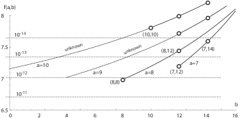
Figure 7: Error probability of dominant absorption sets at $E_{b}/N_{0}=5$dB and approximation functions based on $a$ and $b$. (Curves are drawn only for possible or existing parameter combinations.)

V Numerical Verification

Figure8 shows the analytical error floor calculation using (7) and the multiplicity of $14,272$. Lesser absorption sets have an impact more than an order of magnitude lower. And they are not considered. The figure also shows hardware simulations using an FPGA platform, as well as importance sampled simulations using the same absorption sets as bias targets. Regular mean-shift importance sampling was utilized and each of the absorption sets containing a specific variable node was biased separately. As evidenced by the figure, our linearized analysis provides an accurate picture of the error floor behavior of this code and illustrates the dominance of the $(8,8)$ absorption sets.

Figure 8: IS simulations, FPGA hardware simulations, and analytical error floor analysis for the $(2048,1723)$ regular $(6,32)$ LDPC code.

VI Conclusion

We have presented an analytical analysis of the dynamic behavior of the dominant absorption sets in LDPC message-passing decoders. These absorption sets cause the infamous error floor at high signal-to-noise ratios, and we have identified the dominant such sets for the example regular LDPC code used in the IEEE 802.3an standard via topological arguments and searches. Using importance sampling with the dominant sets accurately predicts the error floor of this code.

Appendix A Proof of Lemma 1

Matrix $\mathbf{H}$ is searched observing the constraints imposed by the absorption set topology. In addition, some of the properties listed in [11, 12] for array-based LDPC codes apply, as well. The following algorithm is used:

Input: Parity-check matrix $\mathbf{H}_{384\times 2048}$ and Figure4.

Output: Absorption sets.

foreach variable node $v\in\{0,1,2,\ldots,2047\}$ do  Pick $4$ out of $6$ neighboring check nodes of $v$ denoted $c_{0},c_{1},c_{2}$ and $c_{3}$, respectively;

foreach one out of $31$ neighboring variable nodes other than $v$ of $c_{0}$, denoted as $v_{1}$ do  foreach one out of $31$ neighboring variable nodes other than $v$ of $c_{1}$, denoted as $v_{2}$ do  if $v_{2}$ and $v_{1}$ are not connected then  re-pick $v_{2}$;

else  foreach one out of $31$ neighboring variable nodes other than $v$ of $c_{2}$, denoted as $v_{3}$ do  if $v_{3}$ and $v_{1}$ or $v_{3}$ and $v_{2}$ are not connected then  re-pick $v_{3}$;

else  foreach one out of $31$ neighboring variable nodes other than $v$ of $c_{3}$, denoted as $v_{4}$ do  if $v_{4}$ and $v_{1}$ or $v_{4}$ and $v_{2}$ or $v_{4}$ and $v_{3}$ are not connected then  re-pick $v_{4}$;

else  follow Definition 2 to determine if this candidate set is an absorption set;

               

Algorithm 1 Algorithm for finding $(5,10)$ absorption sets.

Appendix B Proof of Theorem 2

For $a=6$, there are four possible values for $b$ and there is only one possible topology corresponding to each of them, shown in Figure9.

(a) $(6,6)$

(b) $(6,8)$

(c) $(6,10)$

(d) $(6,12)$

Figure 9: Possible topologies of size-$6$ absorption sets.

By removing any node in Figure9(a) or either degree-$4$ node in Figure9(b), we obtain the $[4,4,4,4,4]$ set, one shown in Figure4(b). By Lemma 1, Figure9(a)–9(b) do not exist. After eliminating topologies Figure9(c)–9(d) algorithmically, Theorem 2 follows.

Appendix C Proof of Theorem 3

Now $a$ is large enough for the neighboring check nodes to be connected to the absorption set four times. First, we suppose that all satisfied check nodes are connected to the set twice.

C-A $b=0$

If $b=0$, then the absorption set is a codeword. However, since $d_{\rm min}\geq 8$ [8], $b\not=0$.

C-B $0<b<12$

We apply the constraints in Definition 5 and the pigeonhole principle to prove this.

1. $b=2$, there are two classes:

   1. $[6,6,6,6,6,5,5]$: removing either degree-$5$ node leaves a $(6,6)$ absorption set.

   2. $[6,6,6,6,6,6,4]$: removing the degree-$4$ node generates a $(6,4)$ absorption set.

2. $b=4$, there are three classes:

   1. $[6,6,6,5,5,5,5]$: removing any degree-$5$ node generates a $(6,8)$ absorption set.

   2. $[6,6,6,6,5,5,4]$: removing the degree-$4$ node generates a $(6,6)$ absorption set.

   3. $[6,6,6,6,6,4,4]$: this is infeasible since the group of five degree-$6$ nodes requires ten edges emanating from the group of degree-$4$ nodes.

3. $b=6$, there are four classes:

   1. $[6,5,5,5,5,5,5]$: removing any degree-$5$ node generates a $(6,10)$ absorption set.

   2. $[6,6,5,5,5,5,4]$: removing the degree-$4$ node generates a $(6,8)$ absorption set.

   3. $[6,6,6,5,5,4,4]$: each of the degree-$5$ nodes and each of the degree-$6$ nodes needs at least one and two edges emanating from the two degree-$4$ nodes, respectively. That makes eight. So there is no connection between the degree-$4$ nodes. Thus removing either of them generates a $(6,8)$ absorption set.

   4. $[6,6,6,6,4,4,4]$: each of the degree-$6$ nodes needs three edges emanating from the two degree-$4$ nodes. That makes twelve. So there is no connection among the three degree-$4$ nodes. Thus removing any of them generates a $(6,8)$ absorption set.

4. $b=8$, there are four classes:

   1. $[5,5,5,5,5,5,4]$: removing the degree-$4$ node generates a $(6,10)$ absorption set.

   2. $[6,5,5,5,5,4,4]$: let us study the intrinsic connections between the two degree-$4$ nodes:

      Figure 10: Possible intrinsic connections between two degree-$4$ nodes.

      1. Not connected as shown in Figure10: removing either degree-$4$ node will reduce it to a $(6,10)$ absorption set.

      2. Connected as shown in Figure10: we consider the connections between the two degree-$4$ nodes and the other five nodes in the set. The other five nodes need at least six edges emanating from the two degree-$4$ nodes, so there is no degree-$5$ node connected to both degree-$4$ nodes. Thus removing both of them generates a $(5,10)$ absorption set.

   3. $[6,6,5,5,4,4,4]$: the two degree-$5$ nodes and the two degree-$6$ nodes need at least ten edges emanating from the three degree-$4$ nodes. Hence there should be no more than one connection among the group of degree-$4$ nodes:

      1. No connection as shown in Figure11: removing any degree-$4$ node will reduce it to a $(6,10)$ absorption set.

      2. One connection as shown in Figure11: removing the topmost degree-$4$ node will reduce it to a $(6,10)$ absorption set.

   4. $[6,6,6,4,4,4,4]$: the three degree-$6$ nodes need twelve edges emanating from the four degree-$4$ nodes. Hence there should be no more than two connections among the group of degree-$4$ nodes:

      1. No connection as shown in Figure12: removing any degree-$4$ node will reduce it to a $(6,10)$ absorption set.

      2. One connection as shown in Figure12: removing either topmost degree-$4$ node will reduce it to a $(6,10)$ absorption set.

      3. Two connections: there are two cases:

         1. Removing the bottom-right degree-$4$ node in Figure12 will reduce it to a $(6,10)$ absorption set.

         2. Removing either the top or the bottom couple of degree-$4$ nodes in Figure12 will reduce it to a $(5,10)$ absorption set.

5. $b=10$, there are three classes:

   1. $[5,5,5,5,4,4,4]$: the four degree-$5$ nodes need at least eight edges emanating from the three degree-$4$ nodes. Hence there should be no more than two connections among the group of degree-$4$ nodes:

      1. No connection as shown in Figure11: removing any degree-$4$ node will reduce it to a $(6,12)$ absorption set.

      2. One connection as shown in Figure11: removing the topmost degree-$4$ node will reduce it to a $(6,12)$ absorption set.

      3. Two connections as shown in Figure11. No node can be removed to get another absorption set. However, it is straightforward to see that there is only one possible topology to satisfy this:

         
         

         Therefore we have to go check the $\mathbf{H}$ matrix algorithmically.

   2. $[6,5,5,4,4,4,4]$: the two degree-$5$ nodes and the degree-$6$ node need at least ten edges emanating from the four degree-$4$ nodes. Hence there should be no more than three connections among the group of degree-$4$ nodes:

      1. No connection as shown in Figure12: removing any degree-$4$ node will reduce it to a $(6,12)$ absorption set.

      2. One connection as shown in Figure12: removing either topmost degree-$4$ node will reduce it to a $(6,12)$ absorption set.

      3. Two connections: there are two cases:

         1. Removing the bottom-right degree-$4$ node in Figure12 will reduce it to a $(6,12)$ absorption set.

         2. It is straightforward that there is only one possible topology to satisfy Figure12:

            We have to turn to $\mathbf{H}$ to show its non-existence.

      4. Three connections: there are three cases:

         1. Removing the bottom-right degree-$4$ node in Figure12 will reduce it to a $(6,12)$ absorption set.

         2. It is straightforward that there is only one possible topology to satisfy Figure12:

            
            

            We have to turn to $\mathbf{H}$ to show its non-existence.

         3. It is straightforward that there is only one possible topology to satisfy Figure12:

            We have to turn to $\mathbf{H}$ to show its non-existence.

   3. $[6,6,4,4,4,4,4]$: it is straightforward to see that there is only one possible topology in this class:

      We have to turn to $\mathbf{H}$ to show its non-existence.

Figure 11: Possible intrinsic connections among three nodes.

Figure 12: Possible intrinsic connections among four nodes.

C-C $b=12$

The extrinsic degree is large now. We will see in the $a=8$ section that there are smaller $b$’s and $(7,12)$ absorption sets do exist as a reduction from them.

C-D $b=14$

Table III shows the existence of $(7,14)$ sets.

TABLE III: An example of $(7,14)$ absorption set.

Variable Nodes	Six Neighboring Check Nodes
0	56	120	184	248	312	376
109	56	79	174	199	300	349
740	21	120	138	236	310	325
1801	21	87	184	202	300	374
1765	14	125	169	199	266	376
43	10	74	138	202	266	330
862	10	125	174	242	285	325

If we allow the satisfied check nodes to be connected to the set more more than twice, it is clear that only one check node could be connected to the set four times, as shown in Figure13(a), which is a $(7,14)$ absorption set. Now, there can be no other intrinsic connections among the four variable nodes at the top — this would create a $4$-cycle. Thus depending on the intrinsic connections among the three variable nodes at the bottom, we could obtain $(7,12)$, $(7,10)$ or $(7,8)$ absorption sets, respectively. Both $(7,14)$ and $(7,12)$ absorption sets exist and the $(7,8)$ can reduce to $(5,10)$ by removing any two degree-$4$ nodes and does not exist therefore. Only $(7,10)$ sets, Figure13(b), need to be searched.

(a) $(7,14)$

(b) $(7,10)$

Figure 13: One check node connecting to size-$7$ sets four times.

After searching the topologies in 5(a)iii, 5iiiB, 5ivB, 5ivC, 5c and Figure13(b) with $\mathbf{H}$ algorithmically, Lemma 3 follows.

Appendix D Proof of Lemma 4

Again, we first suppose that all satisfied check nodes are connected to the set twice. We apply the constraints in Definition 5 and the pigeonhole principle to prove this.

D-A $b=0$

In other words, a class of $[6,6,6,6,6,6,6,6]$ absorption sets. We obtain the perfectly symmetric Figure14 again as Figure4(b).

Figure 14: Only possible topology of $(8,0)$ absorption sets.

Removing any node will reduce it to a $(7,6)$ absorption set.

D-B $b=2$

There are two classes:

1. $[6,6,6,6,6,6,5,5]$: removing either degree-$5$ node generates a $(7,6)$ absorption set.

2. $[6,6,6,6,6,6,6,4]$: removing the degree-$4$ node generates a $(7,4)$ absorption set.

D-C $b=4$

There are three classes:

1. $[6,6,6,6,5,5,5,5]$: removing any degree-$5$ node generates a $(7,8)$ absorption set.

2. $[6,6,6,6,6,5,5,4]$: removing the degree-$4$ node generates a $(7,6)$ absorption set.

3. $[6,6,6,6,6,6,4,4]$: removing both degree-$4$ nodes generates a $(6,10)$ or a $(6,8)$ absorption set.

D-D $b=6$

There are four classes:

1. $[6,6,5,5,5,5,5,5]$: removing any degree-$5$ node generates a $(7,10)$ absorption set.

2. $[6,6,6,5,5,5,5,4]$: removing the degree-$4$ node generates a $(7,8)$ absorption set.

3. $[6,6,6,6,5,5,4,4]$: let us study the intrinsic connections between the two degree-$4$ nodes:

   1. Not connected as shown in Figure10: Removing either degree-$4$ node will reduce it to a $(7,8)$ absorption set.

   2. Connected as shown in Figure10: We consider the connections between the two degree-$4$ nodes and the other six nodes in the set. There are six edges emanating from the two degree-$4$ nodes and at least four of the six edges must go to the four degree-$6$ nodes, respectively. So at most two edges emanating from the two degree-$4$ nodes can be connected to the two degree-$5$ nodes.

      1. If either of the two degree-$5$ nodes is connected to the two degree-$4$ nodes at most once: removing both degree-$4$ nodes generates a $(6,8)$ absorption set.

      2. If one degree-$5$ node is connected to both degree-$4$ nodes: removing the other degree-$5$ node generates a $(7,10)$ absorption set.

4. $[6,6,6,6,6,4,4,4]$: let us study the intrinsic connections among the three degree-$4$ nodes. There are five degree-$6$ nodes, which require ten edges from the three degree-$4$ nodes. Thus there should be no more than one connection among them.

   1. No connection as shown in Figure11: removing any degree-$4$ node will reduce it to a $(7,8)$ absorption set.

   2. One connection as shown in Figure11: removing the topmost degree-$4$ node will reduce it to a $(7,8)$ absorption set.

D-E $b=8$

There are four classes by assuming there is a degree-$6$ node:

1. $[6,5,5,5,5,5,5,4]$: removing the degree-$4$ node will reduce it to a $(7,10)$ absorption set.

2. $[6,6,5,5,5,5,4,4]$: let us study the intrinsic connections between the two degree-$4$ nodes:

   1. Not connected as shown in Figure10: Removing either degree-$4$ node will reduce it to a $(7,10)$ absorption set.

   2. Connected as shown in Figure10: We consider the connections between the two degree-$4$ nodes and the other six nodes in the set. There are six edges emanating from the two degree-$4$ nodes and at least two and at most four of the six edges must go to the two degree-$6$ nodes, respectively. So at most four and at least two edges emanating from the two degree-$4$ nodes can be connected to the four degree-$5$ nodes.

      1. Two edges between the group of degree-$4$ nodes and the group of degree-$6$ nodes:

         Note that under the conditions in the above two cases, the two degree-$6$ nodes have to be connected with each other and either of them has to be connected to all the degree-$5$ nodes. In addition, there are four edges coming from the degree-$4$ nodes to the four degree-$5$ nodes. Thus,

         1. if there is no degree-$5$ node sharing the two degree-$4$ nodes: removing the two degree-$4$ nodes will reduce it to a $(6,10)$ absorption sets.

         2. if there is one and at most one degree-$5$ node sharing the two degree-$4$ nodes: the topologies will be fixed, respectively, as

            Removing the two degree-$4$ nodes and that degree-$5$ node will reduce them to $(5,10)$ absorption sets.

      2. Three edges between the group of degree-$4$ nodes and the group of degree-$6$ nodes:

         Note that under the conditions in the above case, the two degree-$6$ nodes have to be connected with each other and the bottom-right degree-$6$ node has to be connected to all the degree-$5$ nodes. In addition, there are three edges emanating from the degree-$4$ nodes to the four degree-$5$ nodes. Thus,

         1. if there is no degree-$5$ node sharing the two degree-$4$ nodes: removing the two degree-$4$ nodes will reduce it to a $(6,10)$ absorption sets.

         2. if there is one and at most one degree-$5$ node sharing the two degree-$4$ nodes: the topology will be fixed as

            Removing the two degree-$4$ nodes and that degree-$5$ node will reduce it to a $(5,10)$ absorption sets.

      3. Four edges between the group of degree-$4$ nodes and the group of degree-$6$ nodes:

         1. if there is no degree-$5$ node sharing the two degree-$4$ nodes: removing the two degree-$4$ nodes will reduce it to a $(6,10)$ absorption sets.

         2. if there is one and at most one degree-$5$ node sharing the two degree-$4$ nodes: the topology will be fixed as

            Removing the two degree-$4$ nodes and that degree-$5$ node will reduce it to a $(5,10)$ absorption sets.

3. $[6,6,6,5,5,4,4,4]$: There should be no more than two intrinsic connections among the three degree-$4$ nodes. Otherwise, the group of degree-$4$ nodes will not match the group of the other five nodes remained in the set.

   1. No connection as shown in Figure11: removing any degree-$4$ node will reduce it to a $(7,10)$ absorption set.

   2. One connection as shown in Figure11: removing the topmost degree-$4$ node will reduce it to a $(7,10)$ absorption set.

   3. Two connections: Now, there are eight edges coming out the group of degree-$4$ nodes as shown in Figure11. However, each of the two degree-$5$ nodes and each of the three degree-$6$ nodes needs one and two connections emanating from the group of degree-$4$ nodes, respectively. That makes eight. Thus, removing the three degree-$4$ nodes will reduce it to a $(5,10)$ absorption set.

4. $[6,6,6,6,4,4,4,4]$: The group of degree-$6$ nodes need at least twelve edges from the group of degree-$4$ nodes. So there should be no more than two connections among the four degree-$4$ nodes.

   1. No connection: removing any degree-$4$ node in Figure12 will reduce it to a $(7,10)$ absorption set.

   2. One connection: removing either topmost degree-$4$ node in Figure12 will reduce it to a $(7,10)$ absorption set.

   3. Two connections: there are two cases:

      1. Removing the bottom-right degree-$4$ node in Figure12 will reduce it to a $(7,10)$ absorption set.

      2. Removing either the top or the bottom couple of degree-$4$ nodes in Figure12 will reduce it to a $(6,10)$ absorption set.

If a neighboring check node connecting to the set four times is considered, then the smallest such size-$8$ absorption set would be $(8,4)$, Figure15. Removing any two degree-$5$ nodes will reduce it to a $(6,10)$ absorption set. To obtain such $(8,6)$ sets, let us remove one edge from Figure15.

Figure 15: One check node connecting to $(8,4)$ sets four times.

Figure 16: One check node connecting to $(8,6)$ sets four times.

By removing either the bottom-left or the bottom-right degree-$5$ node from Figure16, or the degree-$4$ node from Figure16, respectively, we obtain a $(7,10)$ absorption set.

Then to obtain such $(8,8)$ absorption sets, first we remove one edge from Figure16, which gives us Figure17. In addition, the possible topology with two neighboring check nodes connecting to the set four times is shown in Figure18. Removing the degree-$4$ node, the bottom-left degree-$4$ node or the bottom-right degree-$4$ node in Figure17, 17 or 17, respectively, reduces it to a $(7,10)$ absorption set, while removing the two degree-$4$ nodes in Figure17 reduces it to a $(6,12)$ absorption set.

Note that Figure17 and 18 are in the class $[5,5,5,5,5,5,5,5]$, so after searching $\mathbf{H}$ with Figure17, Lemma 4 results.

Figure 17: One check node connecting to $(8,8)$ sets four times.

Figure 18: Two check nodes connecting to $(8,8)$ set four times.

Appendix E Proof of Claim 1

If a check node connecting to the set an even number, but more than twice is allowed, we obtain Figure17 and 18. Let us find the other three by restricting that a satisfied check node can only be connected to the set twice.

We start with one node:

As Step 2, if the bottom two nodes are

E-A not connected

We must have Figure19.

Figure 19: First possible topology of $(8,8)$ absorption sets.

After connecting the remaining five nodes we obtain Figure19. Reorganize Figure19 into a symmetric form as Figure22.

E-B connected

There is only one choice for either one of them as shown in Figure20.

Figure 20: Finding possible topology of $(8,8)$ absorption sets – Step 3.

As Step 3, now there are two choices for the bottom-right node as shown in Figure20–20:

1. Figure20: as Step 4, the top-right node only has one choice as shown in Figure21. Then the other nodes have no choice. We obtain another possible topology as shown in Figure22.

2. Figure20: as Step 4, this top-right node has two choices:

   1. Figure21: By connecting the remaining nodes, we obtain Figure22.

   2. Figure21: After connecting the remaining node, this gives us Figure22 again.

Figure 21: Finding possible topology of $(8,8)$ absorption sets – Step 4.

So eventually we obtain the other three possible $(8,8)$ topologies as shown in Figure22.

Figure 22: Possible topologies of $(8,8)$ absorption sets.

Appendix F Less Dominant Absorption Sets

We list some examples in this section to show the existence of less dominant absorption sets.

There are two classes of $(8,12)$ absorption sets:

1. $[6,6,4,4,4,4,4,4]$: $11,008$ such sets;

2. $[5,5,5,5,4,4,4,4]$: $33,408$ such sets.

Some topologies are shown in Figure23.

Figure 23: Some topologies of $(8,12)$ absorption sets.

TABLE IV: An example of $(8,14)$ absorption sets.

Variable Nodes	Six Neighboring Check Nodes
0	56	120	184	248	312	376
109	56	79	174	199	300	349
1084	2	120	174	243	301	377
116	46	76	184	243	256	372
561	39	112	134	248	303	334
870	2	76	135	192	264	334
1091	46	79	135	237	303	329
1970	0	69	134	199	264	329

TABLE V: An example of $(8,16)$ absorption sets.

Variable Nodes	Six Neighboring Check Nodes
0	56	120	184	248	312	376
109	56	79	174	199	300	349
90	15	120	140	253	305	338
1045	23	110	184	199	306	336
1440	23	76	174	248	263	370
39	15	79	143	207	271	335
1048	19	76	143	253	262	354
1444	19	110	140	207	317	326

TABLE VI: An example of $(9,12)$ absorption sets.

Variable Nodes	Six Neighboring Check Nodes
0	56	120	184	248	312	376
109	56	79	174	199	300	349
1563	29	120	150	217	264	336
1628	40	75	171	248	264	373
176	43	78	174	251	267	376
314	8	125	150	251	300	368
560	40	78	177	199	313	368
1258	29	79	137	213	313	370
1988	30	125	171	213	267	336

TABLE VII: An example of $(9,16)$ absorption sets.

Variable Nodes	Six Neighboring Check Nodes
0	56	120	184	248	312	376
109	56	79	174	199	300	349
90	15	120	140	253	305	338
1460	2	79	184	238	307	365
580	7	102	148	253	307	376
890	15	87	181	229	261	349
1194	38	87	148	228	319	360
1775	2	126	176	228	261	338
1881	33	84	176	229	300	360

TABLE VIII: An example of $(9,18)$ absorption sets.

Variable Nodes	Six Neighboring Check Nodes
0	56	120	184	248	312	376
109	56	79	174	199	300	349
90	15	120	140	253	305	338
629	15	86	161	248	268	381
1063	1	109	178	236	312	349
504	20	85	174	197	258	338
802	49	86	154	197	300	363
1299	6	124	178	247	305	381
1789	20	109	150	247	265	363

There exist two classes of $(10,10)$ absorption sets:

1. $[5,5,5,5,5,5,5,5,5,5]$: $192$ such sets;

2. $[6,6,6,5,5,5,5,4,4,4]$: unknown.

Figure 24: Topology of $[5,5,5,5,5,5,5,5,5,5]$ absorptions sets.

The average multiplicity of each variable node appeared in class $[5,5,5,5,5,5,5,5,5,5]$ is ${192\times 10}/{2048}=0.9375$. Once again, certain groups of variable nodes share the same multiplicity, as listed in Table IX. As we can see, some groups are not involved at all. Therefore, the average multiplicity of each involved variable node in such sets is ${192\times 10}/{1408}\approx 1.3636$. Like the $(8,8)$ ones, for this class $\mu_{\rm max}=4$ and $\mathbf{v}_{\rm max}$ is an all-$1$ vector, since $\mathbf{VC}$ is a probability matrix as well.

TABLE IX: The multiplicity of each variable node in class $[5,5,5,5,5,5,5,5,5,5]$ of $(10,10)$ absorption sets.

Variable Nodes	Multiplicities	Variable Nodes	Multiplicities
$0$—$63$	$1$	$1024$—$1087$	$1$
$64$—$127$	$1$	$1088$—$1151$	$0$
$128$—$191$	$1$	$1152$—$1215$	$0$
$192$—$255$	$1$	$1216$—$1279$	$2$
$256$—$319$	$0$	$1280$—$1343$	$2$
$320$—$383$	$2$	$1344$—$1407$	$0$
$384$—$447$	$0$	$1408$—$1471$	$1$
$448$—$511$	$2$	$1472$—$1535$	$1$
$512$—$575$	$1$	$1536$—$1599$	$1$
$576$—$639$	$1$	$1600$—$1663$	$0$
$640$—$703$	$1$	$1664$—$1727$	$2$
$704$—$767$	$2$	$1728$—$1791$	$2$
$768$—$831$	$0$	$1792$—$1855$	$1$
$832$—$895$	$2$	$1856$—$1919$	$1$
$896$—$959$	$1$	$1920$—$1983$	$0$
$960$—$1023$	$0$	$1984$—$2047$	$0$

Table X shows the existence of another class of $(10,10)$ absorption sets: $[6,6,6,5,5,5,5,4,4,4]$.

TABLE X: Another class of $(10,10)$ absorption sets.

Variable Nodes	Six Neighboring Check Nodes
0	56	120	184	248	312	376
591	56	65	159	207	302	327
1405	32	120	159	225	314	337
1904	0	119	184	249	314	379
210	42	65	160	248	286	335
732	30	118	157	223	312	335
1676	36	77	183	223	286	376
616	30	119	160	194	275	373
834	42	85	157	249	302	373
892	36	118	142	225	275	327

TABLE XI: An example of $(10,12)$ absorption sets.

Variable Nodes	Six Neighboring Check Nodes
0	56	120	184	248	312	376
109	56	79	174	199	300	349
90	15	120	140	253	305	338
1460	2	79	184	238	307	365
1320	46	67	140	248	307	320
1543	51	72	145	253	312	320
931	45	88	160	252	305	376
9	46	110	174	238	302	366
1104	33	67	145	252	282	349
1316	51	88	156	199	302	365

TABLE XII: An example of $(10,14)$ absorption sets.

Variable Nodes	Six Neighboring Check Nodes
0	56	120	184	248	312	376
109	56	79	174	199	300	349
90	15	120	140	253	305	338
1460	2	79	184	238	307	365
931	45	88	160	252	305	376
9	46	110	174	238	302	366
1121	15	110	156	198	315	321
1316	51	88	156	199	302	365
1432	33	121	160	226	315	338
1549	45	121	142	198	300	366

TABLE XIII: An example of $(10,16)$ absorption sets.

Variable Nodes	Six Neighboring Check Nodes
0	56	120	184	248	312	376
109	56	79	174	199	300	349
90	15	120	140	253	305	338
1045	23	110	184	199	306	336
176	43	78	174	251	267	376
39	15	79	143	207	271	335
305	23	78	132	201	259	335
1048	19	76	143	253	262	354
1189	43	76	132	234	300	326
1444	19	110	140	207	317	326

TABLE XIV: An example of $(10,18)$ absorption sets.

Variable Nodes	Six Neighboring Check Nodes
0	56	120	184	248	312	376
109	56	79	174	199	300	349
90	15	120	140	253	305	338
170	49	124	184	196	283	366
931	45	88	160	252	305	376
253	63	124	174	226	259	336
1121	15	110	156	198	315	321
1432	33	121	160	226	315	338
1549	45	121	142	198	300	366
2016	9	113	156	196	259	349

TABLE XV: An example of $(10,20)$ absorption sets.

Variable Nodes	Six Neighboring Check Nodes
0	56	120	184	248	312	376
109	56	79	174	199	300	349
90	15	120	140	253	305	338
358	52	68	184	255	315	327
1056	10	115	135	248	300	333
574	15	80	169	255	316	333
712	52	125	147	198	316	347
862	10	125	174	242	285	325
1207	25	68	140	232	285	356
1837	42	79	147	253	293	356

Note that $(7,12)$ and $(9,14)$ absorption sets (though not all of them) can be obtained by removing one node from $(8,8)$ and $(10,10)$ absorption sets, respectively. For example, there are $179,648$ $(7,12)$ absorption sets. They all have the topology Figure25, which can be obtained from Figure5 by removing one node. However, the $(8,8)$ sets generate $14272\times 8=114176$ $(7,12)$ absorption sets (no duplicates). Hence there are $179648-114176=65472$ $(7,12)$ sets that are not contained in the $(8,8)$ ones.

Figure 25: Topology of $(7,12)$ absorptions sets.

References

- [1] N. Axvig, D. Dreher, K. Morrison, E. Psota, L. Pérez, and J. Walker, “Analysis of connections between pseudocodewords,” submitted to IEEE Trans. Inf. Theory, Mar. 2008.
- [2] E. Psota and L. Pérez, “Extrinsic tree decoding,” submitted to Conference on Information Science and Systems 2009, Jan. 2009.
- [3] T. Richardson, “Error floors of LDPC codes,” 41st Annual Allerton Conf. on Communications, Control and Computing, Monticello, Illinois, USA, pp. 1426–1435, Oct. 2003.
- [4] C. Di, D. Proietti, I. Telatar, T. Richardson, and R. Urbanke, “Finite-length analysis of low-density parity-check codes on the binary erasure channel,” IEEE Trans. Inf. Theory, vol. 48, no. 6, pp. 1570–1579, Jun. 2002.
- [5] Z. Zhang, L. Dolecek, B. Nikolic, V. Anantharam, and M. Wainwright, “Gen03-6: Investigation of error floors of structured low-density parity-check codes by hardware emulation,” Global Telecommunications Conference, 2006. GLOBECOM ’06. IEEE, pp. 1–6, Dec. 2006.
- [6] ——, “Lowering LDPC error floors by postprocessing,” Global Telecommunications Conference, 2008. GLOBECOM ’08. IEEE, pp. 1–6, Dec. 2008.
- [7] M. Yang, W. Ryan, and Y. Li, “Design of efficiently encodable moderate-length high-rate irregular LDPC codes,” IEEE Trans. Commun., vol. 52, no. 4, pp. 564–571, Apr. 2004.
- [8] I. Djurdjevic, J. Xu, K. Abdel-Ghaffar, and S. Lin, “A class of low-density parity-check codes constructed based on Reed-Solomon codes with two information symbols,” IEEE Commun. Lett., vol. 7, no. 7, pp. 317–319, Jul. 2003.
- [9] C. Schlegel and L. Pérez, Trellis and Turbo Coding. John Wiley & Sons, 2003.
- [10] S.-Y. Chung, T. Richardson, and R. Urbanke, “Analysis of sum-product decoding of low-density parity-check codes using a gaussian approximation,” IEEE Trans. Inf. Theory, vol. 47, no. 2, pp. 657–670, Feb. 2001.
- [11] L. Dolecek, Z. Zhang, V. Anantharam, M. Wainwright, and B. Nikolic, “Analysis of absorbing sets for array-based LDPC codes,” Communications, 2007. ICC ’07. IEEE International Conference on, pp. 6261–6268, Jun. 2007.
- [12] ——, “Analysis of absorbing sets and fully absorbing sets of array-based LDPC codes,” submitted to IEEE Trans. Inf. Theory, Feb. 2008.