Neutral $B$ Meson Mixing in Unquenched Lattice QCD

Abstract

We study $B_{d}$ and $B_{s}$ mixing in unquenched lattice QCD employing the MILC collaboration gauge configurations that include $u$, $d$ and $s$ sea quarks based on the improved staggered quark (AsqTad) action and a highly improved gluon action. We implement the valence light quarks also with the AsqTad action and use the nonrelativistic NRQCD action for the valence $b$ quark. We calculate hadronic matrix elements necessary for extracting CKM matrix elements from experimental measurements of mass differences $\Delta M_{d}$ and $\Delta M_{s}$. We find $\xi\equiv f_{B_{s}}\sqrt{\hat{B}_{B_{s}}}\,/\,f_{B_{d}}\sqrt{\hat{B}_{B_{d}}}=1.258(33)$, $f_{B_{d}}\sqrt{\hat{B}_{B_{d}}}=216(15)$MeV and $f_{B_{s}}\sqrt{\hat{B}_{B_{s}}}=266(18)$MeV. We also update previous results for decay constants and obtain $f_{B_{d}}=190(13)$MeV, $f_{B_{s}}=231(15)$MeV and $f_{B_{s}}/f_{B_{d}}=1.226(26)$. The new lattice results lead to updated values for the ratio of CKM matrix elements $|V_{td}|\,/\,|V_{ts}|$ and for the Standard Model prediction for $Br(B_{s}\rightarrow\mu^{+}\mu^{-})$ with reduced errors. We determine $|V_{td}|/|V_{ts}|=0.214(1)(5)$ and $Br(B_{s}\rightarrow\mu^{+}\mu^{-})=3.19(19)\times 10^{-9}$.

I Introduction

The mass differences $\Delta M_{s}$ and $\Delta M_{d}$ between the “heavy” and “light” mass eigenstates in the neutral $B$ meson system have now been measured very accurately leading to the possibility of a precise determination of the ratio of two Cabibbo-Kobayashi-Maskawa (CKM) matrix elements $|V_{td}|\,/\,|V_{ts}|$ pdg ; cdf ; d0 . This ratio is an important ingredient in fixing one of the sides of the “Unitarity Triangle”, and hence plays a crucial role in consistency checks of the Standard Model. Reaching the goal of determining $|V_{td}|\,/\,|V_{ts}|$ from the experimental $\Delta\,M_{q}$’s, however, requires theory input on hadronic matrix elements of certain four-fermion operators sandwiched between the $B_{q}$ and $\overline{B_{q}}$ states. Information on such hadronic matrix elements can only be obtained if one has control over the strong interactions, QCD, in the nonperturbative domain.

Table 1: Details of configurations employed. $N_{tsrc}$ is the number of time sources used per configuration and $N_{sm}$ the number of smearings on the heavy propagator including the unsmeared local case. All quark masses are given in the MILC collaboration normalization convention with $u_{0}=\langle plaq.\rangle^{1/4}$. Errors in $r_{1}/a$ are estimated to be at the 0.5% level.

Set	$r_{1}/a$	$au_{0}m_{sea}$	$au_{0}m_{val}$	$N_{conf}$	$N_{tsrc/sm}$	size
C1	2.645	0.005/0.050	0.005	677	4/2	$24^{3}\times 64$
			0.040
C2	2.635	0.007/0.050	0.007	834	4/2	$20^{3}\times 64$
			0.040
C3	2.619	0.010/0.050	0.010	672	4/3	$20^{3}\times 64$
			0.040
C4	2.651	0.020/0.050	0.020	459	4/3	$20^{3}\times 64$
			0.040
F1	3.701	0.0062/0.031	0.0062	547	4/2	$28^{3}\times 96$
			0.031
F2	3.721	0.0124/0.031	0.0124	534	4/2	$28^{3}\times 96$
			0.031

In this article we use lattice QCD methods to calculate the hadronic matrix elements that appear in the Standard Model to describe neutral $B$ meson mixing. Simulations are carried out on unquenched configurations created by the MILC collaboration milc1 . These configurations include effects from vacuum polarization due to three light quark flavors, $up$, $down$ and $strange$ ($N_{f}=2+1$ configurations, where $N_{f}$ equals the number of sea quark flavors). The $up$ and $down$ quark masses are set equal to each other. Table I lists the six different ensembles used, together with their characteristics such as the number of configurations, sea quark masses in lattice units, the valence quark masses employed for each ensemble, number of time sources and the number of smearings for the $b$ quark propagators. Information on the lattice spacing $a$ is presented in terms of the ratio $r_{1}/a$, where $r_{1}$ is obtained from the static potential and $r_{1}/a$ has been calculated by the MILC collaboration for each of their ensembles r1 . The bare $b$ and $s$ quark masses have been fixed already in previous simulations of the $\Upsilon$ upsilon and Kaon milc2 systems. The MILC collaboration unquenched configurations have been created using the “fourth root” procedure to remove the four fold degeneracy of staggered fermions and some theoretical issues remain concerning the validity of this procedure. Considerable progress has been made, however, in addressing this important issue fourthrt0 and several recent reviews fourthrt summarize our current understanding of the situation. In this work we assume that physical QCD is obtained in the continuum limit, as implied by existing evidence.

In a previous article the HPQCD collaboration presented the first $N_{f}=2+1$ unquenched results for $B_{s}$ meson mixing parameters, based on simulations on two out of the above 6 MILC ensembles (sets C3 and C4) bsmixing . In the present work we broaden considerably the scope of our studies of $B$ mixing phenomena. We generalize to include both $B_{d}$ and $B_{s}$ mixing and we use two sets of lattice spacings (the first 4 ensembles in Table I have $a\sim 0.12$fm and are called “coarse” whereas the last two have $a\sim 0.09$fm and are refered to as “fine” lattices). Furthermore we now employ smeared operators for the $B_{q}$ meson interpolating operators and even on those ensembles used previously we have doubled the statistics, by going from two to four time sources. Unquenched lattice calculations by other groups exist in the literature. Several years ago the JLQCD collaboration published $N_{f}=2$ studies of $B_{d}$ and $B_{s}$ mixing jlqcd and the Fermilab/MILC collaboration has recently presented preliminary $N_{f}=2+1$ results based on the same AsqTad light quarks as in the present article, however using a different action for the $b$ quarks tod ; elvira .

In the next section we summarize the formulas needed for analysis of $B$ meson mixing phenomena. We introduce the relevant four-fermion operators and describe how their matrix elements are parameterized and how they can be related to the CKM matrix elements $|V_{td}|$ and $|V_{ts}|$. We then discuss the lattice four-fermion operators used in the simulations and how they can be matched onto the operators in continuum QCD. In section III we describe our simulation data and the fitting procedures one must go through in order to extract the matrix elements of interest. Section IV focuses on chiral and continuum extrapolations and section V presents results for $\xi\equiv f_{B_{s}}\sqrt{B_{B_{s}}}\,/\,f_{B_{d}}\sqrt{B_{B_{d}}}$, $f_{B_{d}}\sqrt{\hat{B}_{B_{d}}}$ and $f_{B_{s}}\sqrt{\hat{B}_{B_{s}}}$ together with discussions of systematic errors. This section, section V, summarizes the main results of the present work for quantities most directly associated with $B$ mixing analysis. As part of our simulations, however, we have also accumulated more data on $B$ meson decay constants, $f_{B_{d}}$ and $f_{B_{s}}$. Hence in section VI we update the results for these decay constants published previously in fbprl ; fbsprl . Section VII presents a summary of the current work and a discussion of future directions in our program.

We conclude this introductory section with a comment on notation. The decay constants $f_{B_{q}}$ with $q=d,\;s$ are defined in eq.(2) below and are used together with appropriate bag parameters to parameterize four-fermion operator matrix elements. $f_{B_{d}}$ can of course be identified with $f_{B}$, the decay constant of the charged B mesons, and $f_{B}$ can be measured through the latter meson’s leptonic decays. The $B_{s}$ meson, on the other hand, cannot decay leptonically via a single W boson and hence $f_{B_{s}}$ by itself is not a directly measurable quantity in the Standard Model. Although $f_{B}$ is the more physical quantity we use the notation $f_{B_{d}}$ throughout this article in order to facilitate uniform treatment of $B_{d}$ and $B_{s}$ mixing.

II Relevant Four Fermion Operators and Matching

Neutral $B$ meson mixing occurs at lowest order in the Standard Model through box diagrams involving the exchange of two $W$ bosons. These box diagrams can be well approximated by an effective Hamiltonian expressed in terms of four-fermion operators. More specifically, for calculations of $\Delta M_{q}$ in QCD one is interested in the operator with [V-A] x [V-A] structure,

$$OL\equiv\left[\overline{\Psi}_{b}^{i}(V-A)\Psi_{q}^{i}\right]\,\left[\overline{\Psi}_{b}^{j}(V-A)\Psi_{q}^{j}\right]$$ (1)

where $i$ and $j$ are color indices and are summed over. The symbol $q$ stands for either the $down$ or the $strange$ quark. Working in the ${\overline{\rm MS}}$ scheme, it is customary to parameterize the matrix element of $OL$ between a $B_{q}$ and a $\overline{B_{q}}$ state as,

$$\langle OL\rangle^{\overline{MS}}(\mu)\equiv\langle\overline{B}_{q}|OL|B_{q}\rangle^{\overline{MS}}(\mu)\equiv\frac{8}{3}f^{2}_{B_{q}}\,B_{B_{q}}(\mu)\,M^{2}_{B_{q}}.$$ (2)

Here $f_{B_{q}}$ is the $B_{q}$ meson decay constant and $B_{B_{q}}$ its “bag parameter”. Factors such as $\frac{8}{3}$ ensure that $B_{B_{q}}=1$ in the “vacuum saturation” approximation. Given the definitions in (2) the Standard Model prediction for the mass difference is buras ,

$$\Delta M_{q}=\frac{G_{F}^{2}M_{W}^{2}}{6\pi^{2}}|V_{tq}V^{*}_{tb}|^{2}\eta_{2}^{B}S_{0}(x_{t})M_{B_{q}}f^{2}_{B_{q}}\hat{B}_{B_{q}},$$ (3)

where $x_{t}=m_{t}^{2}/M_{W}^{2}$ depends on the $top$ quark and the $W$ boson masses $m_{t}$ and $M_{W}$, $\eta_{2}^{B}$ is a perturbative QCD correction factor and $S_{0}(x_{t})$ the Inami-Lim function. $\hat{B}_{B_{q}}$ is the renormalization group invariant bag parameter and at two-loop accuracy one has $\hat{B}_{B_{q}}/B_{B_{q}}=1.539$ for the present case. From eq.(3) one sees that an experimental measurement of $\Delta M_{q}$ would yield directly the CKM matrix element combination $|V_{tq}V^{*}_{tb}|^{2}$ provided the quantity $f^{2}_{B_{q}}\hat{B}_{B_{q}}$ is available. One also sees that the ratio $|V_{td}|/|V_{ts}|$ can be obtained from,

$$\frac{|V_{td}|}{|V_{ts}|}=\xi\sqrt{\frac{\Delta M_{d}}{\Delta M_{s}}\frac{M_{B_{s}}}{M_{B_{d}}}}\;,\qquad\xi\equiv\frac{f_{B_{s}}\sqrt{B_{B_{s}}}}{f_{B_{d}}\sqrt{B_{B_{d}}}}.$$ (4)

The goal is to evaluate the hadronic matrix element in eq.(2) using lattice QCD methods. Several steps are required in going from what is actually simulated on the lattice to the ${\overline{\rm MS}}$ scheme quantities appearing in the continuum phenomenology formulas. One important step is to relate four-fermion operators in continuum QCD to operators written in terms of the heavy and light quark fields appearing in the lattice actions that we employ. Another crucial step will be to correct for the fact that simulations are carried out at nonzero lattice spacings and with light quark masses larger than the $up$ or $down$ quark masses in the real world. In the remainder of this section we address the first step, namely matching between the continuum QCD operator $OL$ and its counterpart in the effective lattice theory that we simulate. The other step of chiral and continuum extrapolations will be discussed in section IV.

Our simulations are carried out using the improved staggered (AsqTad) quark action for the light quarks stagg and the nonrelativistic (NRQCD) action for the heavy quarks nrqcd . Matching through ${\cal O}(\alpha_{s},\Lambda_{QCD}/M,\alpha_{s}/(aM))$ for the lattice action of this article was completed in reference fourfmatch , where $M$ is the heavy quark mass. We refer the reader to that paper for details and just summarize the most important formulas here. In effective theories such as NRQCD one works separately with heavy quark fields that create heavy quarks ($\overline{\Psi}_{Q}$) and with those that annihilate heavy antiquarks ($\overline{\Psi}_{\overline{Q}}$). The operator that contributes to $B_{q}-\overline{B_{q}}$ mixing at tree-level and that matches onto (1) at lowest order in $1/M$ has the form,

$$OL^{eff} \equiv \left[\overline{\Psi}_{Q}^{i}(V-A)\Psi_{q}^{i}\right]\,\left[\overline{\Psi}_{\overline{Q}}^{j}(V-A)\Psi_{q}^{j}\right]$$ (5)

$$+ \left[\overline{\Psi}_{\overline{Q}}^{i}(V-A)\Psi_{q}^{i}\right]\,\left[\overline{\Psi}_{Q}^{j}(V-A)\Psi_{q}^{j}\right]$$

As is well known, even at lowest order in 1/M there is a one-loop order mixing with another four-fermion operator,

$$OS^{eff} \equiv \left[\overline{\Psi}_{Q}^{i}(S-P)\Psi_{q}^{i}\right]\,\left[\overline{\Psi}_{\overline{Q}}^{j}(S-P)\Psi_{q}^{j}\right]$$ (6)

$$+ \left[\overline{\Psi}_{\overline{Q}}^{i}(S-P)\Psi_{q}^{i}\right]\,\left[\overline{\Psi}_{Q}^{j}(S-P)\Psi_{q}^{j}\right]$$

This is true both in NRQCD and in HQET. If one introduces an effective theory field,

$$\overline{\Psi}^{eff}_{b}=\overline{\Psi}_{Q}+\overline{\Psi}_{\overline{Q}}$$ (7)

then $\overline{\Psi}^{eff}_{b}$ and the QCD field $\overline{\Psi}_{b}$ are related by a Foldy-Wouthuysen-Tani (FWT) transformation. In particular,

$$\overline{\Psi}_{b}=\overline{\Psi}^{eff}_{b}\,\left[I+\frac{1}{2M}\vec{\gamma}\cdot\vec{\nabla}\;+\;{\cal O}(1/M^{2})\right]$$ (8)

where the $\vec{\nabla}$ acts to the left. The FWT transformation determines the tree-level 1/M corrections to the four-fermion operators in the effective theory. For $OL^{eff}$ they come in as,

$$OLj1 = \frac{1}{2M}\left[\left(\vec{\nabla}\overline{\Psi}_{Q}\,\cdot\,\vec{\gamma}\,(V-A)\,\Psi_{q}\right)\left(\overline{\Psi}_{\overline{Q}}\,(V-A)\,\Psi_{q}\right)\right.$$ (9)

$$+ \left.\left(\overline{\Psi}_{Q}\,(V-A)\,\Psi_{q}\right)\left(\vec{\nabla}\overline{\Psi}_{\overline{Q}}\,\cdot\,\vec{\gamma}\,(V-A)\,\Psi_{q}\right)\right]$$

$$+ \left[\overline{\Psi}_{\overline{Q}}\rightleftharpoons\overline{\Psi}_{Q}\right].$$

Taking these corrections into account one can work through ${\cal O}(\alpha_{s},\Lambda_{QCD}/M,\alpha_{s}/(aM))$ and finds the following matching relation,

$$\langle OL\rangle^{\overline{MS}}(\mu)=$$

$$[\,1+\alpha_{s}\,\rho_{11}\,]\,\langle OL^{eff}\rangle\,+\,\alpha_{s}\,\rho_{12}\,\langle OS^{eff}\rangle+$$

$$\langle OLj1\rangle-\alpha_{s}\,\left[\,\zeta^{11}\,\langle OL^{eff}\rangle\,+\,\zeta^{12}\,\langle OS^{eff}\rangle\,\right]$$

$$\;\;+\;{\cal O}(\alpha_{s}^{2},\alpha_{s}\Lambda_{QCD}/M).$$ (10)

The matching coefficients $\rho_{11}$, $\rho_{12}$, $\zeta^{11}$ and $\zeta^{12}$ are listed (for $\mu=M_{b}$) in fourfmatch . As explained there, the terms proportional to $\zeta^{ij}$ are needed to remove ${\cal O}(\alpha_{s}/(aM))$ power law contributions in the matrix elements $\langle OLj1\rangle$.

III Simulation Data and Fitting

The starting point for a lattice simulation determination of $\langle\hat{O}\rangle$, with $\hat{O}=OL^{eff}$, $OS^{eff}$ or $OLj1$, is the calculation of the three-point correlator,

$$C^{(4f)}_{\alpha\beta}(t_{1},t_{2})=$$

$$\sum_{\vec{x}_{1},\vec{x}_{2}}\langle 0|\Phi^{\alpha}_{\overline{B}_{q}}(\vec{x}_{1},t_{1})\;O^{L}(0)\;\Phi^{\beta\dagger}_{B_{q}}(\vec{x}_{2},-t_{2})|0\rangle.$$

One works with dimensionless operators $O^{L}\equiv a^{6}\hat{O}$ which are kept fixed at the origin of the lattice. $\Phi^{\alpha}_{B_{q}}$ is an interpolating operator for the $B_{q}$ meson of smearing type “$\alpha$”, and spatial sums over $\vec{x}_{1}$ and $\vec{x}_{2}$ ensure one is dealing with zero momentum $B_{q}$ and $\overline{B_{q}}$ incoming and outgoing states. The $B_{q}$ meson is created at time $-t_{2}$ and propagates to time slice $0$ where it mixes into a $\overline{B_{q}}$ meson. The $\overline{B_{q}}$ meson then propagates further in time until it is annihilated at time $t_{1}$. We have accumulated data for $1\leq t_{1},t_{2}\leq T_{max}$ with $T_{max}=24$ on the coarse lattices and $T_{max}=32$ on the fine lattices. Given the well known properties of staggered light quarks, for fixed $\alpha,\beta$ the three-point correlator must be fit to

$$C^{(4f)}_{\alpha\beta}(t_{1},t_{2})=$$

$$\sum_{j=0}^{N-1}\sum_{k=0}^{N-1}A^{\alpha\beta}_{jk}\;e^{-E_{j}(t_{1}-1)}\;e^{-E_{k}(t_{2}-1)}$$

$$+ \sum_{j=0}^{\tilde{N}-1}\sum_{k=0}^{N-1}B^{\alpha\beta}_{jk}\;(-1)^{t_{1}}\;e^{-\tilde{E}_{j}(t_{1}-1)}\;e^{-E_{k}(t_{2}-1)}$$

$$+ \sum_{j=0}^{N-1}\sum_{k=0}^{\tilde{N}-1}C^{\alpha\beta}_{jk}\;(-1)^{t_{2}}\;e^{-E_{j}(t_{1}-1)}\;e^{-\tilde{E}_{k}(t_{2}-1)}$$

$$+ \sum_{j=0}^{\tilde{N}-1}\sum_{k=0}^{\tilde{N}-1}D^{\alpha\beta}_{jk}\;(-1)^{t_{1}}(-1)^{t_{2}}\;e^{-\tilde{E}_{j}(t_{1}-1)}\;e^{-\tilde{E}_{k}(t_{2}-1)}.$$

This ansatz allows for $N$ non-oscillatory and $\tilde{N}$ oscillatory contributions to the correlator (in practice we have worked with $N=\tilde{N}$). Not all the amplitudes $A^{\alpha\beta}_{jk}$ etc. are independent due to symmetries. Similarly two-point correlators are fit to,

$$C^{2pt}_{\alpha\beta}(t)\equiv\sum_{\vec{x}_{1},\vec{x}_{2}}\langle 0|\Phi^{\alpha}_{B_{q}}(\vec{x}_{1},t)\;\Phi^{\beta\dagger}_{B_{q}}(\vec{x}_{2},0)|0\rangle$$

$$=\sum_{j=0}^{N-1}b^{\alpha}_{j}b^{\beta}_{j}e^{-E_{j}(t-1)}+(-1)^{t}\sum_{k=0}^{\tilde{N}-1}\tilde{b}^{\alpha}_{k}\tilde{b}^{\beta}_{k}e^{-\tilde{E}_{k}(t-1)}.$$

The relation between the amplitudes $A^{\alpha\beta}_{jk}$ or the $b^{\alpha}_{j}$ and the matrix elements of the previous section can be identified as follows.

$$A^{\alpha\beta}_{jk}=\frac{\langle 0|\Phi^{\alpha}_{\overline{B_{q}}}|E_{j}\rangle\,\langle E_{j}|O^{L}|E_{k}\rangle\,\langle E_{k}|\Phi^{\beta\dagger}_{B_{q}}|0\rangle}{(2E_{j}a^{3})(2E_{k}a^{3})}.$$ (14)

The energy eigenstates in the numerator are taken to have conventional relativistic normalization and the factors in the denominator are needed to make up the difference between this continuum normalization and the one in the effective lattice theory. For the ground state contribution $A^{\alpha\beta}_{00}$, and recalling that $O^{L}=a^{6}\hat{O}$, one has,

$$A^{\alpha\beta}_{00}=\frac{\langle 0|\Phi^{\alpha}_{\overline{B_{q}}}|\overline{B_{q}}\rangle\,\langle\overline{B_{q}}|\hat{O}|B_{q}\rangle\,\langle B_{q}|\Phi^{\beta\dagger}_{B_{q}}|0\rangle}{(2M_{B_{q}})^{2}}.$$ (15)

which includes the matrix element $\langle\overline{B_{q}}|\hat{O}|B_{q}\rangle$ that we are interested in. Similarly for the 2pt-functions one has,

$$b^{\alpha}_{0}b^{\beta}_{0}=\frac{\langle 0|\Phi^{\alpha}_{B_{q}}|B_{q}\rangle\,\langle B_{q}|\Phi^{\beta\dagger}_{B_{q}}|0\rangle}{(2M_{B_{q}}a^{3})}.$$ (16)

Using $\langle 0|\Phi^{\alpha}_{\overline{B_{q}}}|\overline{B_{q}}\rangle=\langle 0|\Phi^{\alpha}_{B_{q}}|B_{q}\rangle$ one then has,

$$\langle\overline{B_{q}}|\hat{O}|B_{q}\rangle=\frac{2M_{B_{q}}}{a^{3}}\frac{A^{\alpha\beta}_{00}}{b^{\alpha}_{0}b^{\beta}_{0}}$$ (17)

In order to assemble all the terms on the RHS of (II) we have tried two approaches. In the first approach we did separate fits for each of the operators $\hat{O}=OL^{eff}$, $OS^{eff}$ and $OLj1$ and inserted their ground state matrix elements into (II). In the second approach we went through the analysis in the opposite order. Namely we first obtained the renormalized four-fermion operator at the three-point function level by forming the appropriate linear combinations of the $C^{(4f)}$’s, and then carried out fits to extract $A_{00}$ for the full renormalized three-point function. Consistent results were obtained from the two methods. For our final analysis we adopted the second approach which we found to be more convenient in practice.

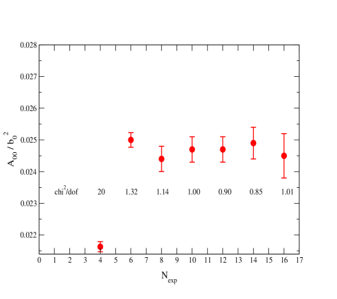
Figure 1: Fit results for $\frac{A_{00}}{b_{0}^{2}}$ versus the number of exponentials $N_{exp}=N+\tilde{N}$ for one of the coarse ensembles, Set C2 with $au_{0}m_{val}=0.04$.

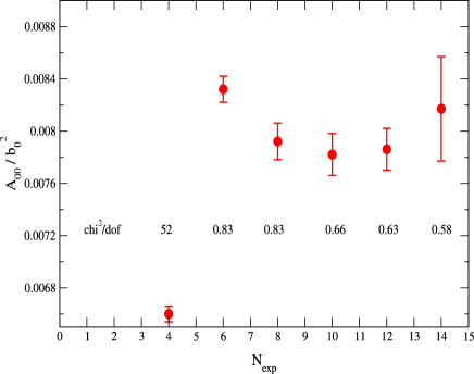
Figure 2: Same as Fig.1 for a fine ensemble, Set F1 with $au_{0}m_{val}=0.031$.

Our smearings consist of Gaussian smearings of the heavy quark propagator at both source and sink. In addition to point sources and sinks we use Gaussians with widths, in units of the lattice spacing, of 2.0 and 6.0 for sets C1 and C2 and one Gaussian each of width 6.0 for C3 and C4 and of width 8.0 for sets F1 and F2. To extract $\frac{A_{00}}{b_{0}^{2}}$ for our renormalized three-point function we carry out simultaneous fits to an $N_{sm}\times N_{sm}$ matrix of two-point correlators (eq.(III) with $\alpha,\beta=1,...N_{sm}$) ($\alpha=1$ corresponds to local, $\alpha=2$ to first Gaussian etc.) and to the renormalized three-point functions with $\alpha=\beta$. Bayesian fitting bayes methods are employed to enable these complicated fits with large numbers of exponentials, i.e. of fit parameters. We fit to all data points within $t_{min}\leq t\,,\,t_{1}\leq t_{max}$ and $t_{min}\leq t_{2}\leq t^{\prime}_{max}$ for $t_{min}=2\sim 3$, $t_{max}=20\sim 24$ and $t_{max}^{\prime}=13\sim 15$. We have used $N_{exp}\equiv N+\tilde{N}$ ranging between 4 to 16 and looked for consistency in fit results as the number of exponentials was increased. An example of fit results on one of the coarse lattices is shown in Fig.1. One sees that good and consistent results are obtained for $8\leq N_{exp}<16$. When $N_{exp}$ becomes very large (in the case of Fig.1 $\geq 16$), errors tend to increase again indicating that our fit ansatz has become too complicated for the minimization routines to handle, given the amount of statistics that we have. Fig.2 shows an example for one of the fine lattices. Here we find good results for $8\leq N_{exp}<14$. In general we have relied on our $N_{exp}=8,10$ and $12$ fits for all our ensembles.

We summarize fit results in Table II. The dimensionful quantities $f_{B_{q}}\sqrt{M_{B_{q}}\hat{B}_{B_{q}}}$ are given in units of $r_{1}^{-3/2}$. Errors include both statistical plus fitting errors and errors coming from uncertaintiy in $r_{1}/a$ which we take to be $\sim 0.5$%. Note that we have also gone to the renormalization group invariant bag parameter $\hat{B}_{B_{q}}$.

Table 2: Fit results for $f_{B_{q}}\sqrt{M_{B_{q}}\hat{B}_{B_{q}}}$ in units of $r_{1}^{-3/2}$ and for the dimensionless ratio $\xi\sqrt{\frac{M_{B_{s}}}{M_{B_{d}}}}=\frac{f_{B_{s}}\sqrt{B_{B_{s}}M_{B_{s}}}}{f_{B_{d}}\sqrt{B_{B_{d}}M_{B_{d}}}}$. Errors in the last column are statistical + fitting errors. Those in the second and third columns include additional errors coming from the 0.5% uncertainty in $r_{1}/a$.

Set	$r_{1}^{3/2}f_{B_{s}}\sqrt{M_{B_{s}}\hat{B}_{B_{s}}}$	$r_{1}^{3/2}f_{B_{d}}\sqrt{M_{B_{d}}\hat{B}_{B_{d}}}$	$\xi\sqrt{\frac{M_{B_{s}}}{M_{B_{d}}}}$
C1	1.430(21)	1.193(27)	1.199(29)
C2	1.442(16)	1.248(35)	1.155(33)
C3	1.382(21)	1.179(21)	1.172(23)
C4	1.413(18)	1.263(22)	1.119(22)
F1	1.353(17)	1.138(28)	1.189(26)
F2	1.334(20)	1.193(27)	1.118(24)

IV Chiral and Continuum Extrapolations

The lattice data presented in Table II are for simulations with $up$ and $down$ quark masses $m_{u}=m_{d}$ larger than in the real world and need to be extrapolated to the physical point. Reaching this physical point also involves taking the lattice spacing $a\rightarrow 0$ limit. We use staggered chiral perturbation theory (SChPT) schpt1 ; schpt2 ; schpt3 augmented by further general discretization correction terms to carry out the simultaneous chiral and continuum extrapolations. Continuum heavy meson chiral perturbation for $B$ and $D$ mixing was developed in detlin ; kamenik1 including for the partially quenched case. These formulas were generalized recently to next-to-leading order SChPT by Bernard, Laiho and Van de Water schpt4 and generously made available to us prior to publication. We use the following fit ansatz,

$$r_{1}^{3/2}\,f_{B_{q}}\sqrt{M_{B_{q}}\hat{B}_{B_{q}}}=$$

$$c_{1}\,[1+\frac{1}{2}\,\Delta f_{q}+c_{2}\,(2m_{f}+m_{s})\,r_{1}+c_{3}\,m_{q}\,r_{1}]\times$$

$$[1+c_{4}\,\alpha_{s}(a/r_{1})^{2}+c_{5}\,(a/r_{1})^{4}].$$ (18)

$\Delta f_{q}$ stands for the chiral log contributions and includes the staggered light quark action specific taste breaking terms. The factor of $1/2$ comes about since $\Delta f_{q}$ was calculated for the square, namely for $f^{2}_{B_{q}}M_{B_{q}}B_{B_{q}}$. We use the notation $m_{f}$ and $m_{s}$ for the sea $up/down$ and $strange$ quark masses respectively, and $m_{q}$ (or $m_{qs}$) for the valence quark masses. The second bracket parametrizes further discretization corrections that are expected to come in at ${\cal O}(\alpha_{s}\,a^{2})$ and ${\cal O}(a^{4})$. We have also tried adding more analytic terms with higher powers of quark masses.

$\Delta f_{q}$ includes the coupling $g_{B^{*}B\pi}$ which has not been measured experimentally. However, based on Heavy Quark Effective Theory (HQET) arguments, $g_{B^{*}B\pi}$ is believed to be close to an analogous coupling $g_{D^{*}D\pi}$ in the $D$ meson system for which some experimental information is available. The latter coupling is estimated to be between $0.3\leq g_{D^{*}D\pi}\leq 0.6$ gddpi . As we discuss below, we have carried out two types of fits, one where we did a whole sequence of fits with $g_{B^{*}B\pi}$ varying between $0\leq g_{B^{*}B\pi}\leq 0.6$ but where this coupling was kept fixed during each individual fit. In the second type of fit we let the coupling float and be one of the fit parameters. Both types of fits favored smaller values with $g_{B^{*}B\pi}\approx 0.1$, however as long as $g_{B^{*}B\pi}<0.5$ fit results were quite insensitive to its exact value.

For the ratio $\xi\sqrt{M_{B_{s}}/M_{B_{d}}}$ we use,

$$\xi\,\sqrt{\frac{M_{B_{s}}}{M_{B_{d}}}}=$$

$$[1+\frac{1}{2}\,(\Delta_{0}f_{qs}-\Delta_{0}f_{q})+\frac{b_{1}^{2}}{2}\,(\Delta_{1}f_{qs}-\Delta_{1}f_{q})+$$

$$b_{2}\,(m_{qs}-m_{q})\,r_{1}+b_{3}\,(m_{qs}-m_{q})^{2}\,r_{1}^{2}]\times$$

$$[1+(b_{4}\,\alpha_{s}(a/r_{1})^{2}+b_{5}\,(a/r_{1})^{4})(m_{qs}-m_{q})\,r_{1}].$$ (19)

Here we have split up,

$$\Delta f_{q}=\Delta_{0}f_{q}+g^{2}_{B^{*}B\pi}\,\Delta_{1}f_{q}$$ (20)

and then let $g_{B^{*}B\pi}\rightarrow b_{1}$ become one of the fit parameters. In Fig.3 we show a simultaneous fit to the six entries in the last column of Table II. The green and blue curves are the curves from this fit appropriate to the coarse and fine lattice data points respectively and the red curve is the “continuum” curve obtained by retaining the fitted values for $b_{1}$, $b_{2}$ and $b_{3}$ and turning off the $b_{4}$ and $b_{5}$ correction terms plus the taste breaking contributions inside $\Delta f_{q}$ and $\Delta f_{qs}$. One sees that within our statistical and fitting errors of $\sim 2$%, there is consistency between the three curves. In other words, we see almost no statistically significant lattice spacing dependence in this ratio. At the physical point the difference between the green and blue curves is 1.8%, which reduces to 1.3% if the green curve is adjusted and corrected for having a sea $strange$ quark mass on the coarse lattices that is about 20% too large. One might be surprised that the magenta curve lies below the blue curve. This comes about because the various discretization effects inside $(\Delta f_{qs}-\Delta f_{q})$ and in the $b_{4}$ & $b_{5}$ terms can have different signs and come in with different relative weights between the coarse and fine lattices. All these effects come in at the $\sim 0.5$% or less level, and are hence too small to allow us to disentangle one from the other in a meaningful way. The fit shown in Fig.3 has $\chi^{2}_{aug}/dof=0.54$ bayes2 and gives $g_{B^{*}B\pi}=0.14(47)$.

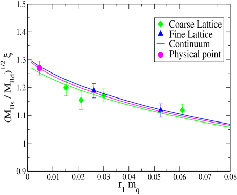
Figure 3: Chiral and continuum extrapolation of the ratio $\xi\sqrt{\frac{M_{B_{s}}}{M_{B_{d}}}}$. Errors shown are statistical plus fitting errors. The physical point is at $r_{1}m_{qs}/27.4$, where $m_{qs}$ is the valence strange quark mass.

Fig.4 shows chiral & continuum extrapolation curves for $r_{1}^{3/2}f_{B_{d}}\sqrt{\hat{B}_{B_{d}}M_{B_{d}}}$ using the fit ansatz of eq.(IV). Again the green and blue full curves are the fit curves for the coarse and fine lattice data respectively, and the dotted lines show the error bands around these central curves. Turning off the $c_{4}$ and $c_{5}$ contributions and the taste breaking terms inside $\Delta f_{q}$ leads to the red curve which can be followed down to the physical point. In contrast to the situation for the ratio $\xi$, here, with $f_{B_{d}}\sqrt{\hat{B}_{B_{d}}M_{B_{d}}}$, one finds a noticeable shift between the coarse and fine lattice points. The difference between the green and blue curves is a 5.5% effect. Going from the fine (blue) curve to the red continuum extrapolated curve is a 4% shift, which is also the size of the chiral & continuum extrapolation error at the physical point. The fit in Fig.4 has $\chi^{2}_{aug}/dof=0.99$.

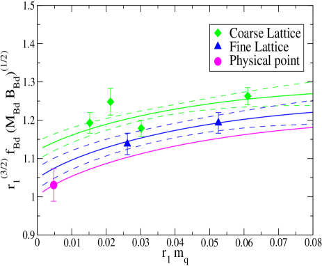
Figure 4: Chiral and continuum extrapolation of $r_{1}^{3/2}f_{B_{d}}\sqrt{\hat{B}_{B_{d}}M_{B_{d}}}$. Errors on the data points are statistical plus fitting errors combined with uncertainty in $r_{1}/a$. The dashed curves correspond to the error bands about the central green and blue full lines. The physical point is at $r_{1}m_{qs}/27.4$, where $m_{qs}$ is the valence strange quark mass.

Finally, in Fig.5 we show results for $r_{1}^{3/2}f_{B_{s}}\sqrt{\hat{B}_{B_{s}}M_{B_{s}}}$, where $\chi^{2}_{aug}/dof=0.96$ for the simultaneous fit to all the data points. Here the difference between the green and blue curves is a 6% effect and between the blue and red curve a 5.7% effect. These shifts are slightly larger than but similar to those for $B_{d}$ in Fig.4. In both cases the discretization effects we are seeing in $r_{1}^{3/2}f_{B_{q}}\sqrt{\hat{B}_{B_{q}}M_{B_{q}}}$ are larger than the naive expectation of a leading correction of ${\cal O}(a^{2}\alpha_{s})$ which would be $\sim 4$% or $\sim 2$% on the coarse or fine lattices respectively. It was hence very important to have simulations results at more than one lattice spacing and carry out an explicit continuum extrapolation. Fortunately, for the important ratio $\xi$ these discretization corrections cancel out to a large extent, as expected and as we have already verified in Fig.3.

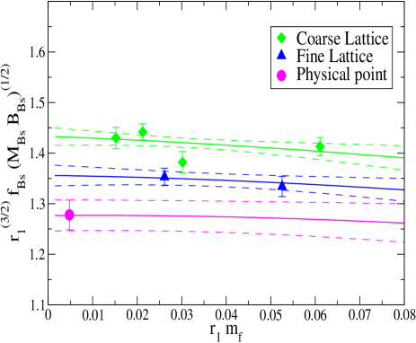
Figure 5: Same as Fig.4 for $r_{1}^{3/2}f_{B_{s}}\sqrt{\hat{B}_{B_{s}}M_{B_{s}}}$ versus $r_{1}m_{f}$.

V Main Results and Error Budget

Table III gives our error budget for the main uncertainties in the three quantities, $f_{B_{s}}\sqrt{\hat{B}_{B_{s}}}$, $f_{B_{d}}\sqrt{\hat{B}_{B_{d}}}$ and $\xi$.

Table 3: Errors in % for $f_{B_{s}}\sqrt{\hat{B}_{B_{s}}}$, $f_{B_{d}}\sqrt{\hat{B}_{B_{d}}}$ and $\xi$.

source of error	$f_{B_{s}}\sqrt{\hat{B}_{B_{s}}}$	$f_{B_{d}}\sqrt{\hat{B}_{B_{d}}}$	$\;\;\xi\;\;$
stat. + chiral extrap.	2.3	4.1	2.0
residual $a^{2}$ extrap.	3.0	2.0	0.3
uncertainty
$r_{1}^{3/2}$ uncertainty	2.3	2.3	—
$g_{B^{*}B\pi}$ uncertainty	1.0	1.0	1.0
$m_{s}$ and $m_{b}$ tuning	1.5	1.0	1.0
operator matching	4.0	4.0	0.7
relativistic corr.	2.5	2.5	0.4
Total	6.7	7.1	2.6

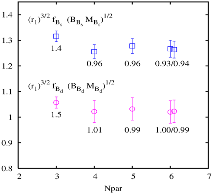
Figure 6: $r_{1}^{3/2}f_{B_{q}}\sqrt{\hat{B}_{B_{q}}M_{B_{q}}}$ at the physical point versus $Npar$, the number of fit parameters. The numbers below the data points give $\chi^{2}_{aug}/dof$. For $Npar=6$ we give results for two different types of term added, a term proportional to the quark mass squared (right data point) or a further discretization correction $\propto(a/r_{1})^{3}\alpha_{s}$ (left data point).

We explain each entry in Table III in turn.

• statistics and chiral extrapolations: These are the errors shown on the “physical points” in Figs.3, 4 and 5 and are outputs from our chiral & continuum extrapolation fits.

• residual $a^{2}$ extrapolation error: It is necessary to list this error separately since the degree to which the red curves in the above figures actually correspond to the true continuum limit depends on how well one has modelled discretization errors in our simulations. In other words one needs to assess the error in the fit ansatz for the continuum extrapolation (we assume the chiral extrapolation is handled sufficiently accurately by Staggered ChPT) and this turns out to be a nontrivial task.
  On the one hand the data appears to be consistent with the fit ansätze of eqs.(IV) and (IV). We have tried adding further terms and found that fit results shifted by an amount less than, and in most cases much less than, the “statistical + chiral extrapolation” errors. Fig.6 shows results for the chirally and continuum extrapolated $r_{1}^{3/2}f_{B_{q}}\sqrt{\hat{B}_{B_{q}}M_{B_{q}}}$ versus the number of parameters $Npar$ in the fit ansatz. For $Npar=3$ one has discretization corrections only through the $\Delta f_{q}$ $S\chi PT$ term and one sees that a good fit to the data points at the two lattice spacings cannot be obtained. However, once $Npar>3$, good fits are achieved and results and their errors are stable with respect to changes in $Npar$.
  On the other hand we know that due to our use of the NRQCD action to describe the heavy $b$ quark, coefficients such as $c_{4}$ are in general complicated functions of $(aM)$ (although $c_{4}$ does include a constant piece coming from the light quarks).
  We have approached this complicated situation in the following way. We interpret the red “continuum” curves in Figs.3, 4 and 5 as the curves one would get after taking care of all discretization errors coming from the light quark and the glue sectors. Then under “residual $a^{2}$ extrapolation uncertainty” one would include errors coming from the heavy quark action. The leading such error in our calculations is of ${\cal O}(a^{2}\alpha_{s})$ multiplied by some function of $(aM)$ which we initially take to be of ${\cal O}(1)$ leading to an additional uncertainty of $\sim 2$% in $f_{B_{q}}\sqrt{\hat{B}_{B_{q}}}$. This would correspond to a standard power counting estimate of discretization errors where one takes coefficients of order one in higher order corrections. We have opted to be slightly more conservative in our power counting assessment and apply a factor of 1.5 rather than 1.0 for those cases where the “physical” (the magenta) points deviate by more than one $\sigma$ from the fine lattice (blue) curve. By “$\sigma$” we mean here the “statistical + chiral extrapolation” errors. For $\xi$ we have multiplied the error for $f_{B_{d}}\sqrt{\hat{B}_{B_{d}}}$ by a factor of $\frac{(m_{s}-m_{u/d})}{\Lambda_{QCD}}\sim 1/6$.
  Since the second row in Table III gives an assessment of the uncertainty in our $a^{2}$ extrapolation rather than an estimate of the full discretization error, we believe the procedure outlined here to fix it is a reasonably conservative one.

• $r_{1}^{3/2}$ uncertainty: follows from the 1.5% error in current determinations of the physical value for $r_{1}$.

• uncertainty in $g_{B^{*}B\pi}$: we carried out fixed coupling chiral fits for the range $0.0<g_{B^{*}B\pi}<0.6$ and looked at the spread in the results at the physical point. For couplings larger than 0.6, $\chi^{2}/dof$ starts to deteriorate.

• tuning of strange and bottom quark masses: The largest mistuning, which occurs in the sea strange quark mass $m_{s}$ on the coarse lattices, has been corrected for when calculating fit results at the physical point and residual effects have been estimated by varying this adjusted value for $m_{s}$. Errors due to uncertainty in the valence $strange$ quark mass have been assessed by comparing $f_{B_{q}}\sqrt{\hat{B}_{B_{q}}}$ as one goes from valence quark mass $m_{qs}$ down to $m_{q}$ and errors coming from mistuning of $m_{b}$ have been estimated from the $1/M$ dependence of decay constants studied in fbsprl .

• operator matching and relativistic corrections: These two sources of error are intimately intertwined and again how to separate the two is not clear cut. As indicated in eq.(II), our matching for $f^{2}_{B_{q}}\hat{B}_{B_{q}}$ has been carried out up to correction of ${\cal O}(\alpha_{s}^{2})$ and ${\cal O}(\alpha_{s}\Lambda_{QCD}/M)$. In Table III we have listed the first correction under “operator matching” and the latter correction under “relativistic corrections”. And again the errors for $\xi$ are reduced by a factor of 1/6 relative to those for the two non ratio quantities.

Using central values coming from the physical (red) points in the figures and the errors summarized in Table III, we can now present our main results.

$$\xi\equiv\frac{f_{B_{s}}\sqrt{B_{B_{s}}}}{f_{B_{d}}\sqrt{B_{B_{d}}}}=1.258(25)(21),$$ (21)

and using $r_{1}=0.321(5)fm$ upsilon ,

$$f_{B_{s}}\sqrt{\hat{B}_{B_{s}}}=266(6)(17)\;\left(\frac{0.321}{r_{1}[fm]}\right)^{3/2}{\rm MeV},$$ (22)

$$f_{B_{d}}\sqrt{\hat{B}_{B_{d}}}=216(9)(12)\;\left(\frac{0.321}{r_{1}[fm]}\right)^{3/2}{\rm MeV},$$ (23)

where the first error comes from statistics + chiral extrapolation and the second is the sum of all other systematic errors added in quadrature. From the individual $f_{B_{q}}\sqrt{\hat{B}_{B_{q}}}$, q=s or d, one obtains a ratio of 1.231(58)(21) which is consistent with (21) however with larger errors. The result for $f_{B_{s}}\sqrt{\hat{B}_{B_{s}}}$ in eq.(22) is consistent with but more accurate than our previously published value of $281(21)$MeV bsmixing .

VI Updates on $f_{B_{d}}$, $f_{B_{s}}$ and $f_{B_{s}}\,/\,f_{B_{d}}$ and Estimates of Bag Parameters

The numerical simulations of two-point and three-point functions, such as in eqns.(III) and (III), that enabled us to extract the B-mixing parameters of the previous section also provide information necessary to determine $B_{d}$ and $B_{s}$ meson decay constants $f_{B_{d}}$ and $f_{B_{s}}$. Decay constants are defined through the matrix element of the heavy-light axial vector current between the $B_{q}$ meson state and the hadronic vacuum. Using the temporal component $A_{0}$ and working in the heavy meson rest frame one has,

$$\langle 0|A_{0}|B_{q}\rangle\equiv M_{B_{q}}f_{B_{q}}.$$ (24)

Just as with the four-fermion operators of section II, matching is required between the heavy-light current in continuum QCD and currents made out of quark fields of the effective lattice theory. This matching has been carried out at the one-loop order for NRQCD/AsqTad currents in pert1 based on formalism developed in pert2 .

$$\langle\,A_{0}\,\rangle^{\overline{\rm MS}} = (1+\alpha_{s}\,\tilde{\rho}_{0})\,\langle J^{(0)}_{0}\rangle+$$ (25)

$$(1+\alpha_{s}\,\rho_{1})\,\langle J^{(1),sub}_{0}\rangle\;+\;\alpha_{s}\,\rho_{2}\,\langle J^{(2),sub}_{0}\rangle$$

$$+ \quad{\cal O}(\alpha_{s}^{2},\Lambda_{QCD}^{2}/M^{2})\,,$$

The heavy-light currents $J_{0}^{(i)}$ in the effective theory are defined as,

$$J^{(0)}_{0} = \overline{\Psi}_{q}\,\Gamma_{0}\,\Psi_{Q},$$ (26)

$$J^{(1)}_{0} = \frac{-1}{2\,(aM)}\overline{\Psi}_{q}\,\Gamma_{0}\,\mbox{\boldmath$\gamma\!\cdot\!\nabla$}\,\Psi_{Q},$$ (27)

$$J^{(2)}_{0} = \frac{-1}{2\,(aM)}\overline{\Psi}_{q}\,\mbox{\boldmath$\gamma\!\cdot\!\overleftarrow{\nabla}$}\,\gamma_{0}\ \Gamma_{0}\,\Psi_{Q}.$$ (28)

with $\Gamma_{0}\equiv\gamma_{5}\gamma_{0}$ and

$$J_{0}^{(i),sub}\equiv J_{0}^{(i)}-\alpha_{s}\,\zeta_{i0}\,J_{0}^{(0)}$$ (29)

The matching coefficients $\rho_{i}$ and $\zeta_{i0}$ are given in pert1 . Note that the matching for the heavy-light current includes contributions at ${\cal O}(\alpha_{s}\frac{\Lambda_{QCD}}{M})$ and hence is more accurate than the matching in (II) for the four-fermion operator.

Table 4: Fit results for $\Phi_{q}=f_{B_{q}}\sqrt{M_{B_{q}}}$ in units of $r_{1}^{-3/2}$ and for the ratio $\Phi_{s}/\Phi_{d}$. Errors are as described in Table II.

Set	$\quad r_{1}^{3/2}\Phi_{s}\quad$	$\quad r_{1}^{3/2}\Phi_{d}\quad$	$\quad\Phi_{s}/\Phi_{d}\quad$
C1	1.261(12)	1.085(14)	1.162(14)
C2	1.246(11)	1.073(14)	1.162(12)
C3	1.236(12)	1.071(14)	1.155(14)
C4	1.248(16)	1.128(17)	1.107(20)
F1	1.175(13)	0.990(22)	1.188(20)
F2	1.180(13)	1.047(16)	1.120(11)

We have evaluated the two-point functions,

$$C^{2pt}_{j\beta}(t)=\sum_{\vec{x}_{1},\vec{x}_{2}}\langle 0|J_{0}^{(j)}(\vec{x}_{1},t)\;\Phi^{\beta\dagger}_{B_{q}}(\vec{x}_{2},0)|0\rangle$$ (30)

for $j=0,1,2$. We then calculate the renormalized current matrix element by forming the appropriate linear combination as dictated by the RHS of (25). This is done for both $B_{d}$ and $B_{s}$. The next step is to fit the renormalized two-point correlator using the ansatz of eq.(III), extract the relevant ground state matrix element and thereby obtain $\Phi_{q}\equiv f_{B_{q}}\sqrt{M_{B_{q}}}$. We do simultaneous fits to $B_{d}$ and $B_{s}$ correlators, so that $\Phi_{d}$, $\Phi_{s}$ and the ratio $\Phi_{s}/\Phi_{d}$ are determined within the same fit. Fit results are summarized in Table IV. For $r_{1}^{3/2}\Phi_{q}$ errors include the uncertainty in $r_{1}/a$ in addition to statistical and fitting errors.

The rest of the analysis for $\Phi_{q}$ and $\Phi_{s}/\Phi_{d}$ is very similar to what was done for the four-fermion operator matrix elements in section IV. Chiral and continuum extrapolations are carried out using a fit ansatz of the form (IV) for $r_{1}^{3/2}\Phi_{q}$ and (IV) for $\Phi_{s}/\Phi_{d}$. The only difference is that here $\Delta f_{q}$ will involve the chiral logarithms appropriate for decay constants rather than for four-fermion operators. Such contributions were calculated by Aubin & Bernard using Staggered ChPT in reference schpt3 . Fig.7, 8 and 9 show chiral and continuum extrapolations for $\Phi_{s}/\Phi_{d}$, $\Phi_{d}$ and $\Phi_{s}$ with $\chi^{2}_{aug}/dof$ = 1.00, 1.06 and 0.53 respectively.

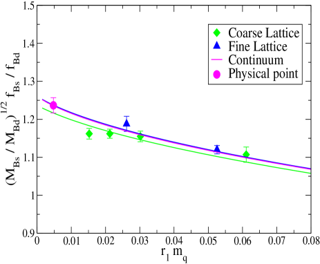
Figure 7: Chiral and continuum extrapolation of the ratio $\Phi_{s}/\Phi_{d}$. The different curves and the physical point have same meanings as in Fig.3. Here the red (continuum) curve is essentially on top of the blue (fine lattice) curve.

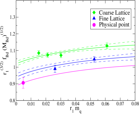
Figure 8: Same as Fig.4 for $r_{1}^{3/2}\Phi_{d}=r_{1}^{3/2}f_{B_{d}}\sqrt{M_{B_{d}}}$.

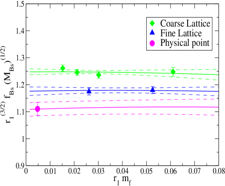
Figure 9: Same as Fig.5 for $r_{1}^{3/2}\Phi_{s}=r_{1}^{3/2}f_{B_{s}}\sqrt{M_{B_{s}}}$.

Table 5: Errors in % for $f_{B_{s}}$, $f_{B_{d}}$ and $f_{B_{s}}/f_{B_{d}}$.

source of error	$\quad f_{B_{s}}\quad$	$\quad f_{B_{d}}\quad$	$\;\;f_{B_{s}}/f_{B_{d}}\;\;$
stat. + chiral extrap.	2.2	3.5	1.6
residual $a^{2}$ extrap.	3.0	3.0	0.5
uncertainty
$r_{1}^{3/2}$ uncertainty	2.3	2.3	—
$g_{B^{*}B\pi}$ uncertainty	1.0	1.0	0.3
$m_{s}$ and $m_{b}$ tuning	1.5	1.0	1.0
operator matching	4.0	4.0	0.7
relativistic corr.	1.0	1.0	0.2
Total	6.3	6.7	2.1

Table V shows the error budget for $f_{B_{s}}$, $f_{B_{d}}$ and $f_{B_{s}}/f_{B_{d}}$, which is very similar to Table III for the mixing parameters. The meaning of the different sources of error is as explained in section V. We have mentioned already that ${\cal O}(\alpha_{s}\frac{\Lambda_{QCD}}{M})$ effects in the matching of the heavy-light current have been taken into account in our one-loop matching calculations pert1 . Hence, these should not be included under “relativistic corrections” in Table V. However, there are still ${\cal O}(\alpha_{s}\frac{\Lambda_{QCD}}{M})$ corrections to worry about in the NRQCD action. These would come from radiative corrections to the coefficient $c_{B}$ (often also denoted $c_{4}$) of the $\frac{1}{2M}\,\mbox{\boldmath$\sigma$}\cdot{\bf B}$ term in the action. Although one-loop corrections to $c_{B}$ have not been calculated yet, one can nevertheless bound this coefficient nonperturbatively by calculating the hyperfine, the $B^{*}-B$, splitting and comparing with experiment. Preliminary results discussed in upsilon indicate that $c_{B}$ is close to one and the entire effect would be at most a 10% correction to a $\frac{\Lambda_{QCD}}{M}$ contribution. For the present calculations this means an uncertainty of order 1% in $f_{B_{q}}$ and a much smaller one for $\frac{f_{B_{s}}}{f_{B_{d}}}$.

The final numbers for the decay constants including all errors added in quadrature become,

$$\frac{f_{B_{s}}}{f_{B_{d}}}=1.226(26),$$ (31)

$$f_{B_{d}}=190(13)\;\left(\frac{0.321}{r_{1}[fm]}\right)^{3/2}{\rm MeV},$$ (32)

and

$$f_{B_{s}}=231(15)\;\left(\frac{0.321}{r_{1}[fm]}\right)^{3/2}{\rm MeV}.$$ (33)

These results for $f_{B_{q}}$ are consistent with but about one $\sigma$ lower than the values $f_{B_{d}}=216(22)$MeV and $f_{B_{s}}=260(29)$MeV given in fbprl ; fbsprl . The main difference between the analysis carried out here and in fbprl is that in the latter case chiral extrapolations were done based only on coarse lattice data and furthermore no attempt was made to extrapolate explicitly to the continuum limit. The new result for the ratio in (31) is similarly consistent with our previous $f_{B_{s}}/f_{B_{d}}=1.20(3)(1)$ fbprl .

The $B_{q}$ mixing simulations can also be used to determine the bag parameters $B_{B_{q}}$. From the separate final results for $f_{B_{q}}\sqrt{B_{B_{q}}}$ and for $f_{B_{q}}$ one finds $B_{B_{s}}(\mu=M_{b})=0.86(6)$ and $B_{B_{d}}(M_{b})=0.84(10)$. We have also attempted to extract the bag parameters directly from simultaneous fits to 3-point and 2-point correlators for each ensemble separately. The results are shown for $\hat{B}_{B_{s}}$ in Fig.10 and extrapolated to the physical point, where one finds $\hat{B}_{B_{s}}=1.33(5)$. We add to this 3.8% statistical + chiral extrapolation error additional 2.5% systematic errors. Many of the systematic errors listed in Tables III and V are either irrelevant or cancel to a large extent in $\hat{B}_{B_{s}}$. For instance, one sees from Fig.10 that there is little evidence for discretization errors in the bag parameter, although $f_{B_{s}}\sqrt{M_{B_{s}}B_{B_{s}}}$ and $f_{B_{s}}\sqrt{M_{B_{s}}}$ individually do have noticeable lattice spacing dependence. Our final result for the $B_{s}$ meson bag parameter is $\hat{B}_{B_{s}}=1.33(6)$, or $B_{B_{s}}(M_{b})=0.86(4)$. One sees that direct extraction of the bag parameter followed by a continuum/chiral extrapolation can reduce errors significantly over our first approach of extrapolating $f_{B_{s}}\sqrt{M_{B_{s}}B_{B_{s}}}$ and $f_{B_{s}}\sqrt{M_{B_{s}}}$ first and then taking the ratio. Although we were successful in applying the second method for $B_{B_{s}}$, unfortunately it has not been possible to get stable extractions of $B_{B_{d}}$ for all of our six ensembles. Our best estimate for the $B_{d}$ meson bag parameter is obtained by taking the two ratios, $f_{B_{s}}\sqrt{B_{B_{s}}}/f_{B_{d}}\sqrt{B_{B_{d}}}$ and $f_{B_{s}}/f_{B_{d}}$, from eqs.(21) and (31) and combining their ratio with our most accurate $B_{B_{s}}(M_{b})$. This leads to $B_{B_{s}}/B_{B_{d}}=1.05(7)$ and $B_{B_{d}}(M_{b})=0.82(7)$.

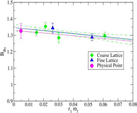
Figure 10: Chiral and continuum extrapolation of the bag parameter $\hat{B}_{B_{s}}$. In order to avoid clutter, we show an error band only for the fit to the coarse lattice data.

VII Summary

We have completed the first $N_{f}=2+1$ unquenched study of $B_{s}$ and $B_{d}$ mixing phenomena in Lattice QCD. Our main results, namely values for $\xi=\frac{f_{B_{s}}\sqrt{B_{B_{s}}}}{f_{B_{d}}\sqrt{B_{B_{d}}}}$, $f_{B_{s}}\sqrt{\hat{B}_{B_{s}}}$ and $f_{B_{d}}\sqrt{\hat{B}_{B_{d}}}$, are given in eqns.(21), (22) and (23) respectively. Combining the lattice result for $\xi$ with the experimentally measured mass differences $\Delta M_{d}=0.507\pm 0.005\;ps^{-1}$ pdg and $\Delta M_{s}=17.77\pm 0.10\pm 0.07\;ps^{-1}$ cdf leads to,

$$\frac{|V_{td}|}{|V_{ts}|}=0.214(1)(5)$$ (34)

where the first error is experimental and the second from the lattice calculation presented here. This is the first time this ratio of CKM matrix elements has been determined while incorporating a fully self consistent $N_{f}=2+1$ calculation of $\xi$.

In addition to giving mixing parameter results, in this article we have also updated values for decay constants $f_{B_{d}}$ and $f_{B_{s}}$ and their ratio in section VI. $f_{B_{s}}$ appears in the Standard Model prediction for the branching fraction for $B_{s}\rightarrow\mu^{+}\mu^{-}$ bb , a process sensitive to new physics. The most accurate result for this branching fraction comes from taking a ratio with $\Delta M_{s}$ buras2 , which gives a result inversely proportional to $\hat{B}_{B_{s}}$. Updating the parameters used in buras2 for $\tau(B_{s})$ and $\overline{m_{t}}$ pdg , and including our result for $\hat{B}_{B_{s}}$ of 1.33(6), gives

$$Br(B_{s}\rightarrow\mu^{+}\mu^{-})=3.19(19)\times 10^{-9},$$ (35)

improving on the previous accuracy available. The largest contribution to the error on the branching fraction comes from the error on $\hat{B}_{B_{s}}$ followed by the uncertainty in $\tau(B_{s})$.

The calculations presented here can be improved in several ways. Foremost among the improvements planned for the future is to carry out simulations at other, finer, lattice spacings. Having results at more than two lattice spacings will help considerably in reducing the “statistical + chiral extrapolation” and the “residual $a^{2}$ extrapolation” uncertainties in Tables III & V. They would also contribute to constraining the value of $g_{B^{*}B\pi}$ so that this source of error can then be ignored. Hence, one can expect lattice results for $\xi$ (and also for $f_{B_{s}}/f_{B_{d}}$) with accuracy of $\sim 1$% in the not too distant future. Improvement for dimensionful quantities such as $f_{B_{q}}\sqrt{\hat{B}_{q}}$ will also require reducing the “$r_{1}^{3/2}$” and the “operator matching” errors. The HPQCD collaboration is currently engaged in projects aimed at fixing the physical value of $r_{1}$ hpqcd1 with higher precision than in the past. We are also exploring nonperturbative methods for carrying out operator matching in heavy-light systems. At least for heavy-light currents, methods recently applied to accurate determinations of heavy quark masses, which involve moments of current correlators and very high order continuum QCD perturbation theory hpqcd2 , look promising for nonperturbative determinations of $Z$-factors. More work will be necessary to see whether such methods can be generalized to four-fermion operators. It is possible one can take advantage of the fact that a major contribution to matching of four-fermion operators comes from diagrams involving radiative corrections to just one of the bilinears within the four-fermion operator, in other words corrections that are identical to a heavy-light current radiative correction. This has been noted already in the one-loop calculations of fourfmatch . With several of these improvements in place better than $\sim 5$% accuracy should be achievable for $f_{B_{q}}\sqrt{\hat{B}_{B_{q}}}$.

Another worthwhile direction for future investigations would be to calculate hadronic matrix elements of further $\Delta B=2$ four-fermion operators, beyond the two, $OL$ and $OS$, studied here. As is well known, there are five such operators usually denoted $Qi$, with $i=1,2,3,4,5$ gabbiani ; becirevic ; fourfmatch . In this notation $OL\equiv Q1$ and $OS\equiv Q2$. In this article we have focused on $Q1$ and $Q2$ since only they are relevant for the mass difference $\Delta M_{q}$ in the Standard Model. The operator $Q3$ would come in for calculations of the width difference $\Delta\Gamma_{q}$ lenz . Although we have already accumulated simulation data for $\langle Q3\rangle$ we will postpone analysis for a future publication where we also plan to have results for $\langle Q4\rangle$ and $\langle Q5\rangle$. In fourfmatch the necessary matching at one loop has already been completed for all five four-fermion operators. The two hadronic matrix elements $\langle Q4\rangle$ and $\langle Q5\rangle$ do not appear in the Standard Model but are of interest in several Supersymmetric Models. To date only quenched lattice results exist for all five four-fermion operators becirevic . It will be important for Beyond the Standard Model studies to generalize those results to unquenched calculations.

Acknowledgments:
This research was supported by the DOE and NSF (USA), the STFC, Royal Society and Leverhulme Trust (UK), and by the Junta de Andalucía (Spain). Numerical work was carried out on facilities of the USQCD Collaboration funded by the Office of Science of the U.S. DOE. We are grateful to the MILC collaboration for making their gauge configurations available and for updates on $r_{1}/a$. We thank Claude Bernard, Jack Laiho and Ruth Van de Water for providing their results on Staggered ChPT for four-fermion operators prior to publication.

References

- (1) C.Amsler et al. Review of Particle Physics, Phys. Lett. B667:1, 2008.
- (2) A.Abulencia et al. [CDF Collaboration]; Phys. Rev. Lett. 97, 242003 (2006).
-
(3)
V.Abazov et al. [DØ Collaboration];
Phys. Rev. Lett. 97, 021802 (2006);
DØ note 5618-CONF (2008). - (4) C.Bernard et al.; Phys. Rev. D64, 054506 (2001).
- (5) Updated but unpublished numbers were obtained from the Fermilab Lattice and MILC Collaborations website. We thank the MILC collaboration for making this information available.
- (6) A.Gray et al. [HPQCD Collaboration]; Phys. Rev. D72, 094507 (2005).
- (7) C.Aubin et al.; Phys. Rev. D70, 031504 (2004).
- (8) Y.Shamir; Phys. Rev. D75, 054503 (2007); C.Bernard, M.Golterman and Y.Shamir; Phys. Rev. D77, 074505 (2007); M.Creutz; PoS LAT2007:007, 2007.
-
(9)
S.Sharpe; PoS LAT2006: 022 (2006);
A.Kronfeld; PoS LAT2007: 016 (2007). - (10) E.Dalgic et al. [HPQCD Collaboration]; Phys. Rev. D76, 011501(R) (2007).
- (11) S.Aoki et al. [JLQCD Collaboration]; Phys. Rev. Lett. 91, 212001 (2003).
- (12) R.T.Evans et al. [Fermilab Lattice and MILC Collaborations]; PoS LAT2008: 052 (2008).
- (13) E.Gámiz; Plenary Talk presented at Lattice 2008; arXiv:0811.4146 [hep-lat].
- (14) A.Gray et al. [HPQCD Collaboration]; Phys. Rev. Lett. 95, 212001 (2005).
- (15) M.Wingate et al. [HPQCD Collaboration]; Phys. Rev. Lett. 92, 162001 (2004).
- (16) A.J.Buras, M.Jamin and P.Weisz; Nucl.Phys. B347, 491 (1990).
-
(17)
G.P.Lepage; Phys. Rev. D59, 074501 (1999);
K.Originos, D.Toussaint and R.L.Sugar; ibid. 60, 054503 (1999); C.Bernard et al. [MILC Collaboration]; ibid. 61, 111502 (2000). - (18) G.P.Lepage et al.; Phys. Rev. D46, 4052 (1992).
- (19) E.Gámiz, J.Shigemitsu and H.Trottier; Phys. Rev. D77, 114505 (2008).
- (20) G.P.Lepage et al. [HPQCD Collaboration]; Nucl. Phys. B (Proc. Suppl.)106, 12 (2002).
- (21) W.Lee and S.Sharpe; Phys. Rev. D60, 114503 (1999).
- (22) C.Bernard; Phys. Rev. D65, 054031 (2002); C.Aubin and C.Bernard; Phys. Rev. D68, 034014 & 074011 (2003).
- (23) C.Aubin and C.Bernard; Phys. Rev. D73, 014515 (2006).
- (24) W.Detmold and C.J.Lin; Phys. Rev. D76, 014501 (2007).
- (25) D.Becirevic, S.Fajfer and J.F.Kamenik; JHEP 0706:003 (2007).
- (26) C.Bernard, J.Laiho and R.Van de Water; Fermilab Lattice and MILC collaborations internal memo, October 2007.
-
(27)
I.W.Stewart; Nucl.Phys. B529, 62 (1998);
M.C.Arnesen et al.;
Phys. Rev. Lett. 95, 071802 (2005);
S.Fajfer and J.F.Kamenik; Phys. Rev. D74, 074023 (2006). - (28) See reference bayes for a definition of . Note also that with Bayesian fits “dof” equals the number of data points (and not number of data points minus the number of fit parameters) as explained after eq.(8) of this same reference.
- (29) E.Gulez, J.Shigemitsu and M.Wingate; Phys. Rev. D69; 074501 (2004).
- (30) C.Morningstar and J.Shigemitsu; Phys. Rev. D57, 6741 (1998).
- (31) G.Buchalla and A.Buras; Nucl.Phys. B400, 225 (1993).
- (32) A.Buras; Phys.Lett. B 566, 115 (2003).
- (33) I.Kendall et al. [HPQCD Collaboration]; Talk presented at Lattice 2008.
- (34) I.Allison et al. [HPQCD Collaboration]; Phys. Rev. D78, 054513 (2008); C.Davies, G.P.Lepage et al. [HPQCD Collaboration]; arXiv:0810.3548 [hep-lat].
- (35) F.Gabbiani et al.; Nucl.Phys. B477, 321 (1996).
- (36) D.Becirevic et al.; JHEP 0204:025 (2002).
- (37) A.Lenz and U.Nierste; JHEP 0706:072 (2007).