Asymmetric Exclusion Processes with Disorder: Effect of Correlations

Abstract

Multi-particle dynamics in one-dimensional asymmetric exclusion processes with disorder is investigated theoretically by computational and analytical methods. It is argued that the general phase diagram consists of three non-equilibrium phases that are determined by the dynamic behavior at the entrance, at the exit and at the slowest defect bond in the bulk of the system. Specifically, we consider dynamics of asymmetric exclusion process with two identical defect bonds as a function of distance between them. Two approximate theoretical methods, that treat the system as a sequence of segments with exact description of dynamics inside the segments and neglect correlations between them, are presented. In addition, a numerical iterative procedure for calculating dynamic properties of asymmetric exclusion systems is developed. Our theoretical predictions are compared with extensive Monte Carlo computer simulations. It is shown that correlations play an important role in the particle dynamics. When two defect bonds are far away from each other the strongest correlations are found at these bonds. However, bringing defect bonds closer leads to the shift of correlations to the region between them. Our analysis indicates that it is possible to develop a successful theoretical description of asymmetric exclusion processes with disorder by properly taking into account the correlations.

I Introduction

In recent years a significant attention has been devoted to investigation of low-dimensional asymmetric simple exclusion processes (ASEPs) derrida98 ; zia95 ; schutz ; chowdhury00 ; derrida93 . They play a critical role for understanding fundamental properties of non-equilibrium phenomena in Chemistry, Physics and Biology. ASEPs have been widely utilized for description of traffic phenomena chowdhury00 , kinetics of biopolymerization macdonald68 , protein synthesis shaw03 ; chou04 ; shaw04 ; dong07 , and biological transport of motor proteins lipowsky01 ; parmeggiani03 . The advantage of using asymmetric exclusion processes for studying mechanisms of non-equilibrium phenomena is due to the fact that some homogeneous versions of ASEPs can be solved exactly via matrix-product approach and related methods derrida98 ; derrida93 ; blythe07 . In addition, understanding of processes in ASEPs can be achieved by utilizing a phenomenological domain wall approach DW . In order to have a more realistic description of different non-equilibrium phenomena ASEPs with inhomogeneous distribution of rates are required. However, there is a limited number of studies dealing with ASEPs with disorder in the transition rates at sites (static impurities) chou04 ; shaw04 ; janowsky92 ; schutz93 ; schutz93PRE ; janowsky94 ; kolomeisky98 ; tripathy97 ; barma98 ; kolwanker ; ha ; stinchcombe ; derrida04 ; juhasz05 ; barma06 ; pierobon06 ; foulaadvand07 ; foulad07 ; dongPRE ; greulich1 ; greulich2 and with disorder associated to particles’s hopping rates (moving impurities) speers ; mallick ; evans ; kim ; fouladvand99 . In this case exact solutions are not obtained, and extensive Monte Carlo computer simulations and approximate theories are utilized in order to understand particle dynamics. Disorder has a strong effect on the behavior of ASEPs. Even a single defect bond far away from the boundaries lead to dramatic effects in the stationary properties both in closed janowsky92 ; janowsky94 and open boundary conditions kolomeisky98 . It was shown recently that the dynamics of ASEPs is also influenced by several defects that are close to each other chou04 ; dong07 ; greulich1 , although the mechanism of this phenomenon is not well understood. This interaction between defects is important for understanding several biological transport phenomena chou04 ; dong07 . Recently the particular case of two defects has been extensively investigated by Monte Carlo simulations dong07 . It has been shown that the system current exhibits a notable dependence on the distance between defects with equal hopping rates. Moreover, it was found that the density profile is linear between defects which marks the existence of wandering shock between defects dong07 . The case of two defective sites with equal rate has been generalized to include extended objects dongPRE . Theoretical efforts to analyze ASEPs with disorder have been mostly directed to the cases with a single or few defects kolomeisky98 ; chou04 ; greulich1 . In Ref. kolomeisky98 ASEP with open boundaries and with a local inhomogeneity in the bulk has been investigated by arguing that the defect bond divides the system into two coupled homogeneous ASEPs. This theoretical approach can be called a defect mean-field (DMF) because the mean-field assumptions are made only at the position of local inhomogeneity. Although a good agreement with computer simulations has been found, there were significant deviations in statistical properties of the phase with the maximal current that was attributed to the neglect of correlations at the defect bond in the proposed theory kolomeisky98 . A related approach called interacting subsystem approximation (ISA) has been proposed in Ref. greulich1 for ASEPs with a single defect or several consecutive defects (bottleneck). Here it was suggested that due to the defect bonds there are 3 segments in the system: two homogeneous ASEPs are coupled by a segment that includes all sites that surround defect bonds. Explicit results have been used inside the segments, and mean-field assumptions have been utilized for particle dynamics between the segments. A better agreement with Monte Carlo computer simulations has been found, and the method was also successfully applied to describe interactions of defects with boundaries. It was argued that ISA can be used for analyzing properties of general ASEPs with disorder greulich1 ; greulich2 . However, ISA has not been applied for the systems with 2 defects at finite distances from each other, and because of this observation it is difficult to apply ISA for understanding mechanisms of more complex inhomogeneous asymmetric exclusion processes. A slightly different method of calculations has been proposed by Chou and Lakatos chou04 , who applied a finite segment mean-field theory (FSMFT). According to this approach, the segment of finite length $n$ that covers the defect and surrounding sites is considered, and its dynamics is fully described by solving explicitly for eigenvectors of the corresponding transition rate matrix. The segment is then coupled in the mean-field fashion to the rest of the system. However, this approach becomes numerically quite involved for cluster sizes larger than $\approx$20, and it also limits its applicability. Different studies of asymmetric exclusion processes with disorder point out to importance of correlations in the system. It is reasonable to expect that correlations are stronger near the slow defect sites. However, it is not clear how far from the local inhomogeneity and how fast these correlations decay. In addition, it is also unclear how correlations from two close defects affect each other. The goal of this paper is to investigate the role of correlations in dynamics of ASEPs with disorder. By analyzing several analytical approaches in combination with extensive Monte Carlo computer simulations it will be shown that a successful description of disordered driven diffusive systems can be achieved by properly accounting for correlations near the defect bonds.

II Model and Theoretical Description

We investigate a totally asymmetric simple exclusion processes with disorder. In the one-dimensional lattice the particle at the site $i$ can jump forward with the rate $p_{i}$ if the next site $i+1$ is unoccupied, otherwise it stays at the same place. The particle can enter the system with the rate $\alpha$ if the site is empty, and it can also exit the lattice with the rate $\beta$. When all $p_{i}=1$ we have a homogeneous ASEP for which dynamic properties are known explicitly from exact solutions derrida98 ; schutz . ASEPs with disorder correspond to the situation when there is inhomogeneities in the transition rates, and $p_{i}$ are drawn from arbitrary distributions. Numerous theoretical and computational studies indicate that in the limit of large times the dynamics in the system can be determined by comparing entrance rate, exit rates and the transition rate at the slowest defect bond kolomeisky98 ; greulich2 . This observation has a significant consequence for properties of ASEPs with disorder, yielding a generic phase diagram with 3 phases. When the entrance is a rate-limiting process the system can be found in the low-density phase, while for slow exiting the high-density phase governs the system. If the rate-limiting process is the transition via the slowest defect bond the system is in the maximal-current phase. In this maximal-current phase, a segregation of density profile into macroscopic high and low regions occurs at the location of slowest defect bond. Other defects only perturb the density profile on a local scale. However, when the number slowest defect bonds exceeds two or more the above picture needs modification. Furthermore, the previous studies on disordered ASEPs lack investigations on correlation effects induced by defects. To address these questions, we analyze the simplest model with 2 identical defects in the bulk of the system far away from the boundaries. It was shown earlier greulich1 that positioning of the slow defects close to the boundaries leads only to rescaling of the effective entrance and/or exit rates, and we will not consider this possibility in this paper. Note that in this paper we are using terms of defect bonds and defect sites. To clarify, we define the defect site as the site $i$ from which the particle hopes to the site $i+1$ with the rate $q<1$. Correspondingly, the bond connecting sites $i$ and $i+1$ is a defect one.

II.1 Defect Mean-Field Theory

Consider a totally asymmetric exclusion processes with open boundaries and with 2 slow defective sites at $i=d_{1}$ and $i=d_{2}$ at a distance $d$ with $d_{2}-d_{1}=d$ (separated by $d-1$ normal sites), as shown in Fig. 1. At the defects the particle jump to the right with the rate $q<1$, in all other sites the hopping rate is equal to one. It can be seen that two defects divide the system into three segments.

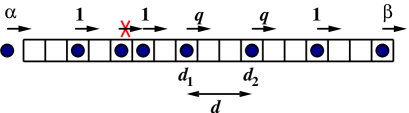
Figure 1: Fig.1: Schematic of ASEP with two defective sites at $i=d_{1}$ and $i=d_{2}$ separated by $d-1$ normal sites i.e., $d_{2}-d_{1}=d$. The reduced hopping rates at each defect is equal to $q$. In normal sites the hoping rates are one.

The particle dynamics inside each segment can be calculated exactly, however, it is assumed that there are no correlations between the segments. If entrance to the lattice is the slowest process then the system can be found in low-density (LD) phase with stationary current and bulk densities given by

$$J=\alpha(1-\alpha),\quad\rho_{bulk}=\alpha.$$ (1)

Similarly, when the exit becomes a bottleneck process the system is in high-density (HD) phase with

$$J=\beta(1-\beta),\quad\rho_{bulk}=1-\beta.$$ (2)

Note that in both phases particle densities near the defect bonds will deviate from the bulk values. The more interesting case is when the dynamics in the system is governed by transitions via local inhomogeneities. In this phase, which has the maximal current, we expect to have density phase segregation similar to the case a single defect ASEPs. We emphasize that all our investigation in this paper is on this maximal-current phase. First consider a lattice segment after the second defect. The dynamics in this part of the system is controlled by the entrance of particle via the defect, then it has a low-density profile with unknown bulk density $\rho^{*}<1/2$. Similar arguments can be used to analyze the density profile in the segment before the first defect. Here the flux is limited by the exit rate via the local inhomogeneity, leading to the high-density phase. Since at stationary-state condition the flux through any segment should be the same, $J=\rho^{*}(1-\rho^{*})$, the bulk density in this segment is equal to $1-\rho^{*}$. The region between two defects can be viewed as asymmetric exclusion process on a finite lattice with $d$ sites. The effective entrance and exit rates to this segment can be easily evaluated using our mean-field assumptions,

$$\alpha_{eff}=\beta_{eff}=q(1-\rho^{*}).$$ (3)

The stationary properties of the lattice segment with $d$ sites between the defects can be evaluated explicitly by utilizing exact results for finite-size ASEPs derrida93 . Specifically, the particle flux is given by

$$J_{0}(\alpha,\beta,d)=\frac{R_{d-1}(1/\beta)-R_{d-1}(1/\alpha)}{R_{d}(1/\beta)-R_{d}(1/\alpha)},$$ (4)

where the function $R_{d}(x)$ is defined as

$$R_{d}(x)=\sum_{p=2}^{d+1}\frac{(p-1)(2d-p)!}{d!(d+1-p)!}x^{p}.$$ (5)

To understand the density profile in the segment we can use a domain-wall picture of asymmetric exclusion processes DW . Since the entrance and exit rates are the same [see Eq. (3)], the domain wall that separates high-density and low-density blocks performs an unbiased random, leading to a linear density profile with a positive slope. Explicit expressions for particle densities can also be found in Ref. derrida93 . The full description of dynamics in ASEPs with two defects is obtained by solving for the unknown parameter $\rho^{*}$. It can be done by applying the condition of stationarity in the particle flux,

$$J=\rho^{*}(1-\rho^{*})=J_{0}(\alpha_{eff},\beta_{eff},d).$$ (6)

This equation can always be solved analytically or numerically exactly for any number of sites between local inhomogeneities, leading to stationary particle currents and density profiles. it is important to note that there is a particle-hole symmetry in the system because defects are far away from the boundaries. To illustrate our approach let us calculate dynamic properties of ASEPs with two defects for several values of the parameter $d$. First, let us analyze the simplest case of $d=1$ with consecutive defects in the bulk. It can be shown that for this system

$$J_{0}(\alpha,\beta,d=1)=\frac{\alpha\beta}{\alpha+\beta}.$$ (7)

Then Eq. (6) can be written as

$$\rho^{*}(1-\rho^{*})=q(1-\rho^{*})/2,$$ (8)

which produces simple expressions for the bulk density and the particle current,

$$\rho^{*}=q/2,\quad J=q(2-q)/4.$$ (9)

The density $l$ at the site between the defects can also be found from the condition that the flux via this site, $J=ql(1-\rho^{*})$, should be equal to the flux through other segments, and this yields

$$l=\rho^{*}/q=1/2.$$ (10)

This result could also be obtained from the particle-hole symmetry arguments. Note that for $q=1$ we obtain $\rho^{*}=1/2$ and $J=1/4$ as expected for homogeneous ASEPs in the maximal-current phase. For $d=2$ there are two lattice sites between the defects, and stationary properties of this system can also be obtained analytically. From Eq. (5) one can easily derive

$$R_{1}(x)=x^{2},\quad R_{2}(x)=x^{2}+x^{3},$$ (11)

which produces the following expression for the current in the segment between the defects

$$J_{0}(\alpha,\beta,d=2)=\frac{\frac{1}{\alpha}+\frac{1}{\beta}}{\frac{1}{\alpha}+\frac{1}{\beta}+\frac{1}{\alpha^{2}}+\frac{1}{\beta^{2}}+\frac{1}{\alpha\beta}}.$$ (12)

Using the expression for the effective entrance and exit rates for the segment between the inhomogeneities [see Eq. (3)], the condition for the stationary current leads to

$$\rho^{*}(1-\rho^{*})=\frac{2q(1-\rho^{*})}{3+2q(1-\rho^{*})}.$$ (13)

This quadratic equation can be solved, and taking the physically reasonable root we obtain

$$\rho^{*}=\frac{2q+3-\sqrt{9+12q-12q^{2}}}{4q};$$ (14)

$$J=\frac{8q^{2}-6q-9+3\sqrt{9+12q-12q^{2}}}{8q^{2}}.$$ (15)

It can be checked that for $q=1$ these equations reduce to expected relations $\rho^{*}=1/2$ and $J=1/4$. We can also calculate the densities $l_{1}$ and $l_{2}$ at the sites between the defects. Because of the particle-hole symmetry one can argue that

$$l_{2}=1-l_{1},$$ (16)

and the density at the first site can be found by analyzing the current via the first defect,

$$J=q(1-\rho^{*})(1-l_{1})=\rho^{*}(1-\rho^{*}).$$ (17)

Then we have

$$l_{1}=1-\frac{\rho^{*}}{q}=\frac{4q^{2}-2q-3+\sqrt{9+12q-12q^{2}}}{4q^{2}}.$$ (18)

We have solved equation (6) for the case $d=3$. In this case we have:

$$R_{3}(x)=2x^{2}+2x^{3}+x^{4},$$ (19)

After some lengthy but straightforward algebra we arrive at the following cubic equation for $\rho^{*}$:

$$4q^{2}(\rho^{*})^{3}-(8q^{2}+6q)(\rho^{*})^{2}+(6q^{2}+6q+4)\rho^{*}-q(3+2q)=0.$$ (20)

For brevity we avoid writing the answer explicitly. Analytical results for ASEP with 2 defects can also be obtained in the limit of very large distances between the inhomogeneities ($d\gg 1$). In this case the segment between the defects can be viewed as a homogeneous ASEP in the state of the phase transition between high-density and low-density phases ($\alpha_{eff}=\beta_{eff}$). This corresponds to a linear density profile for the segment between the defects. Then it leads to the following expression for the current

$$\rho^{*}(1-\rho^{*})=q(1-\rho^{*})\left[1-q(1-\rho^{*})\right],$$ (21)

and finally we obtain

$$\rho^{*}=\frac{q}{1+q},\quad J=\frac{q}{(1+q)^{2}}.$$ (22)

These results are identical to stationary properties of ASEP with only one local inhomogeneity far away from the boundaries obtained using DMF approximation kolomeisky98 , suggesting that 2 defects at large distances do not affect each other chou04 . For a general $d$ equation (6) leads to a polynomial equation of order $d$ for the unknown $\rho^{*}$. For $d>3$ this equation can be solved numerically to find the acceptable answer. In figure (2) we have sketched the behavior of current $J$ as a function of $q$ for $d=1,2$ and $3$ and have compared them to the results obtained via Monte Carlo simulations. As expected $J$ is an increasing function of both $q$ and $d$. DMF notably underestimates the current in comparison to the MC simulation especially in the intermediate values of $q$.

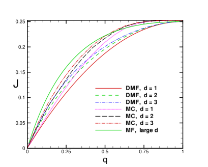
Figure 2: Fig.2: (Colour online) $J$ vs $q$ for $d=1,2,3$ obtained by DMF method and MC simulation.

II.2 Interacting Subsystem Approximation

Interacting subsystem approximation (ISA) is another method of calculating stationary properties of ASEPs with a single defect or a single bottleneck developed by Greulich and Schadschneider greulich1 . It can be easily extended to the case of asymmetric exclusion processes with 2 defects separated by $d$ lattice sites. Similarly to DMF this method divides the lattice into several segments. Particle dynamics inside the segments is treated exactly, while between the segments mean-field assumptions are made. ISA differs from DMF in the defining of segments. In DMF the position of defects separates different parts, and there is always 3 segments in the system. In ISA the sites that are connected by the defect bond are put together in one segment, as shown in Fig. 3.

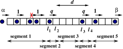
Figure 3: Fig.2: (Colour online) Fig.3: (Colour online) interacting subsystems connected via mean-field assumption. For d$>$2 the system is divided into five segments.

For $d=1$ there are also 3 parts in the lattice, and the middle segment has 3 sites. For $d=2$ there are 4 segments and 2 middle segments (with 2 lattice sites each) border each other. For any larger distance between local inhomogeneities ISA assumes 5 segments: see Fig. 3. Note that the size of the middle segment is equal to $d-2$.

Let us consider a general case of 5 segments ($d>2$) for computation of stationary properties of ASEPs with 2 defects. As was argued above, the system can be found in one of three phases: LD, HD or HD/LD (maximal-current). Since the derivation of properties in HD and LD phases is the same as for DMF approach, we concentrate on description of the maximal-current phase. As before we assume that the bulk density in the segments 1 and 5 are $1-\rho^{*}$ and $\rho^{*}$ correspondingly. Let us define $l_{1}$ and $l_{2}$ as the probabilities to find the particles at the corresponding sites of the segment around the first defect. Similarly, $l_{3}$ and $l_{4}$ describe densities in the segment around the second defect bond. For the middle segment with $d-2$ lattice sites we define $x_{i}$ for $i=1,\cdots,d-2$ as the particle density at $i$-th site of this segment. As for DMF approach, the existing particle-hole symmetry simplifies calculations significantly. Specifically, it suggests that

$$l_{4}=1-l_{1},\quad l_{3}=1-l_{2},\quad x_{i}=1-x_{d+1-i}.$$ (23)

The overall particle current in the system can be written as

$$J=\rho^{*}(1-\rho^{*}),$$ (24)

while due to the mean-field assumptions the current between the first and the second segments is equal to

$$J_{12}=(1-l_{1})(1-\rho^{*})=\alpha_{2}(1-\rho^{*}),$$ (25)

where $\alpha_{2}$ is the effective rate to enter the second segment. At large times we expect to find the system in the stationary state, i.e., $J=J_{12}$, yielding

$$1-\alpha_{2}=l_{1}=(1-\rho^{*}).$$ (26)

The current between segments 2 and 3 can be presented in the several ways,

$$J_{23}=l_{2}(1-x_{1})=\beta_{2}l_{2}=\alpha_{3}(1-x_{1}),$$ (27)

with $\beta_{2}$ being the effective exit rate from the segment 2, while $\alpha_{3}$ is the effective rate to enter the segment 3. When the system reaches stationary phase, $J=J_{23}$, and we obtain

$$\beta_{2}=1-x_{1},\quad\alpha_{3}=\frac{\rho^{*}(1-\rho^{*})}{1-x_{1}}.$$ (28)

Because of the particle-hole symmetry the effective entrance and exit rates from the segment 3 are the same, $\alpha_{3}=\beta_{3}$. The particle current via the ASEP segment with $N$ sites and with entrance and exit rates $\alpha$ and $\beta$, respectively, $J(\alpha,\beta,N)$, can be calculated explicitly derrida93 . Then to obtain stationary properties of ASEP with 2 defects in the maximal-current phase the following system of equations should be solved,

$$\rho^{*}(1-\rho^{*})=qJ(\frac{1-\rho^{*}}{q},\frac{1-x_{1}}{q},2);$$

$$\rho^{*}(1-\rho^{*})=J(\frac{\rho^{*}(1-\rho^{*})}{1-x_{1}},\frac{\rho^{*}(1-\rho^{*})}{1-x_{1}},d-2).$$ (29)

where $\rho^{*}$ and $x_{1}$ are 2 unknown variables. The expression on the right side of the first equation describes the current inside the segment 2 and 4. Because the hopping rate is $q<1$, the effective entrance and exit rates must be rescaled by the same factor. The right side of the second equation gives the current inside the segment 3. The application of ISA for $d=1$ and $d=2$ cases is different. In the case of 2 consecutive defect bonds the system is divided only in 3 segments. The middle segment has 3 sites that surround defect bonds. In the HD/LD phase the effective entrance rate is $\alpha_{2}=1-\rho^{*}$, and the stationary properties can be obtained by solving only one equation

$$\rho^{*}(1-\rho^{*})=qJ(\frac{1-\rho^{*}}{q},\frac{1-x_{1}}{q},3).$$ (30)

Using Eqs. (4) and (5) for the middle segment with equal entrance and exit rates gives us

$$\rho^{*}(1-\rho^{*})=\frac{q(1-\rho^{*})\left[2(1-\rho^{*})+3q\right]}{2\left[2(1-\rho^{*})^{2}+3q(1-\rho^{*})+2q^{2}\right]},$$ (31)

which can be simplified into the following expression,

$$4(\rho^{*})^{3}-2(3q+4)(\rho^{*})^{2}+4(q+1)^{2}\rho^{*}-q(3q+2)=0.$$ (32)

This cubic equation can be solved explicitly, yielding

$$\rho^{*}=\left[3q+4+(4-3q^{2})/D+D\right]/6,$$ (33)

where

$$D=\left[-8+9q^{2}-27q^{3}+3\sqrt{3}\sqrt{16q^{3}-q^{4}-18q^{5}+28q^{6}}\right]^{1/3}.$$ (34)

ISA also works differently in the case of $d=2$. There are 4 segments in the system, and because of the neglect of correlations between segments 2 and 3 we have

$$l_{2}(1-l_{3})=l_{2}^{2}=\rho^{*}(1-\rho^{*}).$$ (35)

Then the effective entrance rate to the segment 2 is $\alpha_{2}=1-\rho^{*}$, and the effective exit rate is equal to $\beta_{2}=l_{2}=\sqrt{\rho^{*}(1-\rho^{*})}$. The unknown parameter $\rho^{*}$ is determined from the equation for the stationary current,

$$\rho^{*}(1-\rho^{*})=qJ(\frac{\alpha_{2}}{q},\frac{\beta_{2}}{q},2).$$ (36)

Substituting the values of the effective boundary rates and utilizing Eq. (12) we obtain

$$\rho^{*}\sqrt{1-\rho^{*}}+(\rho^{*})^{3/2}=q\sqrt{1-\rho^{*}}.$$ (37)

which can be recast in the form of a cubic equation:

$$2(\rho^{*})^{3}-(2q+1)(\rho^{*})^{2}+(q^{2}+2q)\rho^{*}-q^{2}=0,$$ (38)

This equation can be solved analytically but for brevity we do not write the solution. It can also be shown that in the limit of $d\gg 1$ ISA method with 2 defects produces the stationary current and bulk densities which are indistinguishable form the situation with only one defect greulich1 ,

$$\rho^{*}=\left[3q+2-\sqrt{9q^{2}-4q+4}\right]/4,$$

$$J=\left[2q-9q^{2}+3q\sqrt{9q^{2}-4q+4}\right]/8.$$ (39)

Let us now exhibit the dependence of $J$ on q in the ISA method. In figure (4) we have drawn $J$ vs $q$ for $d=1,2$ and have compared the results to those obtained by DMF method and MC simulations.

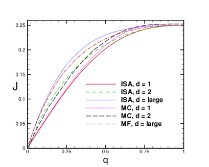
Figure 4: Fig.4: (Color online) Current vs q for $d=1,2$ and a large $d$ obtained within ISA method and MC simulation. In simulations we have taken $\alpha=\beta=0.6$.

In general, ISA method gives a better estimation of current compared to DMF at least for small values of $d$ we have considered.

III Correlations near defect

III.1 Monte Carlo Simulations

In this section we aim to investigate correlations in the vicinity of defects. We restrict ourselves to adjacent two-point correlations and will present our results for the general two-point and multi-point correlations in a future work. Let us now introduce the normalized connected two-point correlation function $C_{i}$ between the neighbouring sites $i$ and $i+1$. This quantity is defined as follows:

$$C_{i}=\frac{\langle\tau_{i}\tau_{i+1}\rangle-\langle\tau_{i}\rangle\langle\tau_{i+1}\rangle}{\sqrt{\langle\tau_{i}^{2}\rangle-\langle\tau_{i}\rangle^{2}}\sqrt{\langle\tau_{i+1}^{2}\rangle-\langle\tau_{i+1}\rangle^{2}}}~{}i=1,\cdots,L-1.$$ (40)

The function $C_{i}$ measures the correlation and it lies between $-1$ and $1$. Negative values correspond to anti-correlation between neighboring sites whereas a positive value signifies correlation. The values near zero are regarded as uncorrelated. Fig. (5) depicts the simulated profiles of correlation at $d=10$ and 100 each for three values of $q$. The system size is $L=500$ and we have taken $\alpha=\beta=0.6$ in all our simulation results unless stated otherwise. The system has been updated for $T$ Monte Carlo steps. Each step consists of $L$ moves. In each move, we randomly choose a site and update its status according to ASEP rules described above. We discard the first $\frac{T}{5}$ steps to ensure reaching steady state, and we have accumulated data separated by 10 MC steps to avoid any possible temporal correlations. The value of $T$ is taken $10^{8}$ in our simulations.

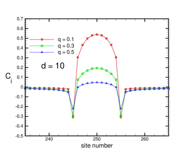
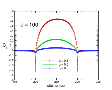
Figure 5: Fig.5: (Color online) Profile of normalized correlation function at $d=10$ (top) and $d=100$ (bottom) for $q=0.1,0.3,0.5$.

Two defects are symmetrically placed with respect to chain mid point. We observed that correlations are large in sites between the defects. There is a rather strong anti-correlation in the sites immediately after the first defect and before the second defect. The correlations are growing up for middle sites where the maximum value is achieved. It can be seen that correlations are greater when $d$ is increased. This is unexpected and counterintuitive because increasing the distance between the defects reduces their interaction. It has been observed via MC simulations that when $d$ is increased the current reaches asymptotically to its mean-field value $J_{MF}=\frac{q}{(1+q)^{2}}$ dong07 ; dongPRE . Therefore, one expects the correlations to exhibit a reducing behavior with respect to distance $d$ but this is not observed in our simulations. To have a deeper understanding, we have sketched the behavior of correlation profile upon varying the distance $d$ for $q=0.1$ and $q=0.3$ in Fig. 6.

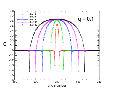
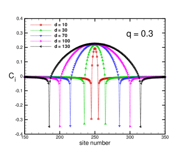
Figure 6: Fig.6: (Color online) Profile of normalized correlation functions at various values of $d$ for $q=0.1$ (top) and $q=0.3$ (bottom).

For fixed values of $q$, increasing the distance $d$ between the defects gives rise to enhancement of correlations/antocorrelations. For instance, the correlation value in the middle point rises from roughly 0.5 at small $d\sim 10$ to 0.65 for $d\sim 100$. It can be observed that there is no notable difference in correlation values for $d$ larger than $100$. Moreover, the correlations are always greater than anti-correlations. By increasing $q$, the correlations/anti-correlations are notably reduced in values. This is expected since in the limit of homogeneous ASEP where $q\rightarrow 1$ the correlation functions become very small. Here we wish to make a pause and have a discussion on correlations in normal ASEPs. In fact the middle segment between two defects can be regarded as an ASEP chain with length $d$ with equal entrance and exit rates. To the best of our knowledge, correlations in ASEP with random sequential update, has only been analytically discussed by Derrida and Evans who obtained exact analytical expression for a general two-point function and made a conjecture to generalize their findings to $n$-point function evans93 . Their study was restricted to the special case $\alpha=\beta=1$ and they found that long range correlations persist in the bulk which was attributed as a boundary effect. In order to see if the large value of the connected two-point function survives in the normal ASEP with equal entrance and exit rates, we performed MC simulations. Our results show that when $\alpha=\beta$, the profile of $C_{i}$ reaches a small constant (almost zero) in the bulk. The correlations become large near boundaries. This boundary behaviour depends on whether $\alpha=\beta<0.5$ or $\alpha=\beta>0.5$. Figure (7) illustrates this aspect.

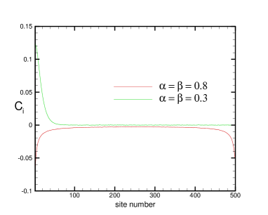
Figure 7: Fig.7: (Color online) Profile of normalized correlation functions in a normal ASEP chain with $\alpha=\beta$ .

We recall that correlations in other types of update such as parallel updating has been discussed in schutz93 ; schutz93PRE . It is worthwhile to examine the behavior of density profile between defects. Dong et al have recently shown via extensive MC simulations that the density profile takes a linear shape between defects dong07 . This behavior remains unchanged in ASEP with extended objects dongPRE . For the sake of completeness, we show some typical density profiles in Fig. 8.

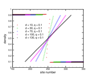
Figure 8: Fig.8: (Color online) Profile of density at various values of $d$ for $q=0.1$. The profile exhibits a linear behaviour with positive slope. This behaviour is associated to the existence of wandering shock in the region between left and right defects.

The interesting point is the absence of boundary layer in this phase-segregated regime. It would be illustrative to look at the dependence of two-point correlation functions at some particular sites on values of $q$ and $d$. These results are sketched in Fig. 9 where correlations at the first defect site ($d_{1}$), its rightmost site ($d_{1}+1$) and in the middle site of the chain are considered.

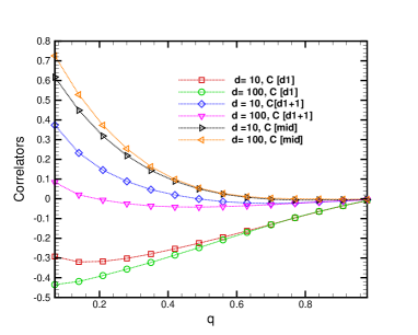
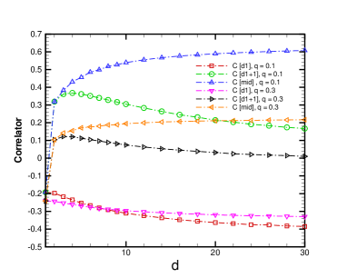
Figure 9: Fig.9: (Color online) Dependence of normalized correlation functions at three selected sites on $q$ (top) and on $d$ (bottom).

Note that all correlations/anti-correlations approach zero when $q$ tends to one. Moreover, increasing defect’s separation $d$ increases the correlations. The dependence on $d$ is more interesting. While the values of correlation functions reach an asymptotic value at large d, the behavior is not monotonous. Especially for $C_{d_{1}+1}$ correlation increases up to a maximum and then begin to decrease smoothly towards its asymptotic value. The value of $d$ where $C_{d_{1}+1}$ is maximized does not show a significant dependence on $q$. In can be concluded that varying $d$ can dramatically affect the system characteristics as far as correlations are considered.

III.2 Analytical theory

Our simulation findings in the preceding section confirms that in between the defects the correlations are notably higher than other sites. In this section we try to develop a theoretical framework to capture this feature. Suppose we have two slow defects located in the bulk at sites $k$ and $l$ ($k<l$) respectively both with rate $q$. The mean occupation at site $i$ in the steady state is denoted by $n_{i}=\langle\tau_{i}\rangle$, in which $\tau_{i}=0,1$ is the occupation number at site $i$. We assume that a simple MF assumption, i.e., $\langle\tau_{i}\tau_{i+1}\rangle=\langle\tau_{i}\rangle\langle\tau_{i+1}\rangle=n_{i}n_{i+1}$ holds for all sites except $i=k,\cdots,l$ i.e.; defective sites themselves and all the sites between them. At these sites the correlations are strong enough to violate the simple mean-field assumption. Let us introduce two-point correlation functions $m_{i}$ in the following way,

$$m_{i}=\langle\tau_{i}\tau_{i+1}\rangle.$$ (41)

There are $L+l-k+2$ unknowns, namely, $n_{1},n_{2},\cdots,n_{L},m_{k},m_{k+1},\cdots,m_{l}$ and lastly the current $J$. In the stationary state there exists $L+1$ equations among these unknowns. Let us label them by $A_{0}$ to $A_{L}$. These equations can be obtained by expressing the current $J$ in terms of the mean site densities and two point correlators. The first equation, $A_{0}$, is $J=\alpha(1-n_{1})$. The equations $A_{i}$ for $~{}i=1,\cdots,k-1$ and $i=l+1,\cdots,L-1$ have the following form,

$$J=n_{i}(1-n_{i+1}).$$ (42)

Equation $A_{k}$ is:

$$J=q\langle\tau_{k}(1-\tau_{k+1})\rangle=q(n_{k}-m_{k}).$$ (43)

Similarly, equation $A_{l}$ is given below

$$J=q\langle\tau_{l}(1-\tau_{l+1})\rangle=q(n_{l}-m_{l}).$$ (44)

Equations $A_{i}~{}(i=k+1,\cdots,l-1)$ have the following form

$$J=\langle\tau_{i}(1-\tau_{i+1})\rangle=(n_{i}-m_{i+1}).$$ (45)

lastly equation $A_{L}$ is as follows,

$$J=\beta\langle\tau_{L}\rangle=\beta n_{L}.$$ (46)

We do not intend to add more equations. Unfortunately the above equations are nonlinear and it would be a formidable task to solve them analytically. Alternatively, we shall utilize a numerical approach to solve the system of equations by exploiting their recursive structure. This approach was originally introduced in foulaadvand07 in the context of disordered ASEP and was later applied to the problem of two intersecting ASEP chains foulad07 . According to this numerical scheme, we assign a value to $J$. Having $J$, it is possible to iterate equations (in forward direction) and obtain $n_{1}$ up to $n_{k}$. Then we proceed to find $m_{k}$ by incorporating the relation $J=q(n_{k}-m_{k})$. At this stage it is not possible to proceed further because both $n_{k+1}$ and $m_{k+1}$ are unknown and we have only one relation between them : $J=n_{k+1}-m_{k+1}$. In order to proceed, we approximate $n_{k+1}$ in the following way. Consider the rate equation for the 2-point function $\langle\tau_{k}\tau_{k+1}\rangle$ which is governed by the following master equation:

$$\frac{d\langle\tau_{k}\tau_{k+1}\rangle}{dt}=\langle\tau_{k-1}(1-\tau_{k})\tau_{k+1}\rangle-\langle\tau_{k}\tau_{k+1}(1-\tau_{k+2})\rangle.$$ (47)

In the steady state, the left hand side becomes zero, and therefore two terms on the right hand side will be equal. To proceed further we have to approximate 3-point functions. This is achieved by utilizing the cluster mean-field assumption chowdhury02 . According to this assumption we replace any three point function by the product of 2-point functions as follows,

$$\langle n_{i}n_{j}n_{k}\rangle=\frac{\langle n_{i}n_{j}\rangle\langle n_{j}n_{k}\rangle}{\langle n_{j}\rangle}.$$ (48)

We then replace all 2-point functions by the product of 1-point functions except $m_{k}=\langle\tau_{k}\tau_{k+1}\rangle$. Then it is possible to express $1-n_{k+2}$ in terms of $n_{k-1},m_{1}$ and $n_{k+1}$. After some algebra a quadratic equation for $n_{k+1}$ is obtained:

$$n_{k-1}n_{k+1}^{2}-m_{k}n_{k-1}n_{k+1}-m_{k}J=0.$$ (49)

The physically reasonable solution for this equation is given by

$$n_{k+1}=\frac{m_{k}+\sqrt{m_{k}^{2}+\frac{4m_{k}J}{n_{k-1}}}}{2}.$$ (50)

Now it is possible to find $m_{k+1}$ via equation $J=n_{k+1}-m_{k+1}$. Analogous to the above procedure we can find $n_{k+2}$ as follows:

$$n_{k+2}=\frac{qm_{k}m_{k+1}+\sqrt{(qm_{k}m_{k+1})^{2}+4qJn_{k}n_{k+1}^{2}m_{k+1}}}{2qn_{k}n_{k+1}}.$$ (51)

After having $n_{k+2}$ we simply obtain $m_{k+2}$ via equation $J=n_{k+2}-m_{k+2}$. Now it would be possible to proceed iteratively after taking into account some approximation. To this end we recall the equality

$$\frac{d\langle\tau_{i}\tau_{i+1}\rangle}{dt}=\langle\tau_{i-1}(1-\tau_{i})\tau_{i+1}\rangle-\langle\tau_{i}\tau_{i+1}(1-\tau_{i+2})\rangle.$$ (52)

Putting the left hand side equal to zero in the steady state, utilizing cluster mean-field in three point functions and finally substituting $m_{i+1}$ by $m_{i+1}=n_{i+1}-J$ we arrive at the following equation:

$$n_{i+1}=\frac{m_{i-1}m_{i}+\sqrt{(m_{i-1}m_{i})^{2}+4Jn_{i-1}n_{i}^{2}m_{i}}}{2n_{i-1}n_{i}}.$$ (53)

Note that we have approximated $\langle\tau_{i-1}\tau_{i+1}\rangle$ by the mean-field relation $\langle\tau_{i-1}\rangle\langle\tau_{i+1}\rangle$. We can iterate equation (53) together with $m_{i+1}=n_{i+1}-J$ from $i=k+2$ to $l-2$ to find the corresponding $n_{i}$ and $m_{i}$ up to $i=l-1$. The site $i=l$ needs to be treated separately. Following the same strategy we easily find:

$$n_{l}=\frac{m_{l-2}m_{l-1}+\sqrt{(m_{l-2}m_{l-1})^{2}+4Jn_{l-2}n_{l-1}^{2}m_{l-1}}}{2n_{l-2}n_{l-1}}.$$ (54)

From which one can compute $m_{l}$. In a similar fashion, we can obtain $n_{l+1}$. We only should shift up all the subscripts in equation (54) by one. Now it is possible again to proceed iteratively to the end of the chain and evaluate $n_{L}$ which gives us the output current $J^{out}$. If the given value of input $J$ were correct, the output current $J^{out}$, which is $\beta n_{L}$, should be the same, up to a given precision, as the input value of $J$. By systematically increasing the input $J$ in an small amount $\delta J$, we can determine the correct $J$ and correspondingly the mean densities $n_{1},\cdots,n_{L}$ together with correlators $m_{k},\cdots,m_{l}$. In Fig. (10) the dependence $J$ on $q$ obtained by the numeric scheme devised above is sketched. For the sake of comparison, we have augmented the figure with the analogous graphs obtained by MF, DMF, ISA and MC methods.

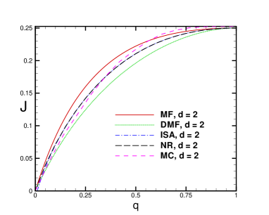
Figure 10: Fig.10: (Color online) Current vs q for $d=2$ obtained by various analytical and numerical methods and MC simulation. $J$ approaches to 0.25 when $q$ tends to one in accordance to normal ASEP.

The result of the numerical scheme is almost identical to ISA method. They both are in very good agreement with Monte Carlo simulations. However, the numerical scheme has an advantage over ISA method in the sense that it can easily be implemented for any $d$, whereas finding the solution of the ISA nonlinear set of equations, i.e., Eq. (29) is not an easy task even by employing advanced numerical methods. Finally in figure (11) we have sketched the dependence of $J$ on $d$ obtained from MC simulation and the numeric scheme.

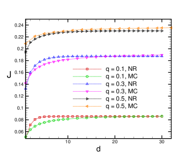
Figure 11: Fig.11: (Color online) Current vs $d$ for $q=0.1,0.3$ and $0.5$ obtained by the numeric method and MC simulation.

The results of the numeric method are in rather good agreement with those obtained by MC simulations. $J$ is an increasing function of $d$ and becomes saturated after some short $q$-dependent distance. The results confirms the earlier finding in dong07 . Note that the length scale on which $J$ recovers its single-defect value is of the same order of magnitude of the correlation length in the density profile near boundaries. Finally we would like to add that our numerical scheme is not capable of reproducing the profile of correlators obtained via MC simulations. Figure (12) depicts the profile of unnormalised adjacent two-point correlation function $\langle\tau_{i+1}\tau_{i}\rangle-\langle\tau_{i+1}\rangle\langle\tau_{i}\rangle$ for two methods of simulation and numerical scheme.

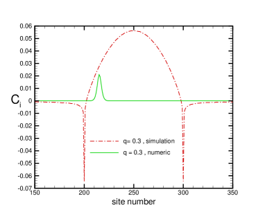
Figure 12: Fig.12: (Color online) Profile of corrrelators for $d=100$ and $q=0.3$.

We see that within the numerical framework both the value and the extension of correlators are small in comparison to the simulation results. The reason lies in the implementation of a series of approximation in several places in this numerical algorithm.

IV Summary and Conclusions

An open ASEP chain with two defective sites with reduced hopping rates $q<1$ has been investigated. The system current and mean site densities at defective sites and their vicinities have been obtained by two analytical methods namely defect mean-field (DMF) and interacting subsystem approximation (ISA). Both methods combine mean-field approach near defects with known exact solutions. Our results are accomplished by extensive Monte Carlo simulations. We focus on the phase-segregated phase in which defects globally affect the system properties and the system is not input/output rate-limited but rather defect-limited. MC simulations have revealed strong short ranged correlations at the defective sites and at all the site between them. Additionally, the profile of density between defects takes a linear form which marks the existence wandering shock in this intermediate region. In order to take into account these correlations, we have introduced a numerical approach which utilizes a cluster mean-field assumption. Comparison of the three methods show that ISA and the numeric approach give a current value which is in a good agreement with MC simulations. DMF method however, only gives a good results compared to MC and other two methods for small $q$ less than $0.1$ which is due to strong correlations. Furthermore, we have obtained the profile of neighbouring two-point correlation function throughout the chain. It is shown that these two point correlators exhibit a rather strong anti correlation at the first defective site then they grow to the middle of the defects and after that they start diminishing. In general, two point correlators will tend to a tiny value when $q$ approaches one. However, the dependence of two point correlators for a fixed $q$ as a function of distance between defects is not monotonous. Despite reaching to an asymptotic value for large distances, one observes a peak at short distances for the two point correlators near defects. Our theoretical analysis indicates that correlations are critically important for dynamics of particles in disordered ASEPs. It also shows that it is possible to devise an approximate method that can take into account these correlations, providing a satisfactory description of stationary properties.

References

- (1) B. Derrida, Phys. Rep. 301 65 (1998).
- (2) B. Schmittmann and R.K.P. Zia in: Phase transitions and Crtitical Phenomena, vol 17, ed. C. Domb and L. Lebowitz (London: Academic) 1995.
- (3) G. M. Schütz, Integrable stochastic many-body systems in Phase Transitions and Critical Phenomena edited by C. Domb and J. Lebowitz (Academic, London, 2000), Vol. 19.
- (4) D. Chowdhury, L. Santen and A. Schadschneider, Phys. Rep. 329 199 (2000).
- (5) B. Derrida, M. R. Evans, V. Hakim and V. Pasquier, J. Phys. A: Math. Gen. 26 1493 (1993).
- (6) C. T. Macdonald and J. H. Gibbs, Biopolymers 6 1 (1968).
- (7) L. B. Shaw, R. K. P. Zia and K. H. Lee, Phys. Rev. E 68 021910 (2003).
- (8) T. Chou and G. Lakatos, Phys. Rev. Let. 93 198101 (2004).
- (9) L. B. Shaw, A. B. Kolomeisky and K. H. Lee, J. Phys. A: Math. Gen. 37 2105 (2004).
- (10) J. J. Dong, B. Schmittmann and R. K. P. Zia, J. Stat. Phys. 128 21 (2007).
- (11) R. Lipowsky, S. Klumpp and T. M. Nienwenhuizen, Phys. Rev. Lett. 87 108101 (2001).
- (12) A. Parmeggiani, T. Franosch and E. Frey, Phys. Rev. Lett. 90 086601 (2003).
- (13) R. A. Blythe and M. R. Evans, J. Phys. A: Math. Theor. 40 R333 (2007).
- (14) A.B.Kolomeisky, G.M.Schütz, E.B.Kolomeisky, and J.P.Straley, J. Phys. A: Math. Gen. 31 6911 (1998).
- (15) S. A. Janowsky and J. L. Lebowitz, Phys. Rev. A 45 618 (1992).
- (16) G.M. Schütz, J. Stat. Phys. 71, 471 (1993).
- (17) G.M. Schütz, Phys. Rev. E 47, 4265 (1993).
- (18) S. A. Janowsky and J. L. Lebowitz, J. Stat. Phys. 77 35 (1994).
- (19) A. B. Kolomeisky, J. Phys. A: Math. Gen. 31 1153 (1998).
- (20) G. Tripathy and M. Barma, Phys. Rev. Lett. 78 3039 (1997).
- (21) G. Tripathy and M. Barma, Phys. Rev. E 58 1911, 1998.
- (22) K. M. Kolwanker and A. Punnoose, Phys. Rev. E 61 2453, 2000.
- (23) M. Ha, J. Timonen and M. den Nijs, Phys. Rev. E 68 056122, 2003.
- (24) R. J. Harris and R. B. Stinchcombe, Phys. Rev. E 70 016108, 2004.
- (25) C. Enaud and B. Derrida, Europhys. Lett. 66 83, 2004.
- (26) R. Juhasz, L. Santen and F. Igl´i, Phys. Rev. Lett. 94 010601, 2005.
- (27) M. Barma, Physica A 372 22, 2006.
- (28) P.Pierobon, M. Mobilia, R. Kouyos and E. Frey, Phys. Rev. E, 74 031906, 2006.
- (29) M. E. Foulaadvand, S. Chaaboki and M. Saalehi, Phys. Rev. E 75 011127 (2007).
- (30) M. E. Foulaadvand and M. Neek Amal, Europhys. Lett. 80 60002, (2007).
- (31) J.J. Dong, B. Schmittmann and R.K.P. Zia, Phys. Rev. E 76 051113, 2007.
- (32) P. Greulich and A. Schadschneider, Physica A 387 1972 (2008).
- (33) P. Greulich and A. Schadschneider, J. Stat. Mech. P04009 (2008).
- (34) B. Derrida, S.A. Janowsky, J.L. Lebowitz and E.R. Speer, J. Stat. Phys. 73 813 (1993).
- (35) K. Mallick, J. Phys. A: Math. Gen 29 5375 (1996).
- (36) M.R. Evans, J. Phys. A: Math. Gen 30 5669 (1997).
- (37) H.-W. Lee, V. Popkov and D. Kim, J. Phys. A: Math. Gen 30 8497 (1997).
- (38) M.E. Fouladvand and H.-W. Lee, Phys. Rev. E, 60 6465-6479 (1999).
- (39) B. Derrida and M.R. Evans, J. Phys. I France, 3, 311 (1993).
- (40) D. Chowdhury and J.S. Wang, Phys. Rev. E 65 04126, 2002.