Detecting relic gravitational waves in the CMB: Comparison of different methods

Abstract

In this paper, we discuss the constraint on the relic gravitational waves by both temperature and polarization anisotropies power spectra of cosmic microwave background radiation. Taking into account the instrumental noises of Planck satellite, we calculate the signal-to-noise ratio $S/N$ by the simulation and the analytic approximation methods. We find that, comparing with the $BB$ channel, the value of $S/N$ is much improved in the case where all the power spectra, $TT$, $TE$, $EE$ and $BB$, are considered. If the noise power spectra of Planck satellite increase for some reasons, the value of $S/N$ in $BB$ channel is much reduced. However, in the latter case where all the power spectra of cosmic microwave background radiation are considered, the value of $S/N$ is less influenced. We also find that the free parameters $A_{s}$, $n_{s}$ and $n_{t}$ have little influence on the value of $S/N$ in both cases.

I Introduction

A stochastic background of the relic gravitational waves (RGWs), generated during the very early stage of the Universe a1 , is a necessity dictated by general relativity and quantum mechanics grishchuk0707 . The RGWs have a wide range spreading spectra grishchuk1 ; zhang1 ; others , and their detection plays a double role in relativity and cosmology.

One of the important methods for the detection of RGWs is by the cosmic microwave background (CMB) power spectra, including the temperature anisotropies ($TT$) power spectrum, the polarization ($EE$ and $BB$) power spectra, and the cross-correlation ($TE$) power spectrum a8 ; grishchuk-cmb ; a11 ; a12 ; a13 . By observing the lower-order CMB multipoles, one can detect the signal of RGWs at the very low frequencies ($10^{-17}\sim 10^{-15}$ Hz). One has to note, besides the gravitational waves of quantum-mechanical origin grishchuk0707 , the classical gravitational waves were generated at later stages of cosmological evolution othersource . However, their wavelengths are much shorter than the present Hubble radius and therefore they do not affect the lower-order CMB multipoles.

As well known, the CMB has certain degree of polarization generated via Thompson scattering during the decoupling in the early Universe a5 . In particular, if the RGWs are present at the photon decoupling in the Universe, the magnetic type of polarization ($B$-polarization) will be produced a8 ; a11 ; a12 . This would be a characteristic feature of RGWs on very large scale, since the density perturbations will not generate this polarization. So a natural way for the detection of RGWs is by observing the signal of $B$-polarization of CMB. This is the so-called “BB” method. However, the amplitude of the $B$-polarization is expected to be very small. In addition, the $B$-polarization is prone to degradation by various systematic effects on a wide range of scales wuran1 ; wuran2 ; wuran3 ; wuran4 . The current 5-year Wilkinson Microwave Anisotropy Probe (WMAP5) observation only gives an upper limit $\ell(\ell+1)C_{\ell=2-6}^{BB}/2\pi<0.15\mu$K² ($95\%$C.L.)5map . The forthcoming projects, such as the Planck Planck , Clover clover , Spider spider , QUITE quiet , are expected to be much more sensitive for the detection of the CMB $B$-polarization.

Due to the disadvantage of “BB” method, it is necessary to look for the new method for the detection of RGWs in the CMB. In the previous work a12 , the authors found that, in the large scale $(\ell<50)$, the RGWs generate the negative $TE$ spectrum. However, if the $TE$ spectrum is generated by density perturbations, it should be positive. This suggests that the signal of RGWs can also be detected by the CMB $TE$ spectrum. Comparing with the $B$-polarization, the amplitude of the $TE$ spectrum is nearly two order larger. In the works polnarev ; ours , the authors have developed several ways to detect the signal of RGWs directly from the CMB $TE$ spectrum. These are the so-called “TE” method.

In the work ours we found the WMAP5 $TE$ data contains a hint of the presence of RGWs contribution. In terms of quadrupole ratio $R$, the best-fit model produced $R=0.24$, which corresponds to the tensor-to-scalar ratio $r\simeq 0.48$. Because of large residual noise, the uncertainty of this determination is still large. We also found, if considering the Planck instrumental noises, “TE” method can detect the signal of RGWs at 2$\sigma$ level when $r>0.3$. If considering the ideal case with full sky and no noise, “TE” method can detect the RGWs at 2$\sigma$ level when $r>0.1$. By comparing the detection abilities of “TE” and “BB” methods, we found that, taking into account of the instrumental noises of Planck satellite, “BB” method is more sensitive when $r$ is small. However, if the noise power spectra or the amplitudes of RGWs increase, the sensitivity of “TE” method becomes better than that of “BB” method.

In this paper, we shall extend the “TE” method in our previous work ours . By calculating the values of $S/N$, we shall compare the detection abilities for the RGWs in the following four cases. The first case (“B” case) is the so-called “BB” method, where only the $B$-polarization spectrum is considered. In the second case, we include not only the CMB $TE$ spectrum, but also the $TT$ spectrum. We call it as the “CT” case (“C” standing for the cross-correlation power spectrum and “T” standing for the temperature anisotropies power spectrum). We shall expect that, taking into account the contribution of $TT$ spectrum, the detection ability will be much improved. In the third case, besides $TE$ and $TT$ spectra, we also include the $EE$ spectrum. We call it as the “CTE” case. The fourth one is the “CTEB” case, where the contributions of $TE$, $TT$, $EE$ and $BB$ power spectra are all considered. The detection ability in this case is expected to be much more sensitive than the other three cases.

The organization of this paper is as follows. In Section II, the primordial power spectra of RGWs and density perturbations, the CMB power spectra and the corresponding estimators are introduced. In this section, the probability density functions (pdfs) for the estimators are also discussed. In Section III, we introduce four (“B”, ‘CT”, “CTE” and “CTEB”) cases for the detection of RGWs in the CMB. The likelihood functions are also given this section. In Section IV, by constructing the likelihood functions based on the simulated data, we shall investigate the values of the signal-to-noise ratio $S/N$ in these four cases. This quantity describes the detection abilities of RGWs in the different cases. We firstly introduce the simulation method. In the simulation, when constructing the likelihood functions, we only consider one free cosmic parameter, the tensor-to-scalar ratio $r$. We find when $r>0.06$ ($r>0.16$, $r>0.13$, $r>0.05$), the signal of RGWs can be detected in “B” (“CT”, “CTE”, “CTEB”) case at $2\sigma$ level. In Section V, we discuss the analytic approximation of the likelihood functions. By the analytic approximation formulae, we obtain a simple analytic form of $S/N$, which clearly shows the dependence of $S/N$ on the amplitude of RGWs and the noises. By analyzing the analytic form of $S/N$, we find that, in “CT” and “CTE” cases, the main contributions come from the data in the intermedial scale $10<\ell<70$. However, in “B” case, the main contribution comes from the data in the very large scale $\ell<10$. In Section VI, by the simulation method, we find that, the free parameters (the tensor spectral index $n_{t}$, the amplitude of scalar spectrum $A_{s}$ and the scalar spectral index $n_{s}$) have little influence on the determination of RGWs. Section VII is the conclusion that summarizes the main results of this paper.

II Gravitational field perturbations, CMB power spectra and their estimators

II.1 Primordial power spectra of the gravitational field perturbations

The CMB temperature and polarization anisotropies power spectra are determined by the primordial power spectra of density perturbations (scalar perturbations) and RGWs (tensor perturbations), and the time evolution of these perturbations during and after the epoch of recombination. Before proceeding with the CMB power spectra, it is necessary to introduce the primordial perturbation spectra, which are usually assumed to be power-law. This form is a generic prediction of a wide range of scenarios of the early universe a1 ; a4 ; grishchuk1 . In general there might be deviations from a power-law, parametrized in terms of the running of the spectral index (see for example liddle ), but we shall not consider this probability in the current paper. Thus the primordial power spectra of the perturbation fields have the forms

$$\begin{array}[]{c}P_{s}(k)=A_{s}(k_{0})\left(\frac{k}{k_{0}}\right)^{n_{s}-1},~{}~{}~{}P_{t}(k)=A_{t}(k_{0})\left(\frac{k}{k_{0}}\right)^{n_{t}},\end{array}$$ (2)

where $n_{s}$ and $n_{t}$ are the scalar and tensor spectral indices, respectively. $k_{0}$ is pivot wavenumber, which can be arbitrarily chosen. In the WMAP paper peiris , the pivot wavenumber $k_{0}=0.002$Mpc^-1 is used, which is close to the observable horizon. The scale $k_{0}=0.05$Mpc^-1 is also commonly used, being the default scale of CAMB package cosmomc . A number of authors have suggested other pivot wavenumber $k_{0}$ for different reasons pivot1 . In Eq. (2), $A_{s}(k_{0})$ and $A_{t}(k_{0})$ are the amplitudes of the primordial scalar and tensor spectra respectively, at the pivot scale $k_{0}$.

We can re-parameterize the tensor power spectrum amplitude $A_{t}(k_{0})$ by the “tensor-to-scalar ratio” $r$, which is defined by

$$r(k_{0})\equiv\frac{A_{t}(k_{0})}{A_{s}(k_{0})}.$$ (3)

In addition, the ratio of tensor quadrupole to scalar quadrupole $R$ is also quoted when referring to the tensor-to-scalar ratio (see for instant knox ; ours ). The relation between $R$ and $r$ is somewhat cosmology-dependence, especially on the dark energy density $\Omega_{\Lambda}$. The conversion is $R\simeq\frac{0.84-0.025\Omega_{\Lambda}-0.084\Omega_{\Lambda}^{2}}{1.04-0.82\Omega_{\Lambda}+2\Omega_{\Lambda}^{2}}r$ R_r . For the cosmological models with $\Omega_{\Lambda}=0.76$, these two definitions are simply related by $r\simeq 2R$. In the previous work ours , we have adopted $R$. However, in this paper we shall use $r$, the default quantity used in the CAMB package camb .

Using Eqs. (2) and (3), one can evaluate $r$ at a different wavenumber $k_{1}$,

$$r(k_{1})=r(k_{0})\left(\frac{k_{1}}{k_{0}}\right)^{n_{t}-n_{s}+1}.$$ (4)

In the following discussion, we shall discuss the constraint on the parameter $r$ by the simulated data. From the relation (4) we find that, if the spectral indices $n_{t}$ and $n_{s}$ are fixed as $n_{t}=0$ and $n_{s}=1$ in the likelihood analysis (the case in Sections IV and V), we have $r(k_{1})\equiv r(k_{0})$, the tensor-to-scalar ratio $r$ has the exactly same value at all pivot wavenumbers. So we do not need to differentiate the tensor-to-scalar ratio at the different pivot scales. However, if the spectral indices are free parameters in the likelihood analysis (the case in Section VI), comparing with $r(k_{0})$, the constraint of $r(k_{1})$ is also influenced by the spectral indices. So in this case, we should differentiate the tensor-to-scalar ratio at the different pivot wavenumbers. This effect will be clearly shown in Section VI.

We should mention that, in the specific early universe models, the parameters $A_{s}$, $n_{s}$, $r$ and $n_{t}$ are always not separate relation . However, in this paper we shall avoid any specific model, and consider the parameters $A_{s}$, $n_{s}$, $r$ and $n_{t}$ as the independent parameters in the data analysis.

II.2 CMB power spectra

The CMB radiation field is usually characterized by four Stokes parameters ($I,Q,U,V$). $I$ is the total intensity of radiation, $Q$ and $U$ describe the magnitude and direction of linear polarization, and $V$ is the circular polarization. From these Stokes parameters, we can construct four invariant quantities ($I,V,E,B$), which can be expanded over ordinary spherical harmonics (see a12 for details). The set of multipole coefficients $(a_{{\ell}m}^{T},a_{{\ell}m}^{V},a_{{\ell}m}^{E},a_{{\ell}m}^{B})$ completely characterize the intensity and polarization of the radiation field. Since Thompson scattering of initial unpolarized light cannot generate circular polarization, we shall not consider the $V$ stokes parameter in the following discussion.

In general, the output of the CMB experiment $a_{\ell m}^{X}$ ($X=T,E,B$), consists of two contributions, the signal convolved with the beam window function $a_{\ell m}^{X}(s)W_{\ell}$ and the noise $a_{\ell m}^{X}(n)$, i.e.

$$a_{\ell m}^{X}=a_{\ell m}^{X}(s)W_{\ell}+a_{\ell m}^{X}(n).$$ (5)

We shall use the notations $(s)$ and $(n)$ to denote the signal and noise. These two contributions are uncorrelated to each other.

Assuming the primordial perturbation fields (including the scalar perturbations and tensor perturbations) are Gaussian fields, which induces that the signal term $a_{\ell m}^{X}(s)$ has the covariance ours

$$\frac{1}{2}\langle a_{\ell m}^{X}(s)a_{\ell^{\prime}m^{\prime}}^{X^{\prime}*}(s)+a_{\ell m}^{X*}(s)a_{\ell^{\prime}m^{\prime}}^{X^{\prime}}(s)\rangle=C_{\ell}^{XX^{\prime}}\delta_{\ell\ell^{\prime}}\delta_{mm^{\prime}},$$ (6)

where $C_{\ell}^{XX^{\prime}}$ is known as the CMB power spectra, which depends on the cosmological inputs. When $X=X^{\prime}$, $C_{\ell}^{XX^{\prime}}$ is the auto-correlation power spectra, and when $X\neq X^{\prime}$, $C_{\ell}^{XX^{\prime}}$ is the cross-correlation power spectra. In absence of any parity-violating processes, the only survived cross-correlation power spectra is $C_{\ell}^{TE}$ lue . So the temperature and polarization anisotropies can be described completely by four power spectra: $C_{\ell}^{TT}$, $C_{\ell}^{EE}$, $C_{\ell}^{BB}$ and $C_{\ell}^{TE}$.

The noise terms $a_{\ell m}^{X}(n)$ and the window function $W_{\ell}$ depend on the experiment. We assume the noise is a spatially uniform Gaussian white noise. For an experiment with some known beam width and sensitivity, the noise power spectra and window function can be approximated as

$$N_{\ell}^{XX^{\prime}}=\frac{1}{2}\langle a_{\ell m}^{X}(n)a_{\ell^{\prime}m^{\prime}}^{X^{\prime}*}(n)+a_{\ell m}^{X*}(n)a_{\ell^{\prime}m^{\prime}}^{X^{\prime}}(n)\rangle=(\theta_{\rm FWHM}\sigma_{X})^{2}\delta_{XX^{\prime}}\delta_{\ell\ell^{\prime}}\delta_{mm^{\prime}},$$ (7a)

$$W_{\ell}=\exp\left[-\frac{\ell(\ell+1)}{2}\frac{\theta^{2}_{\rm FWHM}}{8\ln 2}\right],$$ (7b)

where $$\theta_{\rm FWHM} \sigma_{X} X\neq X^{\prime} \ell$$ is the full width at half maximum of the Gaussian beam, and is the root mean square of the instrumental noise. Non-diagonal noise terms (i.e., ) are expected to vanish since the noises contributions from different maps are uncorrelated. The assumption of a spatially uniform Gaussian noises spectrum ensures that the noise term is diagonal in the basis. In this paper, we shall consider the Planck instrumental noises. There are several frequency channels for the detection of CMB in Planck satellite Planck . In this paper, in order to estimate the Planck noises, we only adopt the frequency channel at 143GHz, which has the low foreground levels and the lowest noises power spectra. In this channel, we have Planck ,

$$\theta_{\rm FWHM}=7.1^{\prime},~{}~{}\sigma_{T}=6.0{\rm\mu K},~{}~{}\sigma_{E}=\sigma_{B}=11.5{\rm\mu K}.$$ (7c)

Inserting these into Eq. (7a), we obtain the noise power spectra

$$N_{\ell}^{TT}=1.53\times 10^{-4}{\rm\mu K}^{2},~{}~{}N_{\ell}^{EE}=N_{\ell}^{BB}=5.58\times 10^{-4}{\rm\mu K}^{2},~{}~{}N_{\ell}^{TE}=0.$$ (7d)

Considering Eqs. (5), (6) and (7a), we obtain the covariances of the terms $a_{\ell m}^{X}$, which are

$$\frac{1}{2}\langle a_{\ell m}^{X}a_{\ell^{\prime}m^{\prime}}^{X^{\prime}*}+a_{\ell m}^{X*}a_{\ell^{\prime}m^{\prime}}^{X^{\prime}}\rangle=(C_{\ell}^{XX^{\prime}}W_{\ell}^{2}+N_{\ell}^{XX^{\prime}})\delta_{\ell\ell^{\prime}}\delta_{mm^{\prime}}.$$ (8)

II.3 Estimators of the CMB power spectra

In Section II.2, we have introduced the CMB power spectra, which are defined as ensemble averages over all possible realization of the CMB field. However, in CMB observations, we only have access to one single realization of this ensemble. In order to obtain information on the power spectra from a single realization, it is desirable to introduce the estimators of the power spectra, which are observable quantities.

In the full sky case, and taking into account the noises, the best unbiased estimators $D_{\ell}^{XX^{\prime}}$ for the CMB power spectra $C_{\ell}^{XX^{\prime}}$ are defined by grishchuk ; ours

$$D_{\ell}^{XX^{\prime}}=\left(\frac{1}{n}\sum_{m=-\ell}^{\ell}(a_{\ell m}^{X}a_{\ell m}^{X^{\prime}*}+a_{\ell m}^{X*}a_{\ell m}^{X^{\prime}})-N_{\ell}^{XX^{\prime}}\right)W_{\ell}^{-2}~{},$$ (9)

where $n$ is the number of the degree of freedom for a fix multipole $\ell$. In the full sky case, we have $n=(2\ell+1)$. The expectation values and the standard deviations of these estimators are ours

$$\begin{array}[]{c}\langle D_{\ell}^{XX^{\prime}}\rangle=C_{\ell}^{XX^{\prime}},\\ \Delta D_{\ell}^{XX^{\prime}}=\par\sqrt{\frac{(C_{\ell}^{XX}+N_{\ell}^{XX}W_{\ell}^{-2})(C_{\ell}^{X^{\prime}X^{\prime}}+N_{\ell}^{X^{\prime}X^{\prime}}W_{\ell}^{-2})+(C_{\ell}^{XX^{\prime}}+N_{\ell}^{XX^{\prime}}W_{\ell}^{-2})^{2}}{n}}.\end{array}$$ (12)

It is necessary to investigate the pdfs for $D_{\ell}^{XX^{\prime}}$, which have been derived in ours , based on the assumption: the primordial perturbation fields and noise fields are independent Gaussian fields. In this subsection, we shall briefly introduce the results as follows (the similar results are also obtained in the Refs. wishart2 ; pdf1 ).

The pdf of the auto-correlation estimator $D_{\ell}^{XX}$ is known as the $\chi^{2}$ distribution, which is

$$f(D_{\ell}^{XX})=\frac{(nW^{2}_{\ell})V^{(n-2)/2}e^{-V/2}}{2^{n/2}\Gamma(n/2)(C_{\ell}^{XX}W_{\ell}^{2}+N_{\ell}^{XX})},$$ (13)

where $n=(2\ell+1)$ is the degree of freedom for the multipole $\ell$ in the full sky case. The quantity $V$ is defined by $V\equiv n(D_{\ell}^{XX}W_{\ell}^{2}+N_{\ell}^{XX})/(C_{\ell}^{XX}W_{\ell}^{2}+N_{\ell}^{XX})$.

The joint pdf for the estimators $D_{\ell}^{TE}$, $D_{\ell}^{TT}$ and $D_{\ell}^{EE}$ is the following Wishart distribution

$$\begin{array}[]{c}f(D_{\ell}^{TE},D_{\ell}^{TT},D_{\ell}^{EE})=\left\{\frac{1}{4(1-{\rho_{\ell}^{2}})({\sigma_{\ell}^{T}}{\sigma_{\ell}^{E}})^{2}}\right\}^{n/2}\frac{(nW_{\ell}^{2})^{3}({x}{y}-{z}^{2})^{(n-3)/2}}{\pi^{1/2}\Gamma(n/2)\Gamma((n-1)/2)}\\ \times\exp\left\{-\frac{1}{2(1-{\rho_{\ell}^{2}})}\left(\frac{{x}}{(\sigma_{\ell}^{T})^{2}}+\frac{{y}}{(\sigma_{\ell}^{E})^{2}}-\frac{2{\rho_{l}}{z}}{{\sigma_{\ell}^{T}}{\sigma_{\ell}^{E}}}\right)\right\},\end{array}$$ (16)

where the quantities $x,y,z$ are defined by: ${x}\equiv n(D_{\ell}^{TT}W_{\ell}^{2}+N_{\ell}^{TT})$, ${y}\equiv n(D_{\ell}^{EE}W_{\ell}^{2}+N_{\ell}^{EE})$, ${z}\equiv nD_{\ell}^{TE}W_{\ell}^{2}$. ${\sigma_{\ell}^{T}}=\sqrt{C_{\ell}^{TT}W_{\ell}^{2}+N_{\ell}^{TT}}$, $\sigma_{\ell}^{E}=\sqrt{C_{\ell}^{EE}W_{\ell}^{2}+N_{\ell}^{EE}}$ are the standard deviations of the multipole coefficients $a_{\ell m}^{T}$ and $a_{\ell m}^{E}$, respectively. $\rho_{\ell}$ is the correlation coefficient of $a_{\ell m}^{T}$ and $a_{\ell m}^{E}$, which can be written as,

$${\rho_{\ell}}=\frac{C_{\ell}^{TE}}{\sqrt{(C_{\ell}^{TT}+N_{\ell}^{TT}W_{\ell}^{-2})(C_{\ell}^{EE}+N_{\ell}^{EE}W_{\ell}^{-2})}}.$$ (17)

From the Wishart distribution (16), we can derive the joint pdf of the estimators $D_{\ell}^{TE}$ and $D_{\ell}^{TT}$ by integrating the variable $D_{\ell}^{EE}$, the finial result is

$$\begin{array}[]{c}f(D_{\ell}^{TE},D_{\ell}^{TT})=(nW_{\ell}^{2})^{2}{x}^{\frac{n-3}{2}}\left\{2^{1+n}\pi\Gamma^{2}(\frac{n}{2})(1-\rho_{\ell}^{2})(\sigma_{\ell}^{T})^{2n}(\sigma_{\ell}^{E})^{2}\right\}^{-\frac{1}{2}}\\ \times\exp\left\{\frac{1}{1-\rho^{2}_{\ell}}\left(\frac{{\rho_{\ell}}{z}}{{\sigma_{\ell}^{T}}{\sigma_{\ell}^{E}}}-\frac{{z}^{2}}{2x{(\sigma_{\ell}^{E})^{2}}}-\frac{{x}}{2{(\sigma_{\ell}^{T})^{2}}}\right)\right\}.\end{array}$$ (20)

We can also obtain the joint pdf for all the four estimators: $D_{\ell}^{TE}$, $D_{\ell}^{TT}$, $D_{\ell}^{EE}$, $D_{\ell}^{BB}$. Since $B$-polarization estimator $D_{\ell}^{BB}$ is independent of the estimators $D_{\ell}^{TE}$, $D_{\ell}^{TT}$ and $D_{\ell}^{EE}$, the total joint pdf is the product of the Wishart distribution $f(D_{\ell}^{TE},D_{\ell}^{TT},D_{\ell}^{EE})$ in (16) and the $\chi^{2}$ distribution $f(D_{\ell}^{BB})$ in (13) with $XX=BB$, i.e.

$$f(D_{\ell}^{TE},D_{\ell}^{TT},D_{\ell}^{EE},D_{\ell}^{BB})=f(D_{\ell}^{TE},D_{\ell}^{TT},D_{\ell}^{EE})f(D_{\ell}^{BB}).$$ (21)

We should notice that, the above results are all based on the assumption of full sky coverage. However, real experiments can only see a fraction of sky. Even for satellite experiments, a map cut must be performed in order to eliminate point sources and galactic plane foreground contaminations. As a result, different multipole moments ${a_{\ell m}^{X}}$ become correlated with each other cut1 ; wuran2 . The exact pdfs of the estimators in this case takes a rather complicated form, depending on the shape of remaining observed portion of sky wishart2 . However, for experiments probing almost the full sky (e.g. COBE, WMAP, or Planck), correlations are expected only between neighboring multipoles. In order to simplify the problem, one can take ${a_{\ell m}^{X}}$’s to be uncorrelated, and introduce a factor $f_{\rm sky}$, which denotes the observed fraction of sky. As was shown in ours ; cutpdf , for the estimators with the multipole number $\ell$, the number of degree of freedom reduces to $n_{\rm eff}=(2\ell+1)f_{\rm sky}$ (instead of $n=2\ell+1$). Thus, compared to the full sky, the inclusion of cut sky reduces the degree of freedom in the definition of the estimators $D_{\ell}^{XX^{\prime}}$. In this work, we shall discuss the CMB field with the cut sky factor

$$f_{\rm sky}=0.65,$$ (22)

which is suggested by Planck bluebook Planck . In all the following discussion, we should remember to replace $n$ with the effective degree of freedom $n_{\rm eff}$, when using the result in (12) and the pdfs in (13), (16), (20) or (21).

III Four cases to detect RGWs in the CMB

In this paper, we shall investigate the detection abilities for the RGWs in the following four cases: “B” case, “CT” case, “CTE” case and “CTEB” case, which will be introduced separately in this section.

III.1 “B” case

The first case is the well-known “BB” method. In this case, one can detect the signal of RGWs only by the observable $D_{\ell}^{BB}$, which satisfies the $\chi^{2}$ distribution in Eq. (13).

In order to study the determination of cosmic parameters from the observed data, we shall consider the likelihood function. The likelihood is a term, customarily, used to call the probability density function considered a function of an unknown parameter. Up to a constant, independent of its arguments, the likelihood is defined as the pdf of the set of the moments $D_{\ell}^{BB}$ given $C_{\ell}^{BB}$, i.e.

$$\mathcal{L}_{\rm B}\propto\prod_{\ell}f(D_{\ell}^{BB}).$$ (23)

Using the pdf in (13), and considering the effective degree of freedom $n_{\rm eff}=(2\ell+1)f_{\rm sky}$ in the cut sky, the likelihood function in (23) can be rewritten as

$$-2\ln\mathcal{L}_{\rm B}=\sum_{\ell}n_{\rm eff}\left\{\left(\frac{D_{\ell}^{BB}+N_{\ell}^{BB}W_{\ell}^{-2}}{(\sigma_{\ell}^{B})^{2}}\right)-\ln\left(\frac{D_{\ell}^{BB}+N_{\ell}^{BB}W_{\ell}^{-2}}{(\sigma_{\ell}^{B})^{2}}\right)\right\}+C_{1},$$ (24)

where $C_{1}$ is the constant for the normalization. The noise power spectrum $N_{\ell}^{BB}$ for Planck mission is given by Eq. (7d).

Since the $B$-polarization can only be generated by the gravitational waves, the observable $B$-polarization power spectrum includes a clean information of the gravitational waves. This is the advantage of “BB” method. However, the amplitude of the $B$-polarization is expected to be very small, which makes the detection of $B$-polarization quite difficult. In addition, the signal of RGWs in $B$-polarization can be contaminated by the $E$-$B$ mixing due to the partial sky coverage wuran2 , beam asymmetry wuran3 and cosmic lensing effect wuran4 . These all can degrade the detection ability of the “BB” method.

III.2 “CT” case

Different from the “BB” method, in the previous work ours , we have detailed discussed the “TE” method, detecting the signal of RGWs by the CMB $TE$ power spectrum. In this method, the amplitude of $C_{\ell}^{TE}$ is two order larger than $C_{\ell}^{BB}$. Another advantage of this method is that, the $E$-$B$ mixing, which can occur for some reasons, nearly cannot influence $TE$ power spectrum. So it cannot degrade of the detection ability of this method. However, in the previous work ours , we find that, the uncertainty of the $TE$ estimator $D_{\ell}^{TE}$ is very large, due to the cosmic uncertainty. So comparing with “BB” method, “TE” method has not only the larger signal, but also the larger uncertainty.

In this paper, we shall develop the “TE” method by combining the CMB $TE$ and $TT$ power spectra. In the real observations, the amplitude of $C_{\ell}^{TT}$ is much larger than that of the other three power spectra. So combining the $TE$ and $TT$ power spectra are expected to be a more effective way to detect RGWs. We denote it as “CT” case. In this case, the likelihood function is

$$\mathcal{L}_{\rm CT}\propto\prod_{\ell}f(D_{\ell}^{TE},D_{\ell}^{TT}).$$ (25)

Using the pdf in (20), this likelihood function can be rewritten as

$$-2\ln\mathcal{L}_{\rm CT}=\sum_{\ell}\left\{\frac{1}{1-\rho^{2}_{\ell}}\left(\frac{{z}^{2}}{x{(\sigma_{\ell}^{E})^{2}}}+\frac{{x}}{{(\sigma_{\ell}^{T})^{2}}}-\frac{{2\rho_{\ell}}{z}}{{\sigma_{\ell}^{T}}{\sigma_{\ell}^{E}}}\right)+\ln\left((1-\rho_{\ell}^{2})(\sigma_{\ell}^{T})^{2n_{\rm eff}}(\sigma_{\ell}^{E})^{2}\right)\right\}+C_{2}.$$ (26)

III.3 “CTE” case

In this case, in addition to the $TE$ and $TT$ power spectra, we shall include the $E$-polarization power spectrum $C_{\ell}^{EE}$. By comparing with “CT” case, we can investigate the contribution of $E$-polarization for the detection of RGWs. In this case, the likelihood function is

$$\mathcal{L}_{\rm CTE}\propto\prod_{\ell}f(D_{\ell}^{TE},D_{\ell}^{TT},D_{\ell}^{EE}).$$ (27)

Using the pdf in (16), this likelihood can be written as

$$-2\ln\mathcal{L}_{\rm CTE}=\sum_{\ell}\left\{\frac{1}{(1-{\rho_{\ell}^{2}})}\left(\frac{{x}}{(\sigma_{\ell}^{T})^{2}}+\frac{{y}}{(\sigma_{\ell}^{E})^{2}}-\frac{2{\rho_{l}}{z}}{{\sigma_{\ell}^{T}}{\sigma_{\ell}^{E}}}\right)+n_{\rm eff}\ln\left(4(1-\rho_{\ell}^{2})(\sigma_{\ell}^{T}\sigma_{\ell}^{E})^{2}\right)\right\}+C_{3}.$$ (28)

III.4 “CTEB” case

This case will use all the CMB power spectra, $C_{\ell}^{TE},C_{\ell}^{TT},C_{\ell}^{EE}$ and $C_{\ell}^{BB}$, so it is a combination of “CTE” and “B”. By investigating this case, we can determine the best constraint of RGWs by the CMB observation. In this case, the likelihood is

$$\mathcal{L}_{\rm CTEB}\propto\prod_{\ell}f(D_{\ell}^{TE},D_{\ell}^{TT},D_{\ell}^{EE},D_{\ell}^{BB}),$$ (29)

which is the product of $\mathcal{L}_{\rm CTE}$ and $\mathcal{L}_{\rm B}$, i.e.

$$\mathcal{L}_{\rm CTEB}=\mathcal{L}_{\rm CTE}\mathcal{L}_{\rm B}.$$ (30)

IV The simulation method and the results

As the previous work knox , in this section, we shall use the maximum likelihood analysis, based on the simulated data, to discuss the sensitivities for the detection of RGWs in these four cases.

Before proceeding on the simulation method, we shall firstly introduce the background cosmological model. Throughout this paper, we shall adopt a set of typical cosmological parameters as follows typical :

$$h=0.732,~{}\Omega_{b}h^{2}=0.02229,~{}\Omega_{m}h^{2}=0.1277,~{}\Omega_{k}=0,~{}\tau_{reion}=0.089.$$ (31)

Since in this paper, we focus on the detection abilities for the RGWs, in Sections IV and V, we shall only consider the constraint on the parameter $r$. In Section VI, we shall extend to the constraint on the other three parameters $n_{t}$, $A_{s}$, $n_{s}$, and discuss their influence on the constraint of $r$. The extent of the constraints on the cosmological parameters ($h$, $\Omega_{b}$, $\Omega_{m}$, $\Omega_{k}$, $\tau_{reion}$) remains an open question in this paper. Actually, by the forthcoming observation of Planck satellite, the constraints on these cosmological parameters are expected to be very tight. For example, the constraint on $\Omega_{b}h^{2}$ would be $\Delta\Omega_{b}h^{2}=0.00017$, the constraint on $\tau_{reion}$ would be $\Delta\tau_{reion}=0.005$ Planck , which are expected to have little influence on the determination of RGWs. In all this paper, we take specific values for cosmological parameters as in (31) and assume that they are perfectly known.

IV.1 The method

In this section, we shall use the maximum likelihood analysis to investigate the constraint on the cosmological parameters. This method has been used in the previous work knox for the CMB analysis and in the work darkenergy for dark energy analysis. If we consider the “B” case, the steps of the method can be listed as the follows (the similar steps can also be used in the “CT”, “CTE” and “CTEB” cases):

Step 1 We build the pdf of the estimator: $f(D_{\ell}^{BB})$, which have been given in Eq. (13).

Step 2 According to this pdf, we generate $N$ sets of random samples $\{D_{\ell}^{BB}|\ell=2,3,\cdot\cdot\cdot,\ell_{\max}\}$ (we call each sample as a “realization”), where the input model has the parameters ($\hat{r}$, $\hat{n}_{t}$, $\hat{A}_{s}$, $\hat{n}_{s}$) .

Step 3 We separate the these parameters into two sets: the first set includes the so-called unfixed parameters, and the second set includes the fixed parameters. In this section, we are only interested in the constraint on the amplitude of RGWs, so we consider the simplest case, where the only unfixed parameter is the tensor-to-scalar ratio $r$. The other three parameters, $n_{t}$, $A_{s}$ and $n_{s}$, are all the fixed parameters. In Section VI, we shall discuss the influence of other parameters on constraint of $r$, so we shall choose more than one parameters as the unfixed parameters.

Step 4 We fix the fixed parameters as their input values and set the unfixed ones as the free parameters. Using Eq. (24), an automated search, which uses the numerical technique of simulated annealing numerical , finds the maximum of likelihood $\mathcal{L}_{\rm B}$ for each realization.

Step 5 To measure the certainty with which the unfixed parameters can be determined, we examine the distribution of the maxima from the simulations.

Evaluation of the likelihood function on a fine grids of the unfixed parameters shows that the maximum found by the automated procedure differs negligibly from the true maximum. Performing $N$ realization allows us to determine the standard deviations of the unfixed parameters with a fractional error of $(2N)^{-0.5}$. When $N=300$, the fractional error is $4\%$, and when $N=1000$, the fractional error is $2\%$.

IV.2 Results

We apply the simulation method to the “B”, “CT”, “CTE” and “CTEB” cases. The values of $\ell_{\max}$, $N$ and the input values of parameters are adopted as the follows:

$$\ell_{\max}=100,~{}~{}N=1000,~{}~{}\hat{r}=0.3,~{}~{}\hat{n}_{t}=0.0,~{}~{}\hat{A}_{s}=2.3\times 10^{-9},~{}~{}\hat{n}_{s}=1.0.$$ (32)

Since when considering the Planck instrumental noises, the contributions of RGWs in the CMB power spectra $C_{\ell}^{XX^{\prime}}$ are important only at the large scale ($\ell\leq 100$) ours , we have adopt $\ell_{\max}=100$, i.e. only using the simulated data in the range $\ell\leq 100$ in the likelihood analysis. For each case, we generate $(N=)1000$ realization, which makes that we can determine the standard deviation of the unfixed parameter with a fractional error of $2\%$.

In this section, we only set $r$ as the unfixed parameter, i.e. the spectral indices $n_{t}$, $n_{s}$ and the amplitude $A_{s}$ will be fixed as their input values in the calculation. As mentioned above, for any two pivot wavenumbers $k_{0}$ and $k_{1}$, the constraints on $r(k_{0})$ and $r(k_{1})$ are exactly same. So in the discussion in this section, we shall not differentiate $r$ at the different pivot wavenumbers.

FIG.1 presents the distribution of the maxima $r_{p}$ in each case. We find in all of these realization, the values of $r_{p}$ are close to the input value $\hat{r}=0.3$. In “B” case, we find the average value of $r_{p}$ is $\overline{r_{p}}=0.305$. In “CT” case, we have $\overline{r_{p}}=0.298$. In “CTE” case, we have $\overline{r_{p}}=0.303$, and in “CTEB” case, we have $\overline{r_{p}}=0.304$. These four average values are all equal to the input value within $1.7\%$ ($<2\%$) and hence there is no evidence for bias.

In the different cases, the diffusion of $r_{p}$ is different. The standard deviation of $r_{p}$ in “B” case is $\Delta r_{p}=0.067$, so we can conclude that an experiment of this type can determine $r$ with $\Delta r=0.067\pm 0.001$. In “CT” case, the standard deviation is $\Delta r_{p}=0.078$, which is $16.4\%$ larger than that in “B” case. So we conclude that “CT” is a little less sensitive than “B” for the constraint of $r$. In “CTE” case, the standard deviation is $\Delta r_{p}=0.070$, which is $10.3\%$ smaller than that in “CT” case. So including the $E$-polarization data, the constraint on $r$ becomes tighter. However, it is also $3.0\%$ larger than the value of $\Delta r_{p}$ in “B” case. In “CTEB” case, we have $\Delta r_{p}=0.047$. which is much smaller than the others. So we conclude that, taking into account all the simulated data, the constraint on the parameter $r$ can be much improved. Comparing with “B”, the uncertainty of $r$ is reduced by $29.8\%$, and comparing with “CT”, the uncertainty is reduced by $39.7\%$.

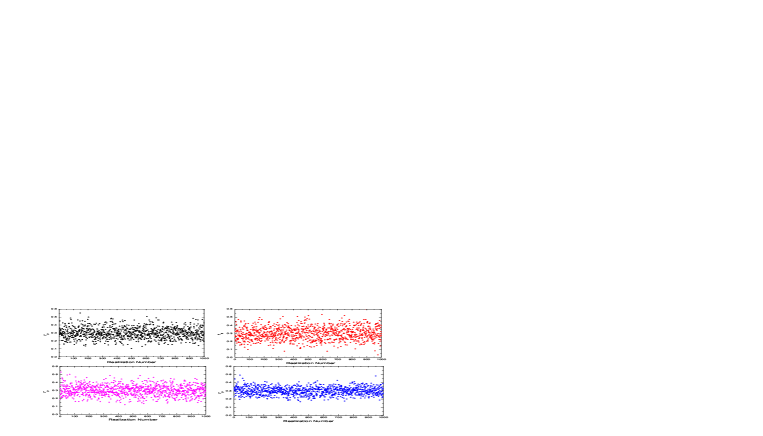
Figure 1: The distribution of $r_{p}$ in the 1000 realization. The black dots (upper left panel) denote the result in “B” case, the red dots (upper right panel) are the result in “CT” case, the magenta dots (lower left panel) are the result in “CTE” case, and the blue dots (lower right panel) denote the result in “CTEB” case. In all these panels, we have considered one free parameter $r$ in the likelihood analysis. The input simulated data are up to $\ell_{\max}=100$, and the input value is $\hat{r}=0.3$.

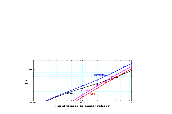
Figure 2: The value of $S/N$ depends on the input value $\hat{r}$. The black, red, magenta and blue dots (lines) are the simulation (analytic approximation) results in “B” case, “CT” case, “CTE” case and “CTEB” case, respectively.

Similar to the discussion in our previous work ours , in order to describe the detection abilities for the RGWs, we define the signal-to-noise ratio

$$S/N\equiv\hat{r}/\Delta r_{p},$$ (33)

where $\hat{r}$ is the input value of $r$. We can determine this quantity with different input $\hat{r}$. For each input, we generate $1000$ realization, and calculate the quantities $\overline{r_{p}}$, $\Delta r_{p}$ and $S/N$. The value of $S/N$ as a function of $\hat{r}$ are shown in FIG.2. From this figure, let us firstly investigate the detection abilities in the four cases. We find, in “B” case, the parameter $r$ can be determined at 2$\sigma$ level when $\hat{r}>0.06$. In “CT” case, $r$ can be determined at 2$\sigma$ level when $\hat{r}>0.16$. In “CTE” case, $r$ can be determined at 2$\sigma$ level when $\hat{r}>0.13$, and in“CTEB” case, $r$ can be determined at 2$\sigma$ level when $\hat{r}>0.05$.

From FIG.2, We can also compare the sensitivities in the different cases by the values of $S/N$. Comparing “CT” and “B”, we find the former one is more sensitive when $\hat{r}$ is large, and the latter one is more sensitive when $\hat{r}$ is small. “CT” is more sensitive than “B” when $\hat{r}>0.5$. “CTE” is more sensitive than “B”, when $\hat{r}>0.3$. In order to investigate the contribution of $E$-polarization on the detection of RGWs, we can compare the values of $S/N$ in “CT” and “CTE” cases. From the FIG.2, we find the quantity $S/N$ in “CTE” case is always $15\%$ larger than that in “CT” case. So considering the $E$-polarization, the constraint on $r$ can be improved for any $\hat{r}$. From the FIG.2, we also find that, as the combination of “CTE” and “B”, “CTEB” is more sensitive than the other three cases. When $\hat{r}$ is small, the sensitivity in “CTEB” case is close to that in “B” case, since in this case, the sensitivity of “CTE” is very weak. When $\hat{r}$ is large, the sensitivity in “CTEB” is close to that in “CTE” case.

Table 1: The mean values and standard deviations of $r_{p}$. In the likelihood analysis, we have considered one free parameter $r$.

input $\ell_{\max}$	output parameter	B	CT	CTE	CTEB
$100$	$\overline{r_{p}}\pm\Delta r_{p}$	$0.305\pm 0.067$	$0.298\pm 0.078$	$0.303\pm 0.070$	$0.304\pm 0.047$
$500$	$\overline{r_{p}}\pm\Delta r_{p}$	$0.302\pm 0.067$	$0.301\pm 0.080$	$0.302\pm 0.066$	$0.302\pm 0.047$

We have also applied the simulation method to another condition: the input quantities are all exactly same with those in Eq. (32), except the value of $\ell_{\max}$. In this case we adopt $\ell_{\max}=500$, i.e. the simulated data $D_{\ell}^{XX^{\prime}}$ in the range $\ell\leq 500$ are used for the likelihood analysis. In Table 1 we summarize the output values $\overline{r_{p}}\pm\Delta r_{p}$ in “B”, “CT”, “CTE”, “CTEB” cases, where $\hat{r}=0.3$ is used. We find that, the results in this condition is very close to those in the condition with $\ell_{\max}=100$. This result testifies that, when considering the Planck instrumental noises, the contribution of RGWs in the CMB power spectra $C_{\ell}^{XX^{\prime}}$ are important only at the large scale ($\ell\leq 100$).

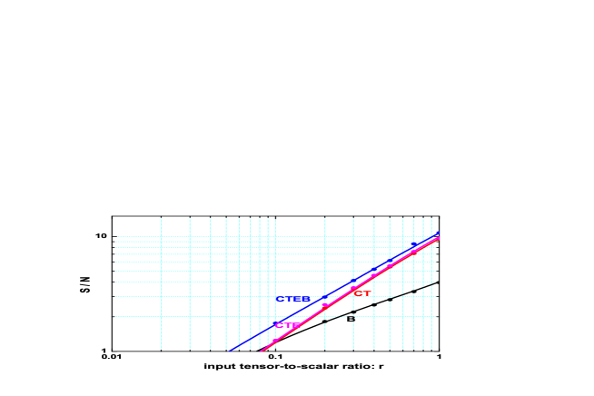
Figure 3: The same graph as in FIG.2, the only difference is that, in this figure we have assumed the realistic noise power spectra $N_{\ell}^{XX}$ are 4 times larger than the Planck instrumental noises.

To this point we have assumed that the noise power spectra only come from the Planck instrumental noise. However, synchrotron and bremsstrahlung radiation, thermal emission from cold dust, and unsolved extragalactic sources also contribute to the anisotropy and polarization of radiation. These contaminations can enlarge the effective “noises” of CMB power spectra knox ; 5map ; noises22 . In order to estimate the effect of these contaminations on the constraint of $r$, in this paper, we only simply assume the foreground will degrade the noise $a_{\ell m}^{X}(n)$ by a factor $2$. Therefore, we take into account the effect of foreground contaminations by simply increasing $N_{\ell}^{XX}$ to $4N_{\ell}^{XX}$. In this case, by the exactly same steps as the previous discussion, we recalculate the signal-to-noise ratio $S/N$ by the simulation method, where different input values $\hat{r}$ are considered. The quantity $S/N$ as a function of $\hat{r}$ in four cases are shown in FIG.3. Let us firstly discuss the results in “B” case. Comparing with the results in FIG.2, we find the detection ability in “B” case is much decreased. Only when $\hat{r}>0.25$, the signal of RGWs can be detected in 2$\sigma$ level. However, in “CT” and “CTE” cases, the results are similar with those in the previous condition with only instrumental noises (FIG.2). Comparing the sensitivities in “CT” and “CTE” cases, we find the difference is very small, which suggests that the contribution of $E$-polarization for the detection of RGWs is negligible. In “CTEB” cases, when $\hat{r}>0.12$, the signal of RGWs can be detected in 2$\sigma$ level.

In the previous work ours , we found that WMAP5 $TE$ data induces the best-fit model with $r\simeq 0.48$. From FIGs. 2 and 3, we find that RGWs with $r=0.48$ will be presented nearly at $9\sigma$ level in “CTEB” case, when the Planck instrumental noises are considered. If the assumed realistic noises are considered, it will be presented at $6\sigma$ level. These are all much better than the results in “TE” and “BB” methods ours .

V Analytic approximation of $S/N$

In Section IV, using the signal-to-noise ratio $S/N$ calculated by the simulated data, we have investigated the detection abilities for the RGWs in four cases (“B”, “CT”, “CTE”, “CTEB” cases). In order to better understand this signal-to-noise ratio and get an intuitive feel for the results in Section IV, in this section we shall give a simple analytic approximation of the signal-to-noise ratio. Similar to the discussion in Section IV, in the analytic approximation, we will also be interested in a single unfixed parameter, the tensor-to-scalar ratio $r$. Other parameters ($n_{t}$, $A_{s}$ and $n_{s}$) and background parameters ($h$, $\Omega_{b}$, $\cdot\cdot\cdot$) are all assumed to be exactly known.

V.1 Analytic approximation of the likelihood functions

In order to present the analytic expression of the signal-to-noise ratio, we need to express the likelihoods as the simple functions of variable $r$. We notice that the exact pdfs in Eqs. (13), (16), (20), (21), are all very close to the Gaussian function, especially when $\ell\gg 1$ (see for instant ours ; wishart2 ). Based on the Gaussian approximation of these pdfs, the likelihood functions in Eqs. (23), (27), (25), (29) can be simplified as (58), (65), (66), (67) (see Appendix A for the details), which can be rewritten in a unified form as follows:

$$-2\ln\mathcal{L}(r)=\sum_{\ell=2}^{\ell_{\max}}\sum_{XX^{\prime}}\left[\frac{C_{\ell}^{XX^{\prime}}-D_{\ell}^{XX^{\prime}}(\hat{r})}{\Delta D_{\ell}^{XX^{\prime}}(\hat{r})}\right]^{2}.$$ (34)

In “B” case, we have $XX^{\prime}=BB$; in “CT” case, we have $XX^{\prime}=TE,TT$; in “CTE” case, $XX^{\prime}=TE,TT,EE$; and in “CTEB” case, we have $XX^{\prime}=TE,TT,EE,BB$. In each case, the likelihood function ${\cal L}$ depends on the variable $r$ only by the power spectra $C_{\ell}^{XX^{\prime}}$.

In general, ignoring the possible contribution from the (vector) rotational perturbations, the CMB power spectra $C_{\ell}^{XX^{\prime}}$ can be presented as a sum of two contributions: density perturbations and gravitational waves:

$$C_{\ell}^{XX^{\prime}}(r)=C_{\ell}^{XX^{\prime}}(dp)+C_{\ell}^{XX^{\prime}}(gw),$$ (35)

where $C_{\ell}^{XX^{\prime}}(dp)$ and $C_{\ell}^{XX^{\prime}}(gw)$ are the contributions of density perturbations and gravitational waves, respectively. We should remember $C_{\ell}^{BB}(dp)=0$. In the likelihood analysis, we have fixed the parameters $n_{t}$, $A_{s}$, $n_{s}$ as their input values, and only considered a single free parameter $r$. $C_{\ell}^{XX^{\prime}}(gw)$ depends on the variable $r$, which can be written as

$$C_{\ell}^{XX^{\prime}}(gw)=\left(\frac{r}{\hat{r}}\right)\hat{C}_{\ell}^{XX^{\prime}}(gw),$$ (36)

where $\hat{C}_{\ell}^{XX^{\prime}}(gw)$ are the power spectra $C_{\ell}^{XX^{\prime}}(gw)$ at $r=\hat{r}$. Inserting (36) in (35), we get

$$C_{\ell}^{XX^{\prime}}(r)=C_{\ell}^{XX^{\prime}}(dp)+\left(\frac{r}{\hat{r}}\right)\hat{C}_{\ell}^{XX^{\prime}}(gw).$$ (37)

Now, let us return to the likelihood function. Inserting (37) into Eq. (34), we obtain that

$$-2\ln\mathcal{L}(r)=\sum_{\ell=2}^{\ell_{\max}}\sum_{XX^{\prime}}\alpha^{XX^{\prime}}_{\ell}\left(\frac{r}{\hat{r}}-\beta^{XX^{\prime}}_{\ell}\right)^{2},$$ (38)

where the quantities $\alpha_{\ell}^{XX^{\prime}}$ and $\beta_{\ell}^{XX^{\prime}}$ are defined by

$$\alpha^{XX^{\prime}}_{\ell}\equiv\left(\frac{\hat{C}_{\ell}^{XX^{\prime}}(gw)}{\Delta D_{\ell}^{XX^{\prime}}(\hat{r})}\right)^{2},~{}~{}\beta^{XX^{\prime}}_{\ell}\equiv\frac{D_{\ell}^{XX^{\prime}}(\hat{r})-C_{\ell}^{XX^{\prime}}(dp)}{\hat{C}_{\ell}^{XX^{\prime}}(gw)}.$$ (39)

After straight forward manipulations, the expression (38) can be rewritten as the following form

$$-2\mathcal{L}(r)=(\sum_{\ell=2}^{\ell_{\max}}\sum_{XX^{\prime}}\alpha_{\ell}^{XX^{\prime}})\left(\frac{r}{\hat{r}}-\frac{\sum_{\ell=2}^{\ell_{\max}}\sum_{XX^{\prime}}\alpha_{\ell}^{XX^{\prime}}\beta_{\ell}^{XX^{\prime}}}{\sum_{\ell=2}^{\ell_{\max}}\sum_{XX^{\prime}}\alpha_{\ell}^{XX^{\prime}}}\right)^{2}+C^{\prime},$$ (40)

where the separate part $C^{\prime}$ is independent of the variable $r$. In the following, based on this formula, we shall discuss the signal-to-noise ratio $S/N$.

V.2 Analytic approximation of $S/N$

Now, let us investigate the likelihood in (40). First, we shall discuss the peak of the likelihood function. We notice that this likelihood is a “Gaussian form function” of the variable $r$. The maximum is at $r_{p}$, which is

$$r_{p}=\frac{\sum_{\ell=2}^{\ell_{\max}}\sum_{XX^{\prime}}\alpha_{\ell}^{XX^{\prime}}\beta_{\ell}^{XX^{\prime}}}{\sum_{\ell=2}^{\ell_{\max}}\sum_{XX^{\prime}}\alpha_{\ell}^{XX^{\prime}}}\hat{r}.$$ (41)

From the definition of $\alpha_{\ell}^{XX^{\prime}}$ and $\beta_{\ell}^{XX^{\prime}}$ in Eq. (39), we find the value of $r_{p}$ not only depends on the values of $C_{\ell}^{XX^{\prime}}(\hat{r})$, the input model, and $N_{\ell}^{XX}$, the noise power spectra, but also depends on the values of $D_{\ell}^{XX^{\prime}}$, the simulated data. So for any two realization, even if generated by the exactly same input model and noises, they have the different values of $r_{p}$.

From the likelihood in Eq. (40), we can also obtain the spread of the likelihood $\Delta r$, which is

$$\Delta r=\frac{\hat{r}}{\left(\sum_{\ell=2}^{\ell_{\max}}\sum_{XX^{\prime}}\alpha_{\ell}^{XX^{\prime}}\right)^{1/2}}.$$ (42)

The spread of the likelihood only depends on the values of $C_{\ell}^{XX^{\prime}}(\hat{r})$, the input model, and $N_{\ell}^{XX}$, the noise power spectra. So we get the conclusion, for any two realization, as long as they have the same input model and noises, they have the same $\Delta r$, the spread of the likelihood function.

In the previous work ours , we have defined the signal-to-noise ratio $\widetilde{S/N}$ as

$$\widetilde{S/N}\equiv{\hat{r}}/{\Delta r}.$$ (43)

Note that, in order to distinguish from $S/N$ defined in (33), we denote the signal-to-noise ratio in our previous work as $\widetilde{S/N}$. In the following, we will find these two definitions have the exactly same values. Using the formula in (42) and the definition of $\alpha_{\ell}^{XX^{\prime}}$ in (39), we obtain

$$\widetilde{S/N}=\sqrt{\sum_{\ell=2}^{\ell_{\max}}\sum_{XX^{\prime}}\left(\frac{\hat{C}_{\ell}^{XX^{\prime}}(gw)}{\Delta D_{\ell}^{XX^{\prime}}(\hat{r})}\right)^{2}}.$$ (44)

This is the finial analytic result of the quantity $\widetilde{S/N}$, which depends on the input power spectra $C_{\ell}^{XX^{\prime}}(\hat{r})$ and the noise power spectra $N_{\ell}^{XX^{\prime}}$. In the work jaffe , by the Fisher Matrix analysis, the authors have obtained a same result as Eq. (44) in the case of $XX^{\prime}=BB$ (the result in “B” case). The results in Eqs. (41), (42) and (44) describe the constraint on the tensor-to-scalar ratio $r$, based on one set of simulated data $\{D_{\ell}^{XX^{\prime}}|\ell=2,3,\cdot\cdot\cdot,\ell_{\max}\}$.

However, in our discussion in Section IV, we have considered another case. In the simulation method, based on a same input cosmological model and noises, we have randomly generated $N$ ($N\gg 1$) realization. For each realization, we can obtain a maximum of likelihood $r_{p}$. From these $r_{p}$, we have calculated the mean value and standard deviation of $r_{p}$. From the simulation, we find the mean value $\overline{r_{p}}$ is close to the input value $\hat{r}$, and the standard deviation $\Delta r_{p}$ stands for the uncertainty of the parameter $r$, in the likelihood analysis. Now, we shall prove these in the analytic approximation.

In the analytic approximation, from Eq. (41) we can also calculate the values of $\overline{r_{p}}$ and $\Delta r_{p}$. The mean value $\overline{r_{p}}$ is

$$\overline{r_{p}}=\frac{\sum_{\ell=2}^{\ell_{\max}}\sum_{XX^{\prime}}\alpha_{\ell}^{XX^{\prime}}\langle\beta_{\ell}^{XX^{\prime}}\rangle}{\sum_{\ell=2}^{\ell_{\max}}\sum_{XX^{\prime}}\alpha_{\ell}^{XX^{\prime}}}\hat{r}.$$ (45)

Considering the definition of $\beta_{\ell}^{XX^{\prime}}$ in Eq. (39), the relation $\langle D_{\ell}^{XX^{\prime}}(\hat{r})\rangle=C_{\ell}^{XX^{\prime}}(\hat{r})$ and the Eq. (37), we can obtain that $\langle\beta_{\ell}^{XX^{\prime}}\rangle=1$. Inserting it into Eq. (45), we get a relation

$$\overline{r_{p}}=\hat{r}.$$ (46)

This relation suggests that, the mean value of $r_{p}$ is equal to the input value $\hat{r}$, which is consistent with the simulation result in Section IV.

We can also discuss the standard deviation of $r_{p}$, which is defined by $\Delta r_{p}\equiv\sqrt{\overline{r_{p}^{2}}-{\overline{r_{p}}}^{2}}$. Using Eq. (41) and the relation $\langle D_{\ell}^{XX^{\prime}}(\hat{r})\rangle=C_{\ell}^{XX^{\prime}}(\hat{r})$, after a straight forward manipulations, we obtain that

$$\Delta r_{p}=\frac{\hat{r}}{\left(\sum_{\ell=2}^{\ell_{\max}}\sum_{XX^{\prime}}\alpha_{\ell}^{XX^{\prime}}\right)^{1/2}}.$$ (47)

Comparing (47) with (42), we find $\Delta r_{p}=\Delta r$. By the formula (47), we can discuss the signal-to-noise ratio $S/N$, defined by Eq. (33). Taking into account the definition of $\alpha_{\ell}^{XX^{\prime}}$ in Eq. (39), we can write the signal-to-noise ratio as

$$S/N=\widetilde{S/N}=\sqrt{\sum_{\ell=2}^{\ell_{\max}}\sum_{XX^{\prime}}\left(\frac{\hat{C}_{\ell}^{XX^{\prime}}(gw)}{\Delta D_{\ell}^{XX^{\prime}}(\hat{r})}\right)^{2}},$$ (48)

which depends on the input power spectra $C_{\ell}^{XX^{\prime}}(\hat{r})$ and the noise power spectra $N_{\ell}^{XX^{\prime}}$. In Eq. (48), we should remember that, $XX^{\prime}=BB$ in “B” case, $XX^{\prime}=TE,TT$ in “CT” case, $XX^{\prime}=TE,TT,EE$ in “CTE” case and $XX^{\prime}=TE,TT,EE,BB$ in “CTEB” case. From the expression in (48), we find that, the two definitions of signal-to-noise ratio, $S/N$ and $\widetilde{S/N}$ have the same values. They all stand for the detection abilities for the RGWs.

Using Eq. (48), and taking into account the corresponding noises power spectra $N_{\ell}^{XX^{\prime}}$, in FIG.2 and 3, we have plotted the quantities $S/N$ as a function of $\hat{r}$ in “B”, “CT”, “CTE”, “CTEB” cases. We find they are all exactly consistent with the simulation results.

V.3 Understanding the analytic approximation of $S/N$

Now, let us investigate the approximation formula (48), which can be rewritten as

$$(S/N)^{2}=(\widetilde{S/N})^{2}={\sum_{\ell=2}^{\ell_{\max}}\sum_{XX^{\prime}}\left(\frac{\hat{C}_{\ell}^{XX^{\prime}}(gw)}{\Delta D_{\ell}^{XX^{\prime}}(\hat{r})}\right)^{2}}.$$ (49)

In this expression, $\hat{C}_{\ell}^{XX^{\prime}}(gw)$ is the contribution of RGWs to the total power spectra, which determines the strength of the signal of RGWs. $\Delta D_{\ell}^{XX^{\prime}}$ is the uncertainty of the estimator, which serves as the corresponding ‘noises’. So the total signal-to-noise ratio $S/N$ (or $\widetilde{S/N}$) is determined by the sum of the ratios between RGWs signal and the corresponding ‘noise’ at every multipole and $XX^{\prime}$. This result is consistent with that in “TE” method, which has been obtained in our previous work ours .

From Eq. (49), we can discuss the contribution of each $\ell$ to the total signal-to-noise ratio. We define the signal-to-noise ratio at the individual multipole $\ell$, $(S/N)_{\ell}$ as below:

$$(S/N)_{\ell}^{2}\equiv\sum_{XX^{\prime}}\left(\frac{\hat{C}_{\ell}^{XX^{\prime}}(gw)}{\Delta D_{\ell}^{XX^{\prime}}(\hat{r})}\right)^{2}.$$ (50)

Thus the total signal-to-noise ratio can be written as the following sum:

$$(S/N)^{2}=(\widetilde{S/N})^{2}=\sum_{\ell=2}^{\ell_{\max}}(S/N)^{2}_{\ell}.$$ (51)

Let us discuss the quantity $(S/N)_{\ell}^{2}$. Taking into account the noise power spectra $N_{\ell}^{XX^{\prime}}$, and adopt the input value $\hat{r}=0.3$, in FIG. 4 we plot the quantity $(S/N)_{\ell}^{2}$ as a function of $\ell$. Let us firstly focus on the lines in “B” case (black lines). We find that $(S/N)_{\ell}^{2}$ is sharply peaked at $\ell<10$. As mentioned in our previous work ours , the main contribution in “B” case comes from the signal in the range $\ell<10$. Especially, by comparing the line in left panel (Planck instrumental noises are considered) with the right panel (noise power spectra are 4 times larger than Planck instrumental noises), we find when increasing the noise power spectra, the value of $(S/N)_{\ell}^{2}$ reduces by a factor $2$, at the scale $\ell<10$. However, at the scale $\ell>10$, the value of $(S/N)_{\ell}^{2}$ reduces by a factor $10$. So we get the conclusion, when increasing the noise power spectra, in “B” case, the contribution from $\ell<10$ becomes more and more dominant. Since in the range $\ell<10$, the $BB$ power spectra $C_{\ell}^{BB}$ are mainly generated by the cosmic reioniztion a11 ; a12 , the sensitivity in “B” case strongly depends on the cosmic reionization process.

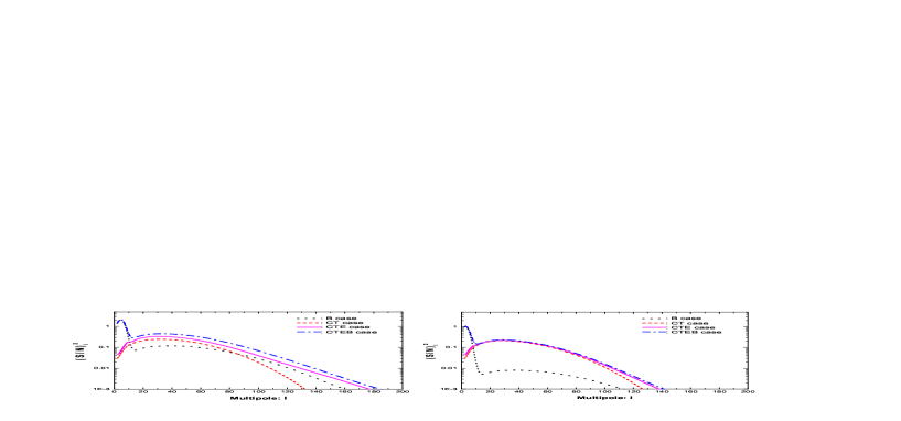
Figure 4: This figure shows the individual signal-to-noise ratio $(S/N)_{\ell}^{2}$ as a function of $\ell$. The presented in left panel is the result with the Planck instrumental noises, and the presented in right panel is the result in the case where we assume the realistic noise power spectra $N_{\ell}^{XX}$ are 4 times larger than the Planck instrumental noises.

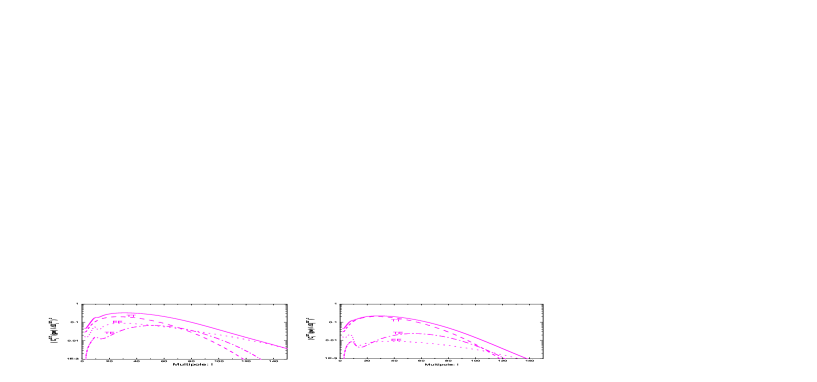
Figure 5: This figure shows three quantities of $(\hat{C}_{\ell}^{XX^{\prime}}(gw)/\Delta D_{\ell}^{XX^{\prime}})^{2}$ ($XX^{\prime}=TE,TT,EE$) as a function of $\ell$. As the combination of these three components, the individual signal-to-noise ratio $(S/N)_{\ell}^{2}$ in “CTE” case are plotted in solid lines. In the left panel, we have considered the Planck instrumental noises, and in the right panel, we have assumed the realistic noise power spectra are 4 time larger than the Planck instrumental noises.

Let us turn to the the quantity $(S/N)_{\ell}^{2}$ in “CT” and “CTE” cases, which are plotted in red (dashed) and magenta (solid) lines in FIG.4. We find that, in both panels of FIG.4, the quantities $(S/N)_{\ell}^{2}$ in “CT” and “CTE” cases, are all peaked at $\ell\sim 30$. Among the total $S/N$, the main contribution comes from the intermedial range $10<\ell<70$. In the very large scale $\ell<10$ and the small scale $\ell>70$, the values of $(S/N)_{\ell}^{2}$ are all very small. Their contributions to the total $S/N$ are negligible. Since $(S/N)_{\ell}^{2}$ is very small in the scale $\ell<10$, the influence of cosmic reionization on the detection abilities are also not obvious, which is same with the “TE” method, but different from the “BB” method. By comparing the solid and dashed lines in the left panel with the corresponding lines in the right panel, we find that, increasing the noises, the values of $(S/N)_{\ell}^{2}$ in “CT” and “CTE” cases have no obvious change, which induces that the total $S/N$ in “CT” and “CTE” cases have no obvious change (see FIG.2 and 3).

From Eq. (50), we find, in “CTE” (or “CT”) case, the quantity $(S/N)_{\ell}^{2}$ is a simple sum of the portions with $XX^{\prime}=TE$, $TT$ and $EE$. So we can also discuss their contributions to the quantity $(S/N)_{\ell}^{2}$ separately. In FIG.5, we plot these three portions of $(S/N)_{\ell}^{2}$ in dash-dotted lines, dashed lines, and dotted lines. In this figure, the solid lines denote the sum of these three portions, which exactly corresponds to the magenta lines in FIG.4. We find, when considering the Planck instrumental noises, these three portions are close to each. In the range $10<\ell<70$, the largest contribution comes from the component $XX^{\prime}=TT$, which is 2 or 3 times larger than the components $XX^{\prime}=TE$ and $XX^{\prime}=EE$. However, in the case with large noises (right panel in FIG.5), the contributions of the component $XX^{\prime}=EE$ rapidly decreases, and becomes negligible among the quantity $(S/N)_{\ell}^{2}$, which induces that the value of the quantity $(S/N)_{\ell}^{2}$ in “CTE” case are very close to that in “CT” case (see the right panel of FIG.4). So the total $S/N$ in “CTE” and “CT” cases are also very close to each other (see FIG.3).

We can also discuss the quantity $(S/N)_{\ell}^{2}$ in “CTEB” case, which are plotted in blue (dash-dotted) lines in FIG.4. From Eq. (50), we find the quantity $(S/N)_{\ell}^{2}$ in “CTEB” case is a simple sum of $(S/N)_{\ell}^{2}$ in “CTE” case and in “B” case. In the range of $\ell<10$, the quantity $(S/N)_{\ell}^{2}$ in “CTEB” case is close to that in “B” case, and in the range of $\ell>10$, it is close to that in “CTE” case.

VI Effects of free parameters: $n_{t}$ and $A_{s}$, $n_{s}$

In the previous sections, by both the simulation and the analytic approximation, we have discussed the constraints of the tensor-to-scalar ratio $r$ in “B”, “CT”, “CTE”, “CTEB” cases. However, in the real detection, we always have to constrain all the cosmic parameters, including $h$ the Hubble parameter, $\Omega_{b}$ the baryon density, $\Omega_{m}$ the matter density, $\Omega_{k}$ the spatial curvature, $\tau_{reion}$ the reionization optical depth. The parameters also include the scalar spectrum parameters: $A_{s}$ the amplitude of scalar spectrum and $n_{s}$ the scalar spectral index, and the tensor spectrum parameters: $r$ the tensor-to-scalar ratio and $n_{t}$ the tensor spectral index.

As mentioned in Section IV, in all this paper, we shall not consider the constraints of the background cosmological parameters, and assume they have been exactly determined. In the likelihood analysis in Sections IV and V, we have considered the case with only one free parameter $r$. The other parameters $n_{t}$, $A_{s}$ and $n_{s}$ are all fixed as their input values. Based on this assumption, we have discussed the constraint on $r$ in “B”, “CT”, “CTE”, “CTEB” cases. Thus a question arises, if the parameters, $n_{t}$, $A_{s}$, $n_{s}$ are also set free in the likelihood analysis, whether they can influence the constraint on the parameter $r$.

In this section, by the simulation method, we shall answer this question. In the Section VI.1, we shall discuss the constraints on the free parameters, $r$ and $n_{t}$, and investigate the effect of $n_{t}$ on the constraint of $r$. In Section VI.2, we shall consider the free parameters $r$, $n_{t}$, $A_{s}$ and $n_{s}$, and investigate the effects of $A_{s}$ and $n_{s}$ on the constraint of $r$.

VI.1 Effect of the free parameter $n_{t}$

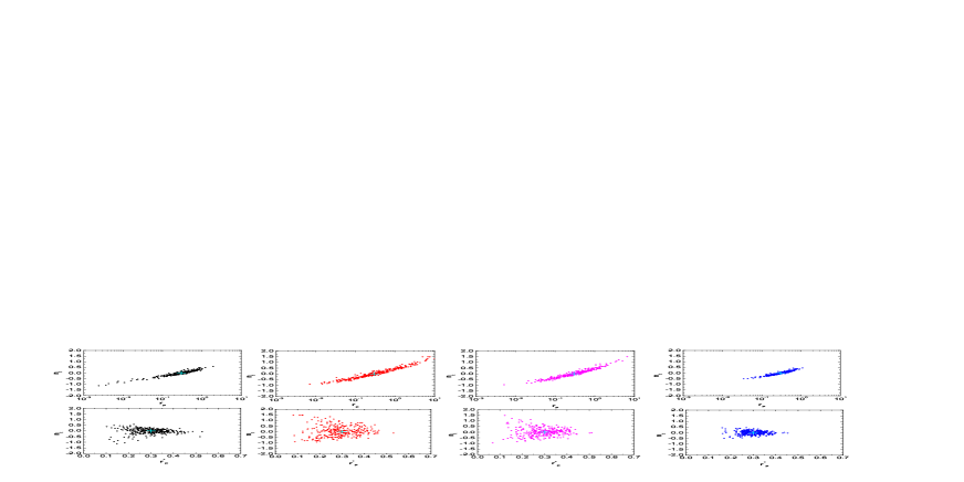
Figure 6: The locations of the maxima from 300 realization projected into $n_{t}-r_{p}$ (upper panels), and $n_{t}-r_{p}^{*}$ (lower panels) planes. Black (red, magenta, blue) dots denote the results in “B” (“CT”, “CTE”, “CTEB”) case. In all these graphs, we have considered two free parameters ($r$, $n_{t}$) in the likelihood analysis. The input simulated data are up to $\ell_{\max}=100$, and the sign $``+"$ denotes the input values of the parameters.

Here, we shall use the simulation method described in Section IV.1. We choose the parameters $r$ and $n_{t}$ as the unfixed parameters, $A_{s}$ and $n_{s}$ as the fixed parameters. The values of $\ell_{\max}$, $N$ and the input values of parameters are adopted as the follows:

$$\ell_{\max}=100,~{}~{}N=300,~{}~{}\hat{r}=0.3,~{}~{}\hat{n}_{t}=0.0,~{}~{}\hat{A}_{s}=2.3\times 10^{-9},~{}~{}\hat{n}_{s}=1.0.$$ (52)

The background cosmological parameters are adopt as in Eq. (31). We consider the Planck instrumental noises and Planck window function, which are given in Eqs. (7a-7d). $N=300$ suggests that our following simulation results ($\overline{r_{p}}$, $\Delta r_{p}$, $\overline{n_{t}}$, $\Delta n_{t}$) have $4\%$ statistical error.

As mentioned above ($n_{s}=1$ and $n_{t}=0$), for any two different pivot wavenumbers $k_{0}$ and $k_{1}$, the tensor-to-scalar ratio $r(k_{0})$ and $r(k_{1})$ have the different constraints, due to the free parameter $n_{t}$. Although they have the same input values $\hat{r}=0.3$, due to the formula in (4) and $\hat{n}_{t}-\hat{n}_{s}+1=0$. As the first step, in the likelihood analysis, we choose the pivot wavenumber

$$k_{0}=0.05{\rm Mpc}^{-1}.$$ (53)

Presented in FIG.6 (upper panels) shows the maxima projected into $n_{t}-r_{p}$ plane from $300$ realization. First, we discuss the “B” case. The result is $\overline{r_{p}}\pm\Delta r_{p}=0.351\pm 0.235$. The uncertainty of $r$ becomes nearly four times larger than the previous one (the result in the case with fixed $n_{t}$), due to the free tensor spectral index $n_{t}$. The constraint on $n_{t}$ is: $\overline{n_{t}}\pm\Delta n_{t}=-0.022\pm 0.240$.

From FIG.6, we also find the strong correlation between $n_{t}$ and $r_{p}$, which can be easily understood. It is due to we have chosen the pivot scale $k_{0}=0.05$Mpc^-1. However, the quantity $r$ in this scale, $r(k_{0})$, is not the one which is measured most precisely. We assume that there is a tensor-to-scalar ratio $r^{*}(k_{t}^{*})$ (the tensor-to-scalar ratio at the pivot wavenumber $k_{t}^{*}$), which can be measured most precisely. We expect this quantity $r^{*}(k_{t}^{*})$ has no correlation with $n_{t}$. In this paper, we call $k_{t}^{*}$ as the ‘best pivot wavenumber’. Following Eq. (4), we can relate $r^{*}(k_{t}^{*})$ and $r(k_{0})$ by the following formula

$$r(k_{0})=r^{*}(k_{t}^{*})\left(\frac{k_{0}}{k_{t}^{*}}\right)^{n_{t}}.$$ (54)

Since in the calculation, we have adopted the input tensor spectral index $\hat{n}_{t}=0$, we have $\hat{r}^{*}(k_{t}^{*})=\hat{r}(k_{0})=0.3$. However, the uncertainties of these two quantities ($r^{*}$ and $r$) are expected to be different.

Table 2: The best pivot wavenumber $k_{t}^{*}$, the mean values and the standard deviations of ($r_{p}$, $n_{t}$, $r_{p}^{*}$). In the likelihood analysis, we have considered two free parameters ($r$, $n_{t}$).

input $\ell_{\max}$	output parameter	B	CT	CTE	CTEB
$100$	$k^{*}_{t}$(Mpc-1)	$1.26\times 10^{-3}$	$3.13\times 10^{-3}$	$3.43\times 10^{-3}$	$2.25\times 10^{-3}$
$100$	$\overline{r^{*}_{p}}\pm\Delta r^{*}_{p}$	$0.296\pm 0.072$	$0.288\pm 0.081$	$0.293\pm 0.073$	$0.300\pm 0.049$
$100$	$\overline{n_{t}}\pm\Delta n_{t}$	$-0.022\pm 0.240$	$0.051\pm 0.475$	$0.023\pm 0.369$	$-0.003\pm 0.166$
$100$	$\overline{r_{p}}\pm\Delta r_{p}$	$0.351\pm 0.235$	$0.775\pm 1.329$	$0.502\pm 0.678$	$0.335\pm 0.167$
$500$	$k^{*}_{t}$(Mpc-1)	$1.52\times 10^{-3}$	$2.97\times 10^{-3}$	$3.75\times 10^{-3}$	$2.37\times 10^{-3}$
$500$	$\overline{r^{*}_{p}}\pm\Delta r^{*}_{p}$	$0.291\pm 0.066$	$0.291\pm 0.083$	$0.293\pm 0.067$	$0.298\pm 0.046$
$500$	$\overline{n_{t}}\pm\Delta n_{t}$	$-0.016\pm 0.226$	$-0.024\pm 0.433$	$-0.019\pm 0.327$	$-0.009\pm 0.159$
$500$	$\overline{r_{p}}\pm\Delta r_{p}$	$0.352\pm 0.249$	$0.559\pm 0.950$	$0.399\pm 0.414$	$0.325\pm 0.172$

We use the following steps to search for the best pivot wavenumber $k_{t}^{*}$:

Step 1 Randomly choose a pivot wavenumber $k^{\prime}$, which is different from $k_{0}$.

Step 2 Calculate the value of $r_{p}(k^{\prime})$ by the formula in Eq. (4).

Step 3 Project the maxima of the likelihood functions for $300$ realization into $n_{t}-r_{p}(k^{\prime})$ plane.

Step 4 In $n_{t}-r_{p}(k^{\prime})$ plane, if $r_{p}(k^{\prime})$ correlates with $n_{t}$, we iterate the same steps from Step 1. Otherwise, if $r_{p}(k^{\prime})$ has the weakest correlation with $n_{t}$, we get the result: $k^{\prime}=k_{t}^{*}$, and $r_{p}(k^{\prime})=r_{p}^{*}(k_{t}^{*})$.

By these four steps, we find, in “B” case, the best pivot wavenumber is $k_{t}^{*}=1.26\times 10^{-3}$Mpc^-1. In FIG.6, we plot the distribution of $n_{t}-r_{p}^{*}$ (left lower panel). As expected, the correlation between $n_{t}$ and $r_{p}^{*}$ disappears. We also calculate the average value and standard deviation of $r_{p}^{*}$, which is $\overline{r_{p}^{*}}\pm\Delta r_{p}^{*}=0.296\pm 0.072$. The average value of $r_{p}^{*}$ is equal to the input value $\hat{r^{*}}=0.3$ within $1\%$ and hence there is no evidence for bias. The standard deviation of $r_{p}^{*}$ ($\Delta r_{p}^{*}=0.072$) is much smaller than that of $r_{p}$ ($\Delta r_{p}=0.235$), but close to the result $\Delta r_{p}=0.067$ gotten in Section IV, where only free parameter $r$ is considered. Hence we conclude that, if we choose the best pivot wavenumber, the free parameter $n_{t}$ cannot influence the constraint on the tensor-to-scalar ratio.

We can also consider the constraints on $r$ and $n_{t}$ in the other cases. The distributions of $r_{p}$ and $n_{t}$ in the $300$ realization are all plotted in FIG.6 (upper panels). The strong correlations exist in all these panels. By the exactly same steps, we can find the best wavenumber $k_{t}^{*}$, which are all listed in Table 2. For example, in “CT” case $k_{t}^{*}=3.13\times 10^{-3}$Mpc^-1 and in “CTE” case $k_{t}^{*}=3.43\times 10^{-3}$Mpc^-1. In these two cases, the best pivot wavenumbers are close to each other, which are all much larger than that in “B” case. In “CTEB” case, the best pivot wavenumber is $k_{t}^{*}=2.25\times 10^{-3}$Mpc^-1, which is between that in “B” case and that in “CTE” case. In all these three cases, the values of $\Delta r_{p}^{*}$ are all very close to that of $\Delta r_{p}$ gotten in Section IV, when only free parameter $r$ is considered. Hence, we obtain the same conclusion, if we adopt the best pivot wavenumber, the free parameter $n_{t}$ cannot expand the constraint on the tensor-to-scalar ratio (We should mention that, in the latter work our3 , we have completely proved this conclusion, and given the analytic formulae for the best pivot wavenumber $k_{t}^{*}$ and the uncertainty $\Delta n_{t}$).

From Table 2, we also find that, the uncertainty of $n_{t}$ is always very large. For example in “CTEB” case, the constraint is $\Delta n_{t}=0.166$, which is fairly loose for the determination of the physical model of the early universe.

We have also considered another condition, where a broader range ($\ell_{\max}=500$) simulated data $D_{\ell}^{XX^{\prime}}$ are used for the likelihood analysis. The results are all listed in Table 2. As expected, we find that in this condition, the values of $k_{t}^{*}$ $\Delta r_{p}^{*}$, $\Delta n_{t}$ are all close to those in the previous condition, where only simulated data in large scale ($\ell_{\max}=100$) are considered.

VI.2 Effect of the free parameters $A_{s}$, $n_{s}$

In this subsection, we shall extend the discussion in Section VI.1 to the more general case, where we consider four free parameters: ($r$, $n_{t}$, $A_{s}$, $n_{s}$). By the simulated data, we can investigate the effects of free parameters $A_{s}$ and $n_{s}$ on the constraint of $r$. The steps are exactly same with that in the Section VI.1. For the simplification, we shall use the parameter $A^{\prime}_{s}$, defined by $A^{\prime}_{s}\equiv A_{s}/2.3\times 10^{-9}$, instead of $A_{s}$.

We notice that, the power spectra $C_{\ell}^{BB}$ only depends on $P_{t}(k)$, but not on $P_{s}(k)$. Since $P_{t}(k)$ is determined by the parameters $A_{t}=(rA_{s})$ and $n_{t}$, in “B” case we cannot constrain the separate parameters: $r$, $n_{t}$, $A^{\prime}_{s}$ and $n_{s}$. So in this subsection, we shall not discuss the “B” case.

We firstly consider the condition, where the values of $\ell_{\max}$, $N$, and the input values of parameters are adopted as in (52). We adopt the pivot wavenumber as in (53). The likelihood functions peak at $(r_{p},n_{t},A^{\prime}_{s},n_{s})$. FIG.7 presents the maxima projected into $n_{t}-r_{p}$ plane from $300$ realization. We find the strong correlation between $n_{t}$ and $r_{p}$ exists, which is because we have used the pivot wavenumber $k_{0}=0.05$Mpc^-1. The outputs $\overline{r_{p}}\pm\Delta r_{p}$, $\overline{n_{t}}\pm\Delta n_{t}$, $\overline{A^{\prime}_{s}}\pm\Delta A^{\prime}_{s}$, $\overline{n_{s}}\pm\Delta n_{s}$ in “CT”, “CTE”, “CTEB” cases are all listed in Table 3. We find, due to the uncertainties of $A^{\prime}_{s}$ and $n_{s}$, the values of $\Delta r_{p}$ and $\Delta n_{t}$ are all larger than the corresponding results in Table 2.

Similar to Section VI.1, we can discuss $r^{*}(k_{t}^{*})$, the tensor-to-scalar ratio at the best pivot wavenumber $k_{t}^{*}$. Following Eq. (4), we can relate $r^{*}(k_{t}^{*})$ and $r(k_{0})$ by the following formula

$$r(k_{0})=r^{*}(k_{t}^{*})\left(\frac{k_{0}}{k_{t}^{*}}\right)^{n_{t}-n_{s}+1}.$$ (55)

Since in the calculation, we have adopted the input spectral index $\hat{n}_{t}=0$ and $\hat{n}_{s}=1$, we find $\hat{r}^{*}=\hat{r}=0.3$. However, the uncertainties of $r^{*}$ and $r$ are expected to be different.

We search for the best pivot wavenumber $k_{t}^{*}$ by the exactly same steps, listed in Section VI.1. In “CT” case, the best pivot wavenumber is $k_{t}^{*}=3.11\times 10^{-3}$Mpc^-1. Based on this pivot wavenumber, we find $\Delta r^{*}_{p}=0.127$. Comparing with the result of $\Delta r^{*}_{p}=0.081$, where only two free parameters $r$ and $n_{t}$ are considered, the value of $\Delta r^{*}_{p}$ increases by $60\%$, due to the free parameters $A^{\prime}_{s}$ and $n_{s}$. Since we have only used the simulated in the large scale $\ell\leq 100$ in the likelihood analysis, the uncertainties of $A^{\prime}_{s}$ and $n_{s}$ are fairly large (see Table 3). This makes the value $\Delta r^{*}_{p}$ is obviously increased.

We have also considered the condition, where $\ell_{\max}=500$ is adopted. We find the constraints on $A^{\prime}_{s}$ and $n_{s}$ become much smaller: $\Delta A^{\prime}_{s}=0.005$ and $\Delta n_{s}=0.008$, and the constraint on $r_{p}^{*}$ becomes $\Delta r^{*}_{p}=0.091$, i.e. the influence of $A^{\prime}_{s}$ and $n_{s}$ on the constraint of $r_{p}^{*}$ becomes much smaller (increasing the value of $\Delta r_{p}^{*}$ only by $10\%$).

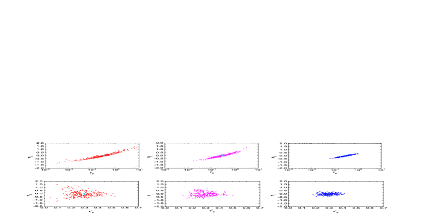
Figure 7: The locations of the maxima from 300 realization projected into $n_{t}-r_{p}$ (upper panels), and $n_{t}-r^{*}_{p}$ (lower panels) planes. Red (magenta, blue) dots denote the results in “CT” (“CTE”, “CTEB”) case. In all these graphs, we have considered four free parameters ($r$, $n_{t}$, $A^{\prime}_{s}$, $n_{s}$) in the likelihood analysis. The input simulated data are up to $\ell_{\max}=500$, and the sign $``+"$ denotes the input values of the parameters.

Table 3: The best pivot wavenumber $k_{t}^{*}$, the mean values and the standard deviations of ($r_{p}$, $n_{t}$, $r_{p}^{*}$, $A^{\prime}_{s}$, $n_{s}$). In the likelihood analysis, we have considered four free parameters ($r$, $n_{t}$, $A^{\prime}_{s}$, $n_{s}$).

input $\ell_{\max}$	output parameter	CT	CTE	CTEB
$100$	$k^{*}_{t}$(Mpc-1)	$3.11\times 10^{-3}$	$3.66\times 10^{-3}$	$2.33\times 10^{-3}$
$100$	$\overline{r^{*}_{p}}\pm\Delta r^{*}_{p}$	$0.291\pm 0.127$	$0.295\pm 0.115$	$0.300\pm 0.069$
$100$	$\overline{n_{t}}\pm\Delta n_{t}$	$-0.003\pm 0.509$	$0.009\pm 0.425$	$-0.010\pm 0.176$
$100$	$\overline{r_{p}}\pm\Delta r_{p}$	$0.783\pm 1.693$	$0.546\pm 0.838$	$0.331\pm 0.178$
$100$	$\overline{n_{s}}\pm\Delta n_{s}$	$1.006\pm 0.052$	$1.004\pm 0.050$	$1.001\pm 0.043$
$100$	$\overline{A^{\prime}_{s}}\pm\Delta A^{\prime}_{s}$	$1.016\pm 0.092$	$1.012\pm 0.090$	$1.006\pm 0.078$
$500$	$k^{*}_{t}$(Mpc-1)	$3.02\times 10^{-3}$	$3.35\times 10^{-3}$	$2.22\times 10^{-3}$
$500$	$\overline{r^{*}_{p}}\pm\Delta r^{*}_{p}$	$0.290\pm 0.091$	$0.294\pm 0.078$	$0.297\pm 0.051$
$500$	$\overline{n_{t}}\pm\Delta n_{t}$	$-0.024\pm 0.442$	$-0.053\pm 0.291$	$-0.016\pm 0.155$
$500$	$\overline{r_{p}}\pm\Delta r_{p}$	$0.570\pm 0.990$	$0.341\pm 0.341$	$0.316\pm 0.166$
$500$	$\overline{n_{s}}\pm\Delta n_{s}$	$1.000\pm 0.008$	$0.999\pm 0.008$	$0.999\pm 0.007$
$500$	$\overline{A^{\prime}_{s}}\pm\Delta A^{\prime}_{s}$	$0.999\pm 0.005$	$0.999\pm 0.005$	$0.999\pm 0.005$

In “CTE” and “CTEB” cases, we have also investigated the effects of free parameters $A^{\prime}_{s}$ and $n_{s}$ on the constraint of $r_{p}^{*}$. The results are all similar with those in “CT” case. The $n_{t}-r_{p}$ and $n_{t}-r_{p}^{*}$ planes are all plotted in FIG.7. We find in both cases, $r_{p}$ strongly correlates with $n_{t}$. However, as expected, $r_{p}^{*}$ does not correlate with $n_{t}$. The best pivot wavenumber $k_{t}^{*}$ and the constraints of the parameters are all listed in Table 3. Based on these, we conclude that: In the likelihood analysis, if we only consider the simulated data in the large scale ($\ell\leq 100$), the constraints of $r^{*}_{p}$ and $n_{t}$ become much looser, due to the uncertainty of $n_{s}$ and $A^{\prime}_{s}$. However, if we considered the simulated data in the larger range ($\ell\leq 500$), the constraints on $r^{*}_{p}$ and $n_{t}$ only increase by $\sim 10\%$. Expectable, in the likelihood analysis, if the simulated data in the range $\ell<2000$ (the real $TT$, $TE$ and $EE$ data, especially the $TT$ data, in this range are expected to be well observed by Planck satellite Planck ) are used, the influence of $A^{\prime}_{s}$ and $n_{s}$ on the values of $\Delta r_{p}^{*}$ and $\Delta n_{t}$ will become negligible.

VII Conclusion

The upcoming observations of Planck satellite provide a very possible opportunity to detect RGWs in the CMB power spectra. In this paper, by both the simulation and the analytic approximation methods, we have discussed the detection abilities for RGWs in four (“B”, “CT”, “CTE”, “CTEB”) cases. The main conclusion can be summarized as: 1) In “B” (“CT”, “CTE”, “CTEB”) case, the Planck satellite can detect the signal of RGWs at 2$\sigma$ level when $r>0.06$ ($r>0.16$, $r>0.13$, $r>0.05$). 2) Comparing “CTE” with “B”, we find that, when $r>0.3$, the value of the signal-to-noise ratio $S/N$ is larger in “CTE” case, and when $r<0.3$, the value of $S/N$ is larger in “B” case. If the realistic noise power spectra of Planck satellite is enlarged for some reasons, the value of $S/N$ in “B” case will be much reduced. However, in “CTE” case, the value of $S/N$ is little influenced. 3) The value of $S/N$ is much larger in “CTEB” case than that in “B” case, especially when $r>0.1$. 4) The free parameters $n_{t}$, $n_{s}$ and $A_{s}$, cannot reduce the value of $S/N$, if we consider the data in a large range and adopt the best pivot scale.

Acknowledgement:

The author thanks D.Baskaran for helpful discussion, and L.P.Grishchuk for the comment and helpful suggestion on the draft. This work is partly supported by Chinese NSF under grant Nos. 10703005 and 10775119. In this paper, we have used the CAMB code camb to calculate the CMB power spectra.

Appendix A Gaussian approximations of the likelihood functions

In this appendix, by using the Gaussian approximation of the pdfs for the estimators $D_{\ell}^{XX^{\prime}}$, we shall simplify the exact likelihood functions, given in Section III.

A.1 Approximation of $\mathcal{L}_{\rm B}$

First, let us focus on the analytic approximation of $\mathcal{L}_{\rm B}$. We use the following Gaussian function $f_{G}(D_{\ell}^{BB})$ to approximate the exact pdf $f(D_{\ell}^{BB})$,

$$f_{G}(D_{\ell}^{BB}(\hat{r}))=\frac{1}{\sqrt{2\pi}\Delta D_{\ell}^{BB}(\hat{r})}\exp\left[-\frac{(D_{\ell}^{BB}(\hat{r})-C_{\ell}^{BB})^{2}}{2(\Delta D_{\ell}^{BB}(\hat{r}))^{2}}\right].$$ (56)

Inserting this formula into Eq. (23), we obtain that wishart2

$$\mathcal{L}_{\rm B}(r)=C\prod_{\ell=2}^{\ell_{\max}}\left\{\frac{1}{\sqrt{2\pi}\Delta D_{\ell}^{BB}(\hat{r})}\exp\left[-\frac{(D_{\ell}^{BB}(\hat{r})-C_{\ell}^{BB})^{2}}{2(\Delta D_{\ell}^{BB}(\hat{r}))^{2}}\right]\right\},$$ (57)

where $C$ is the constant for the normalization of the likelihood function, $D_{\ell}^{BB}(\hat{r})$ is the data, based on the input tensor-to-scalar ratio $\hat{r}$. $\Delta D_{\ell}^{BB}(\hat{r})$ is the standard deviation of $D_{\ell}^{BB}(\hat{r})$. We should mention that, as a kind of approximation, Eq. (57) can give results consistent with the exact likelihood function (the detailed discussion can be found in wishart2 ).

Up to a constant, we can rewritten the likelihood (57) as follows:

$$-2\ln\mathcal{L}_{\rm B}(r)=\sum_{\ell=2}^{\ell_{\max}}\left[\frac{C_{\ell}^{BB}-D_{\ell}^{BB}(\hat{r})}{\Delta D_{\ell}^{BB}(\hat{r})}\right]^{2},$$ (58)

which includes the variable $r$ only by the power spectrum $C_{\ell}^{BB}$.

A.2 Approximation of $\mathcal{L}_{\rm CTE}$

Before proceeding on the “CT” case, let us firstly focus on the analytic approximation in “CTE” case. The likelihood function $\mathcal{L}_{\rm CTE}$ depends on the pdf $f(D_{\ell}^{TE},f_{\ell}^{TT},C_{\ell}^{EE})$, which is the Wishart function in Eq. (16). Similar to the approximation of $f(D_{\ell}^{BB})$, here we shall use the following multivariate normal function to approximate the exact Wishart distribution function:

$$f_{G}(\vec{D_{\ell}})=\frac{1}{(2\pi)^{3/2}|\Sigma|^{1/2}}\exp\left[-\frac{1}{2}(\vec{D_{\ell}}-\vec{C_{\ell}})^{\rm T}\Sigma^{-1}(\vec{D_{\ell}}-\vec{C_{\ell}})\right],$$ (59)

where the vectors $\vec{D_{\ell}}$ and $\vec{C_{\ell}}$ are defined as $\vec{D_{\ell}}\equiv[D_{\ell}^{TE}(\hat{r}),D_{\ell}^{TT}(\hat{r}),D_{\ell}^{EE}(\hat{r})]^{\rm T}$, $\vec{C_{\ell}}\equiv[C_{\ell}^{TE},C_{\ell}^{TT},C_{\ell}^{EE}]^{\rm T}$. $\Sigma$ is the covariance matrix of the variable $\vec{D_{\ell}}$. Based on the Gaussian assumption of the CMB field, the estimators $D_{\ell}^{XX^{\prime}}$ have covariance as below (see for instant covariance ; wishart2 )

$${\rm cov}(D_{\ell}^{TT},D_{\ell}^{TT}) = \frac{2(C_{\ell}^{TT}+N_{\ell}^{TT}W_{\ell}^{-2})^{2}}{(2\ell+1)f_{\rm sky}},~{}~{}$$ (60a)

$$\ {\rm cov}(D_{\ell}^{EE},D_{\ell}^{EE}) = \frac{2(C_{\ell}^{EE}+N_{\ell}^{EE}W_{\ell}^{-2})^{2}}{(2\ell+1)f_{\rm sky}},~{}~{}$$ (60b)

$${\rm cov}(D_{\ell}^{TE},D_{\ell}^{TE}) = \frac{(C_{\ell}^{TE})^{2}+(C_{\ell}^{TT}+N_{\ell}^{TT}W_{\ell}^{-2})(C_{\ell}^{EE}+N_{\ell}^{EE}W_{\ell}^{-2})}{(2\ell+1)f_{\rm sky}},~{}$$ (60c)

$${\rm cov}(D_{\ell}^{TT},D_{\ell}^{EE}) = \frac{2(C_{\ell}^{TE})^{2}}{(2\ell+1)f_{\rm sky}},~{}~{}$$ (60d)

$${\rm cov}(D_{\ell}^{TE},D_{\ell}^{TT}) = \frac{2C_{\ell}^{TE}(C_{\ell}^{TT}+N_{\ell}^{TT}W_{\ell}^{-2})}{(2\ell+1)f_{\rm sky}},$$ (60e)

$${\rm cov}(D_{\ell}^{TE},D_{\ell}^{EE}) = \frac{2C_{\ell}^{TE}(C_{\ell}^{EE}+N_{\ell}^{EE}W_{\ell}^{-2})}{(2\ell+1)f_{\rm sky}}.$$ (60f)

In order to investigate the cross relation between the estimators, we define the cross-correlation coefficient as

$$\rho_{XX^{\prime}YY^{\prime}}\equiv\frac{{\rm cov}(D_{\ell}^{XX^{\prime}},D_{\ell}^{YY^{\prime}})}{\sqrt{{\rm cov}(D_{\ell}^{XX^{\prime}},D_{\ell}^{XX^{\prime}}){\rm cov}(D_{\ell}^{YY^{\prime}},D_{\ell}^{YY^{\prime}})}}.$$ (61)

From the relations in Eqs. (60a-60f), we can obtain that

$$\rho_{TTEE}=\rho_{\ell}^{2},~{}~{}\rho_{TETT}=\rho_{TEEE}=\rho_{\ell}\sqrt{\frac{2}{1+\rho^{2}_{\ell}}}~{},$$ (62)

where $\rho_{\ell}$ is expressed in (17), which have been detailed discussed in our previous paper ours . Taking into account the Planck instrumental noises, in the large scale ($\ell\leq 100$), we have $\rho_{\ell}<0.45$ ours . This makes that the correlation coefficients $\rho_{TTEE}$, $\rho_{TETT}$ and $\rho_{TEEE}$ are all much smaller than 1. So in the analytic approximation, we ignore the correlation between different estimators. Based on this approximation, we can simplify the multivariate normal function $f_{G}(\vec{D})$ in (59) as the following form:

$$f_{G}(\vec{D_{\ell}})=\prod_{XX^{\prime}}f_{G}(D_{\ell}^{XX^{\prime}}(\hat{r})),$$ (63)

where $XX^{\prime}=TE,TT,EE$. The function $f_{G}(D_{\ell}^{XX^{\prime}}(\hat{r}))$ is the following Gaussian function

$$f_{G}(D_{\ell}^{XX^{\prime}}(\hat{r}))=\frac{1}{\sqrt{2\pi}\Delta D_{\ell}^{XX^{\prime}}(\hat{r})}\exp\left[-\frac{(D_{\ell}^{XX^{\prime}}(\hat{r})-C_{\ell}^{XX^{\prime}})^{2}}{2(\Delta D_{\ell}^{XX^{\prime}}(\hat{r}))^{2}}\right].$$ (64)

Inserting the approximation pdf (63) into Eq. (27) and ignoring the independent constant, we get the approximation likelihood function,

$$-2\ln\mathcal{L}_{\rm CTE}(r)=\sum_{\ell=2}^{\ell_{\max}}\sum_{XX^{\prime}}\left[\frac{C_{\ell}^{XX^{\prime}}-D_{\ell}^{XX^{\prime}}(\hat{r})}{\Delta D_{\ell}^{XX^{\prime}}(\hat{r})}\right]^{2},$$ (65)

where $XX^{\prime}=TE,TT,EE$.

A.3 Approximation of $\mathcal{L}_{\rm CT}$

Let us turn our attention to the analytic approximation of $\mathcal{L}_{\rm CT}$. Similar to the discussion of $\mathcal{L}_{\rm CTE}$, we can get the approximation form of $\mathcal{L}_{\rm CT}$. Up to a constant, the likelihood is written as

$$-2\ln\mathcal{L}_{\rm CT}(r)=\sum_{\ell=2}^{\ell_{\max}}\sum_{XX^{\prime}}\left[\frac{C_{\ell}^{XX^{\prime}}-D_{\ell}^{XX^{\prime}}(\hat{r})}{\Delta D_{\ell}^{XX^{\prime}}(\hat{r})}\right]^{2},$$ (66)

where $XX^{\prime}=TE,TT$.

A.4 Approximation of $\mathcal{L}_{\rm CTEB}$

We can also discuss the approximation form of likelihood $\mathcal{L}_{\rm CTEB}$. Since $\mathcal{L}_{\rm CTEB}=\mathcal{L}_{\rm CTE}\mathcal{L}_{\rm B}$, using Eqs. (58) and (65), we obtain that

$$-2\ln\mathcal{L}_{\rm CTEB}(r)=\sum_{\ell=2}^{\ell_{\max}}\sum_{XX^{\prime}}\left[\frac{C_{\ell}^{XX^{\prime}}-D_{\ell}^{XX^{\prime}}(\hat{r})}{\Delta D_{\ell}^{XX^{\prime}}(\hat{r})}\right]^{2},$$ (67)

where $XX^{\prime}=TE,TT,EE,BB$.

References

- (1) L.P. Grishchuk, Zh. Eksp. Teor. Fiz. 67, 825 (1974) [Sov. Phys. JETP 40, 409 (1975)]; Ann. N. Y. Acad. Sci 302, 439 (1977); Pis’ma Zh. Eksp. Teor. Fiz. 23, 326 (1976) [JETP Lett. 23, 293 (1976)]; Uspekhi Fiz. Nauk 121, 629 (1977) [Sov. Phys. Usp. 20, 319 (1977)].
- (2) L. P. Grishchuk, Discovering Relic Gravitational Waves in Cosmic Microwave Background Radiation, Chapter in the “Wheeler book”, edited by I. Ciufolini and R. Matzner, (Springer, New York, to be published), arXiv:0707.3319.
- (3) L. P. Grishchuk, Lect. Notes Phys. 562, 167 (2001).
- (4) Y. Zhang, Y. F. Yuan, W. Zhao and Y. T. Chen, Class. Quant. Grav. 22, 1383 (2005).
- (5) Y. Watanabe and E. Komatsu, Phys. Rev. D 73, 123515 (2006); W. Zhao and Y. Zhang, Phys. Rev. D 74, 043503 (2006); L. A. Boyle and P. J. Steinhardt, Phys. Rev. D 77, 063504 (2008); M. Giovannini, Phys. Lett. B 668, 44 (2008).
- (6) A. Polnarev, Sov. Astron. 29, 607 (1985); U. Seljak and M. Zaldarriaga, Phys. Rev. Lett. 78, 2054 (1997); M. Kamionkowski, A. Kosowsky and A. Stebbins, Phys. Rev. Lett. 78, 2058 (1997).
- (7) L. P. Grishchuk, Phys. Rev. D 48, 5581 (1993), Phys. Rev. Lett. 70, 2371 (1993).
- (8) J. R. Pritchard and M. Kamionkowski, Ann. Phys. (N.Y.) 318, 2 (2005); W. Zhao and Y. Zhang, Phys. Rev. D 74, 083006 (2006); B. G. Keating, A. G. Polnarev, N. J. Miller and D. Baskaran, Int. J. Mod. Phys. A 21, 2459 (2006).
- (9) D. Baskaran, L. P. Grishchuk and A. G. Polnarev, Phys. Rev. D 74, 083008 (2006).
- (10) R. Flauger and S. Weinberg, Phys. Rev. D 75, 123505 (2007); Y. Zhang, W. Zhao, X. Z. Er, H. X. Miao and T. Y. Xia, Int. J. Mod. Phys. D 17, 1105 (2008); T. Y. Xia and Y. Zhang, Phys. Rev. D 78, 123005 (2008).
- (11) e.g. E. Witten, Phys. Rev. D 30, 272 (1984); T. Vachaspati and A. Vilenkin, Phys. Rev. D 31, 3052 (1985); C. Caprini and R. Durrer, Phys. Rev. D 74, 063521 (2006); G. Gogoberidze, T. Kahniashvili, and A. Kosowsky, Phys. Rev. D 76, 083002 (2007); T. Kahniashvili, G. Gogoberidze, and B. Ratra, Phys. Rev. Lett. 95, 151301 (2005).
- (12) M. M. Basko and A. G. Polnarev, Mon. Not. R. Astron. Soc. 191, 207 (1980); N. Kaiser, Mon. Not. R. Astron. Soc. 202, 1169 (1983); J. R. Bond and G. Efstathiou, Astrophys. J. 285, L45 (1984); W. Hu and N. Sugiyama, Phys. Rev. D 51, 2599 (1995).
- (13) A. Amblard, A. Cooray and M. Kaplinghat, Phys. Rev. D 75, 083508 (2007).
- (14) A. Lewis, A. Challinor and N. Turok, Phys. Rev. D 65, 023505 (2001).
- (15) M. Shimon, B. Keating, N. Ponthieu and E. Hivon, Phys. Rev D 77, 083003 (2008).
- (16) A. Lewis and A. Challinor, Phys. Rep. 429, 1 (2006).
- (17) M. R. Nolta et al., arXiv:0803.0593.
- (18) Planck Collaboration, The Science Programme of Planck [arXiv:astro-ph/0604069].
- (19) C. E. North et al., arXiv:0805.3690.
- (20) B. P. Crill et al., arXiv:0807.1548.
- (21) D. Samtleben, arXiv:0802.2657.
- (22) A. G. Polnarev, N. J. Miller and B. G. Keating, Mon. Not. R. Astron. Soc. 386, 1053 (2008); N. J. Miller, B. G. Keating and A. G. Polnarev, arXiv:0710.3651.
- (23) W. Zhao, D. Baskaran and L. P. Grishchuk, Phys. Rev. D 79, 023002 (2009).
- (24) V. F. Mukhanov, H. A. Feldman and R. H. Brandenberger, Phys. Rep. 215, 203 (1992).
- (25) D. H. Lyth and A. Riotto, Phys. Rep. 314, 1 (1999).
- (26) H. V. Peiris et al., Astrophys. J. Suppl. Ser. 148, 213 (2003).
- (27) A. Lewis and S. L. Bridle, Phys. Rev. D 66, 103511 (2002).
- (28) H. Kurki-Suonio, V. Muhonen and J. Valiviita, Phys. Rev. D 71, 063005 (2005); F. Finelli, M. Rianna and N. Mandolesi, J. Cosmol. Astropart. Phys. 0612, 006 (2006); A. R. Liddle, D. Parkinson, S. M. Leach and P. Mukherjee, Phys. Rev. D 74, 083512 (2006); H. Peiris and R. Eastther, J. Cosmol. Astropart. Phys. 0610, 017 (2006); M. Cortes, A. R. Liddle and P. Mukherjee, Phys. Rev. D 75, 083520 (2007).
- (29) L. Knox, Phys. Rev. D 52, 4307 (1995).
- (30) M. S. Turner and M. White, Phys. Rev. D 53, 6822 (1996); S. Chongchitnan and G. Efstathiou, Phys. Rev. D 73, 083511 (2006).
- (31) http://camb.info/.
- (32) L. P. Grishchuk, Phys. Rev. D 50, 7154 (1994).
- (33) A. Lue, L. Wang and M. Kamionkowski, Phys. Rev. Lett. 83, 1506 (1999).
- (34) L. P. Grishchuk and J. Martin, Phys. Rev. D 56, 1924 (1997).
- (35) S. Hamimeche and A. Lewis, Phys. Rev. D 77, 103013 (2008).
- (36) W. J. Percival and M. L. Brown, Mon. Not. R. Astron. Soc. 372, 1104 (2006); H. K. Eriksen and I. K. Wehus, Astrophys. J. Suppl. Ser. 180, 30 (2009).
- (37) D. J. Mortlock, A. D. Challinor and M. P. Hobson, Mon. Not. R. Astron. Soc. 330, 405 (2002).
- (38) L. Perotto et al., J. Cosmol. Astropart. Phys. 0610, 013 (2006).
- (39) D. N. Spergel et al., Astrophys. J. Suppl. Ser. 170, 377 (2007).
- (40) U. Alam, V. Sahni, T. D. Saini and A. A. Starobinsky, Mon. Not. R. Astron. Soc. 344, 1057 (2003).
- (41) W. H. Press, B. P. Flannery, S. A. Teukolsky and W. T. Veuerling, Numerical Recipes (FORTRAN) (Cambridge University Press, Cambridge, 1989).
- (42) M. Tegmark, D. J. Eisenstein, W. Hu and A. Oliveira-Costa, Astrophys.J. 530, 133 (2000); M. Bowden et al., Mon. Not. R. Astron. Soc. 349, 321 (2004).
- (43) A. H. Jaffe, M. Kamionkowski and L. Wang, Phys. Rev. D 61, 083501 (2000).
- (44) W. Zhao and D. Baskaran, arXiv:0902.1851 [Phys. Rev. D accepted].
- (45) D. J. Eisenstein, W. Hu and T. Tegmark, Astrophys.J. 518, 2 (1999).