Abstract

We have investigated the local density of optical states (LDOS) in titania and silicon inverse opals – three-dimensional photonic crystals that have been realized experimentally. We used the H-field plane-wave expansion method to calculate the density of states and the projected local optical density of states, which are directly relevant for spontaneous emission dynamics and strong coupling. We present the first quantitative analysis of the frequency resolution and of the accuracy of the calculated local density of states. We have calculated the projected LDOS for many different emitter positions in inverse opals in order to supply a theoretical interpretation for recent emission experiments and as reference results for future experiments and theory by other workers. The results show that the LDOS in inverse opals strongly depends on the crystal lattice parameter as well as on the position and orientation of emitting dipoles.

OCIS codes:  160.5298,260.2510,270.5580,290.4210

1 Introduction

Photonic crystals are metamaterials with periodic variations of the dielectric function on length scales comparable to the wavelength of light. These dielectric composites are of a keen interest for scientists and engineers because they offer exciting ways to manipulate photons [1, 2]. Of particular interest are three-dimensional (3D) photonic crystals possessing a photonic bandgap, i.e. a frequency range where no photon modes exist at all. Photonic bandgap materials possess a great potential for drastically changing the rate of spontaneous emission and for achieving localization of light [3, 4, 5, 6]. Control over spontaneous emission is important for many applications such as miniature lasers [7], light-emitting diodes [8] and solar cells [9]. According to Fermi’s golden rule, the rate of spontaneous emission from quantum emitters such as atoms, molecules or quantum dots is proportional to the ‘local radiative density of states’ (LDOS) [10, 11], which counts the number of electromagnetic states at given frequency, location and orientation of the dipolar emitters. In addition, nonclassical effects can occur that are beyond Fermi’s Golden Rule [2, 11]. These strong coupling phenomena, such as fractional decay, rely on coherent coupling of the quantum emitter to a sharp feature in a highly structured LDOS. Whether these effects are in fact observable in real photonic crystals depends on how rapid the LDOS changes within a small frequency window [12]. Therefore local density of states calculations for experimentally realized photonic crystals are essential to assess current spontaneous experiments and future strong coupling experiments alike, provided that the calculations are accurate and have a controlled frequency resolution.

LDOS effects on spontaneous emission in photonic crystals have been experimentally demonstrated in a variety of systems. Since only three-dimensional (3D) crystals promise full control over all optical modes with which elementary emitters interact, many groups have pursued 3D photonic crystals. Fabrication of such periodic structures with high photonic strengths is, however, a great challenge [2, 13]. Inverse opals are among the most strongly photonic 3D crystals that can be fabricated relatively easily using self-assembly methods. Such crystals consist of fcc lattices of close-packed air spheres in a backbone material with a high dielectric constant[14, 15, 16, 17, 18]. In these inverse opals, continuous-wave experiments on light sources with a low quantum efficiency revealed inhibited radiative emission rates [19, 20]. Enhanced and inhibited time-resolved emission rates have been observed from highly-efficient emitters in 3D inverse opals [21]. Simultaneously, several groups have realized that emission enhancement and partial inhibition can also be obtained in 2D slab structures [22, 23, 24, 25, 26].

Following the first calculations by Suzuki and Yu[27], several papers have reported on calculations of the local density of optical states in photonic crystals using both time domain [28, 29, 30] and frequency domain methods [31, 32, 33, 34]. Unfortunately, analysis of experimental data for emitters in 3D crystals in terms of these LDOS calculations is compounded by several problems in literature:

1. Most prior calculations were performed for model systems that don’t correspond to structures used in experiments, and for emitter positions that are not probed in experiments.

2. The accuracy of the reported LDOS has never been discussed, hampering comparison to experiments.

3. The frequency resolution of the reported LDOS has remained unspecified. Therefore sharp features of relevance for non-classical emission can not be assessed [11, 12].

4. Many previously reported LDOS calculations are erroneous for symmetry reasons, as pointed out by Wang et al. [33].

In this paper we aim to overcome all these problems. We benchmark the accuracy and frequency resolution for our LDOS calculations to allow quantitative comparison with experiments and with quantum optics strong coupling requirements. Since prior LDOS calculations are scarce (and partly erroneous, item 1 above) we present sets of LDOS’s for experimentally relevant structures, and for spatial positions where sources can be practically placed. Specifically, we model the spatial distribution of the dielectric function $\epsilon(\mathbf{r})$ in such a way that it closely resembles $\epsilon(\mathbf{r})$ in titania (TiO₂) [14, 15] and silicon (Si) inverse-opal photonic crystals [17, 18]. For these two structures we calculated the LDOS at various positions in the crystal unit cell and for specific orientations of the transition dipoles. The results on the TiO₂ inverse opals are relevant for interpreting recent emission experiments [21, 35]. To aid other workers to interpret their experiments and to benchmark their codes, we make data sets that we report in figures throughout this manuscript available as online material.

The paper is arranged as follows: in Section 2, we present a detailed description of the method by which we have calculated the photonic band structures and the LDOS. We discuss the accuracy and frequency resolution of our calculations. In Section 3 we compare our computations with the known DOS in vacuum and with earlier results on the DOS and LDOS [33] in 3D periodic structures. Section 4 describes the LDOS in inverse opals from TiO₂, and in Section 5 we present results of the LDOS in Si inverse opal photonic band gap crystals.

2 Calculation of local density of states

A Introduction

The local radiative density of optical states is defined as

$$N(\mathbf{r},\omega,\mathbf{e}_{d})=\frac{1}{(2\pi)^{3}}\sum_{n}\int_{BZ}d\mathbf{k}\delta(\omega-\omega_{n,\mathbf{k}})|\mathbf{e}_{d}\cdot\mathbf{E}_{n,\mathbf{k}}(\mathbf{r})|^{2},$$ (1)

where integration over k-vector is performed over the first Brillouin zone, n is the band index and $\mathbf{e}_{d}$ is the orientation of the emitting dipole. The total density of states (DOS) is the unit-cell and dipole-orientation average of the LDOS defined as $N(\omega)=\sum_{n}\int_{BZ}d\mathbf{k}\delta(\omega-\omega_{n,\mathbf{k}})$. The important quantities that determine the LDOS are the eigenfrequencies $\omega_{n,\mathbf{k}}$ and electric field eigenmodes $\mathbf{E}_{n,\mathbf{k}}(\mathbf{r})$ for each k-vector. Calculation of these parameters will be discussed below in Section B.

The expression for the LDOS contains the term $|\mathbf{e}_{d}\cdot\mathbf{E}_{n,\mathbf{k}}(\mathbf{r})|$ that depends on the dipole orientation $\mathbf{e}_{d}$. It is important to realize that in photonic crystals the vector fields $\mathbf{E}_{n,\mathbf{k}}(\mathbf{r})$ are not invariant under the lattice point-group operations $\alpha$, as first reported in Ref. [33]. Explicitly, this means that the projection of the field of a mode at wave vector $\mathbf{k}$ on the dipole orientation $\mathbf{e}_{d}$ (i.e. $|\mathbf{e}_{d}\cdot\mathbf{E}_{n,\mathbf{k}}(\mathbf{r})|$)is not identical to the projection $|\mathbf{e}_{d}\cdot\mathbf{E}_{n,\alpha[\mathbf{k}]}(\mathbf{r})|$ of the symmetry related modes with wave vectors $\alpha[\mathbf{k}]$ on the same $\mathbf{e}_{d}$. As a consequence one can not calculate the LDOS for a specific dipole orientation by restricting the integral in Eq. (1) over the irreducible part (1/48th) of the Brillouin zone, since symmetry related wave vectors do not give identical contributions. Unfortunately, in many previous reports on the LDOS, this reduced symmetry for vector modes as compared to scalar quantities was overlooked, resulting in erroneous results [33]. In general, the only symmetry that can be invoked to avoid using the full Brillouin zone for LDOS calculations is inversion symmetry, which corresponds to time reversal symmetry. Consequently, correct results require that exactly half of the Brillouin zone is considered for LDOS calculations, rather than the irreducible part of the Brillouin zone that was used in most previous literature. We have explicitly verified that our implementation (using the $k_{z}\geq 0$ half of the Brillouin zone) results in the same LDOS on symmetry related positions, provided that one also takes the concomitant symmetry related dipole orientation into account. Furthermore, our calculations confirm the claim by Wang et. al. that this required symmetry is only recovered upon integration over half the Brillouin zone, rather than over just the irreducible part as considered in, e.g., Ref. [31, 32].

B Plane-wave expansion

We use the H-field inverted plane wave expansion method [31, 36, 37] to solve for the electromagnetic field modes in photonic crystals. For nonmagnetic materials, it is most convenient to solve the wave equation for the $\mathbf{H}(\mathbf{r})$ field [38]

$$\nabla\times\left[\epsilon(\mathbf{r})^{-1}\nabla\times\mathbf{H}(\mathbf{r})\right]=\frac{\omega^{2}}{c^{2}}\mathbf{H}(\mathbf{r}).$$ (2)

because the operator $\nabla\times\epsilon(\mathbf{r})^{-1}\nabla\times$ is Hermitian, and consequently has real eigenvalues ${\omega^{2}}/{c^{2}}$ [36, 37, 1, 31]. Because of the periodicity of the dielectric function $\epsilon(\mathbf{r})$ in photonic crystals, the field modes $\mathbf{H}_{\mathbf{k}}(\mathbf{r})$ of the eigenvalue problem Eq. (2) satisfy the Bloch theorem [39]:

$$\mathbf{H}_{\mathbf{k}}(\mathbf{r})=e^{i\mathbf{k}\cdot\mathbf{r}}\mathbf{u}_{\mathbf{k}}(\mathbf{r}).$$ (3)

These Bloch modes are fully described by the wavevector k and the periodic function $\mathbf{u}_{\mathbf{k}}(\mathbf{r})$, which has the periodicity of the crystal lattice so that $\mathbf{u}_{\mathbf{k}}(\mathbf{r})=\mathbf{u}_{\mathbf{k}}(\mathbf{r+R})$. To solve the wave equation, the inverse dielectric function and the Bloch modes are expanded in a Fourier series over the reciprocal-lattice vectors G:

$$\epsilon(\mathbf{r})^{-1}=\eta(\mathbf{r})=\sum_{\mathbf{G}}\eta_{\mathbf{G}}e^{i\mathbf{G}\cdot\mathbf{r}}\quad\mbox{and}$$ (4)

$$\mathbf{H}_{\mathbf{k}}(\mathbf{r})=\sum_{\mathbf{G}}\mathbf{u}^{\mathbf{k}}_{\mathbf{G}}e^{i(\mathbf{k}+\mathbf{G})\cdot\mathbf{r}},$$ (5)

where $\eta_{\mathbf{G}}$ and $\mathbf{u}^{\mathbf{k}}_{\mathbf{G}}$ are the 3D Fourier expansion coefficients of respectively $\eta(\mathbf{r})$ and $\mathbf{u}_{\mathbf{k}}(\mathbf{r})$. Substituting these expressions into the H-field wave equation in Eq. (2), we obtain a linear set of eigenvalue equations:

$$-\sum_{\mathbf{G^{\prime}}}\eta_{\mathbf{G-G^{\prime}}}(\mathbf{k+G})\times[(\mathbf{k+G^{\prime}})\times\mathbf{u}^{n,\mathbf{k}}_{\mathbf{G^{\prime}}}]=\frac{{\omega_{n}^{2}(\mathbf{k})}}{c^{2}}\mathbf{u}^{n,\mathbf{k}}_{\mathbf{G}}.$$ (6)

This infinite equation set with the known parameters G and $\eta_{\mathbf{G-G^{\prime}}}$ determines all allowed frequencies $\omega_{n}(\mathbf{k})$ for each value of the wave vector k, subject to the transversality requirement $\nabla\cdot\mathbf{H}_{\mathbf{k}}(\mathbf{r})=0$. Due to the periodicity of $\mathbf{u}_{\mathbf{k}}(\mathbf{r})$, we can restrict k to the first Brillouin zone. For each wave vector k, there is a countably infinite number of modes with discretely spaced frequencies. All the modes are labeled with the band number n in order of increasing frequency and are described as a family of continuous functions $\omega_{n}(\mathbf{k}$) of $\mathbf{k}$.

To compute the eigenfrequencies $\omega_{n}(\mathbf{k})$ and the expansion coefficients of the eigenmodes $\mathbf{u}^{n,\mathbf{k}}_{\mathbf{G}}$, the infinite equation set is truncated. By restricting the number of reciprocal-lattice vectors G to a finite set $\mathcal{G}$ with $N_{G}$ elements, Eq. (6) is limited to a $3N_{G}$ dimensional equation set. In our implementation we choose the truncated set $\mathcal{G}$ to correspond to the set of all reciprocal lattice vectors within a sphere centered around the origin of k-space. The transversality of the H-field gives an additional condition on the eigenmodes: $(\mathbf{k+G})\cdot\mathbf{u}^{n,\mathbf{k}}_{\mathbf{G}}$ = 0, which eliminates one vector component of $\mathbf{u}^{n,\mathbf{k}}_{\mathbf{G}}$. Following Ref. [31], for each $\mathbf{k+G}$ one needs to find two orthogonal unit vectors $\mathbf{e}^{1,2}_{\mathbf{k+G}}$ that form an orthogonal triad with $\mathbf{k+G}$. By expressing the eigenmode expansion coefficients in the plane normal to $\mathbf{k+G}$ as $\mathbf{u}^{n,\mathbf{k}}_{\mathbf{G}}=u^{n,\mathbf{k}}_{\mathbf{G},1}\mathbf{e}^{1}_{\mathbf{k+G}}+u^{n,\mathbf{k}}_{\mathbf{G},2}\mathbf{e}^{2}_{\mathbf{k+G}}$, we remove one third of the unknowns. Then, Eq. (6) becomes

$$\sum_{\mathbf{G^{\prime}}\in\mathcal{G}}\eta_{\mathbf{G-G^{\prime}}}|\mathbf{k+G}||\mathbf{k+G^{\prime}}|\cdot\Bigg{[}$$ (14)

$$\left(\begin{array}[]{c c}\mathbf{e}^{2}_{\mathbf{k+G}}\cdot\mathbf{e}^{2}_{\mathbf{k+G^{\prime}}}&-\mathbf{e}^{2}_{\mathbf{k+G}}\cdot\mathbf{e}^{1}_{\mathbf{k+G^{\prime}}}\\ -\mathbf{e}^{1}_{\mathbf{k+G}}\cdot\mathbf{e}^{2}_{\mathbf{k+G^{\prime}}}&\mathbf{e}^{1}_{\mathbf{k+G}}\cdot\mathbf{e}^{1}_{\mathbf{k+G^{\prime}}}\end{array}\right)\left(\begin{array}[]{c}u^{n,\mathbf{k}}_{\mathbf{G^{\prime}},1}\\ u^{n,\mathbf{k}}_{\mathbf{G^{\prime}},2}\end{array}\right)\Bigg{]}$$

$$\qquad\qquad\qquad\qquad=\frac{{\omega_{n}^{2}(\mathbf{k})}}{c^{2}}\left(\begin{array}[]{c}u^{n,\mathbf{k}}_{\mathbf{G},1}\\ u^{n,\mathbf{k}}_{\mathbf{G},2}\end{array}\right),\quad\forall~{}\mathbf{G}\in\mathcal{G}.$$

To find the matrix of Fourier coefficients $\eta_{\mathbf{G-G^{\prime}}}$, we used the method of Refs. [36, 31]. The coefficients are computed by first Fourier-transforming the dielectric function $\epsilon(\mathbf{r})$, and then truncating and inverting the resulting matrix. As first noted by Ho, Chan and Soukoulis[36], using the inverse of $\epsilon_{\mathbf{G-G^{\prime}}}$ rather than $\eta_{\mathbf{G-G^{\prime}}}$ dramatically improves the (poor) convergence of the plane-wave method that is associated with the discontinuous nature of the dielectric function [37]. A rigorous explanation for this improvement was put forward by Li [40], who studied the presence of Gibbs oscillations in the truncated Fourier expansion of products of functions with complementary jump discontinuities. Using the H-field inverted matrix plane wave method, the frequencies obtained with N_G = 725 (for fcc structures) deviate by less than 0.5 % from the converged band structures [31]. Solving Eqs. (LABEL:planewave3) gives the frequencies $\omega_{n}(\mathbf{k})$ and the Fourier expansion coefficients for the H-field eigenmodes $\mathbf{H}_{n,\mathbf{k}}\mathbf{(r)}$ needed to calculate the LDOS in the photonic crystal. The required E-fields $\mathbf{E}_{n,\mathbf{k}}\mathbf{(r)}$ are obtained using the Maxwell equation $\partial\mathbf{D}/\partial t=\nabla\times\mathbf{H}$:

$$\mathbf{E}_{n,\mathbf{k}}\mathbf{(r)} = \frac{1}{\omega_{n}(\mathbf{k})\epsilon_{0}}\sum_{\mathbf{G,G^{\prime}}\in\mathcal{G}}\eta_{\mathbf{G^{\prime}-G}}|\mathbf{k+G}|\cdot\bigg{[}\qquad$$

$$\qquad\left(u^{n,\mathbf{k}}_{\mathbf{G},1}\mathbf{e}^{2}_{\mathbf{k+G}}-u^{n,\mathbf{k}}_{\mathbf{G},2}\mathbf{e}^{1}_{\mathbf{k+G}}\right)e^{i(\mathbf{k+G^{\prime}})\cdot\mathbf{r}}\bigg{]}.$$

From the orthonormality of the eigenvectors of Eq. (LABEL:planewave3) it follows that the Bloch functions $\mathbf{H}_{n,\mathbf{k}}\mathbf{(r)}$ and $\mathbf{E}_{n,\mathbf{k}}\mathbf{(r)}$ defined above satisfy the orthonormality relations:

$$\int_{BZ}\mathbf{H}_{n,\mathbf{k}}\mathbf{(r)}\cdot\mathbf{H}^{*}_{n^{\prime},\mathbf{k^{\prime}}}\mathbf{(r)}d\mathbf{r}=\delta(\mathbf{k}-\mathbf{k^{\prime}})\delta_{n,n^{\prime}},$$ (17)

$$\int_{{BZ}}\epsilon\mathbf{(r)}\mathbf{E}_{n,\mathbf{k}}\mathbf{(r)}\cdot\mathbf{E}^{*}_{n^{\prime},\mathbf{k^{\prime}}}\mathbf{(r)}d\mathbf{r}=\delta(\mathbf{k}-\mathbf{k^{\prime}})\delta_{n,n^{\prime}}.$$ (18)

It should be noted in the definition of $\mathbf{E}_{n,\mathbf{k}}$ that the multiplication by $1/\epsilon(\mathbf{r})$ to calculate $\mathbf{E}$ from $\mathbf{D}$ is not in the denominator in front of the Fourier expansion. Rather it appears as a matrix multiplying the $\mathbf{D}$-field in Fourier space, i.e., within the sum over reciprocal lattice vectors. This ordering ensures that complementary jumps in $\mathbf{D}$ and $1/\epsilon(\mathbf{r})$ cancel, even for the truncated Fourier series, as can be easily checked by plotting calculated mode profiles for TM modes in 2D crystals.

C Frequency resolution and accuracy of LDOS

We are not aware of any previous report that benchmarks the accuracy of the calculated local radiative density of states or that specifies the frequency resolution. Motivated by the requirements for accurate results for comparison with experiments and for judging the utility of crystals for non-classical emission dynamics, we consider the accuracy and resolution of our approximation to the LDOS integral in Eq. (1). The main approximation is to replace the integration over wave vector k by an appropriately weighted summation over a discrete set of wave vectors on a discretization grid[41]. Either interpolation schemes [31] or simple histogramming (‘root-sampling’) methods are used to compute the LDOS. The k-point grid density sets the number of k-points in the Brillouin zone, $N_{k}$. The accuracy of the resulting LDOS approximation is set by the the density of grid points that is used to discretize the wave vector integral. Due to the transparent relation between the accuracy of the DOS, the frequency resolution and the k-vector sampling resolution, we will focus on the simple histogramming approach. For the LDOS computations one chooses a certain frequency bin width $\Delta\omega$ to build an LDOS histogram. For a desired frequency resolution $\Delta\omega$ and a desired accuracy for the LDOS content $N(\mathbf{r},\omega,\mathbf{e}_{d})\Delta\omega$ in each frequency bin, one needs to choose an appropriate k-vector spacing $\Delta k$ that depends on the steepness of the sampled dispersion relation $\omega(\mathbf{k})$.

Fig. 1: (Color online) DOS per volume in units $4/a^{2}c$ for vacuum modeled as an empty fcc crystal. The calculated DOS shown by red histogram bars is compared to the analytically derived $\omega^{2}$ behavior (curve). In vacuum the DOS per volume equals the dipole-averaged LDOS.

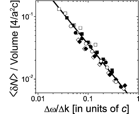
Fig. 2: Average absolute deviation of the calculated DOS from the exact total DOS $N(\omega)$ for an ‘empty crystal.’ The average runs over the frequency range $0<\omega<2\pi c/a$ and the deviation is in units of the DOS $N(\omega)$ per volume at $\omega\,a/2\pi c=1$, i.e., in units $4/a^{2}c$. In accordance with Eq. (19), the error is inversely proportional to the ratio $\Delta\omega/\Delta k$ of the histogram bin width $\Delta\omega$ to the integration grid spacing $\Delta k$. Symbols correspond to integration using the number of k-points $N_{k}$ = 280, 770, 1300, 2480, 2992 and 3570 ($\square,\blacksquare,\circ,\bullet,\lozenge,\blacklozenge$) respectively, with various $\Delta\omega$.

Indeed, the useful frequency resolution $\Delta\omega$ of a histogram of the DOS and LDOS is limited by the resolution $\Delta k$ of the grid in $\mathbf{k}$ space to be

$$\Delta\omega\approx\Delta k|\nabla_{\mathbf{k}}\omega|,$$ (19)

as detailed in Ref. [42] for the electronic DOS. This criterion relates the separation between adjacent $\mathbf{k}$-grid points to their approximate frequency spacing via the group velocity. If histogram bins are chosen too narrow compared to the expected frequency spacing between contributions to the discretized LDOS integral, unphysical spikes appear in the approximation, especially in the limit of small $\omega$, where the group velocity $|\nabla_{\mathbf{k}}\omega|$ is usually largest. Apart from full gaps in the LDOS, photonic crystals also promise sharp lines at which the LDOS is enhanced, which are important for non-classical emission dynamics. Hence it is especially important to distinguish sharp spikes that are due to histogram binning noise from true features. Unfortunately, many reports in literature feature sharp spikes that are evidently binning noise (wave vector undersampling errors), as they occur in the long wavelength limit, below any stop gap.

To improve the resolution without adding time-consuming diagonalizations, several interpolation schemes have been suggested [42]. Within the histogramming approach, an interpolation scheme essentially improves binning statistics by adding histogram contributions from intermediate grid points on the assumption that quantities vary linearly between grid points. While interpolation decouples the binning noise from the frequency bin width $\Delta\omega$, resulting in arbitrarily smooth LDOS approximations, it has the disadvantage of obscuring the intrinsic relation between frequency resolution and wave vector resolution in Eq. (19).

A good benchmark for the binning noise of the $\mathbf{k}$-space integration, independent of the convergence of the plane-wave method, is to calculate the LDOS or DOS of an ‘empty’ crystal, with uniform dielectric constant equal to unity. Such an ‘empty’ crystal represents a limit of zero photonic strength and the maximum possible group velocity $|\nabla_{\mathbf{k}}\omega|$. In Figure 1 we show the DOS in an empty fcc crystal. As expected for a crystal with zero dielectric contrast, the calculated DOS is independent of dipole position and orientation. In agreement with the well-known DOS in vacuum the calculated DOS increases parabolically with frequency. Fluctuations around the parabola are due to binning noise associated with the finite k-space discretization.

We have calculated the relative root-mean-square error in the calculated density of states (DOS) for an fcc ‘empty’ crystal averaged over all histogram bins in the frequency range $0<\omega a/2\pi c<1$ for several combinations of histogram binwidth and k-grid resolution, as specified in the caption of Fig. 2. As predicted by Eq. (19), the deviation of the approximation from the analytic result is inversely proportional to the ratio $\Delta\omega/\Delta k$. In most cases, one wants to calculate the LDOS with a given frequency resolution $\Delta\omega$, i.e. $N(\mathbf{r},\omega,\mathbf{e}_{d})\Delta\omega$, to within a predetermined accuracy. For instance, calculating the vacuum DOS for frequencies $0<\omega a/2\pi c<1$ with a desired absolute accuracy better than $0.01\cdot 4/a^{2}c$ (1% of the vacuum DOS at $\omega a/2\pi c=1$) and a desired frequency resolution of $\Delta\omega=0.01(2\pi c/a)$, requires using $\Delta k\sim\Delta\omega/0.3c$. The number of k-points corresponding to this wave vector sampling equals 2480 k-points in the irreducible wedge of the fcc Brillouin zone, 59520 in the required half Brillouin zone, or equivalently $N_{k}=119040$ in the full Brillouin zone. Photonic crystals with nonzero index contrast cause a pronounced frequency structure of the LDOS. Due to the flattening of bands compared to the dispersion bands of vacuum-only crystals, the k-space integration itself is at least as accurate, assuming that the eigenfrequencies and the field-mode patterns are known with infinite accuracy. In practice, one needs to adjust the number of plane waves to obtain all eigenfrequencies to within the desired frequency resolution $\Delta\omega$. In our computations for fcc crystals, we represented the k-space of a half of the first Brillouin zone by an equidistant grid consisting of $N_{k}/2=145708$ k-points. The frequency resolution of our LDOS histograms is $\Delta\omega=0.01\cdot 2\pi c/a$, and the spatial resolution of the LDOS is approximately $a/40$ judging from the maximum $|\mathbf{G}-\mathbf{G^{\prime}}|\approx 120/a$ involved in the expansion with $N_{G}$ = 725 plane waves in Eq. (4).

D Computation time required for LDOS

Calculating the LDOS in 3D periodic structures is a time-consuming task. The chosen degree of k-space discretization ($N_{k}/2=145708$ k-points) and the number of plane-waves ($N_{G}$ = 725) are the result of a trade-off between the desired accuracy and tolerated duration of the calculations. Essentially the computation consists of solving for the lowest $n$ eigenvalues and eigenvectors of a real symmetric $2N_{G}\times 2N_{G}$ matrix for each of the $N_{k}$ k-points independently. To accomplish this calculation, we use the standard Matlab ”eigs” implementation [43] of an implicitly restarted Arnoldi method (ARPACK) that takes approximately 2.2 seconds to find the lowest 20 eigenvalues and eigenvectors of a single Hermitian 1500x1500 (i.e., $N_{G}\approx 750$ plane waves) matrix on a 3 GHz Intel Pentium 4 processor, or on a 2.4 GHz Intel Core Duo processor. For $145708$ k-points the resulting computation time is hence on the order of 90 hours (4 days). Since the Matlab ARPACK routine is already highly optimized, we do not expect that the computation time per k-point can be significantly reduced for LDOS calculations based on the standard H-field inverted matrix plane wave method. In terms of the number of plane waves $N_{G}$, the computation time scales as $N_{G}^{3}$. As in Ref. [44], the algorithm can be accelerated by realizing that the iterative eigensolver does not require the full matrix ${\cal H}$ multiplying the vector $\mathbf{u}$ in Eq. LABEL:planewave3, but rather a function that quickly computes the image ${\cal H}\mathbf{u}$ of any trial vector $\mathbf{u}$. Since calculating ${\cal H}\mathbf{u}$ repeatedly involves a slow matrix-vector multiplication with $\eta_{\mathbf{G}-\mathbf{G^{\prime}}}$, the algorithm is only accelerated for $N_{G}>1000$.

3 Comparison with previous results

To test the computations, we compare our results with earlier reports. We have calculated the DOS and LDOS in an fcc crystal consisting of dielectric spheres with $\epsilon_{1}$ = 7.35 (TiO₂) in a medium with $\epsilon_{2}$ = 1.77 (water) – the same structure as was analyzed in Refs [31, 33]. The spheres occupy 25 vol% of the crystal. Figure 3 shows the total DOS in this photonic crystal calculated by us and by Busch and John [31] . We reproduce the earlier calculations of the total DOS: both results shown in Fig. 3 are in excellent agreement, with deviations less than 2% throughout the frequency range $0<\omega a/2\pi c<1$.

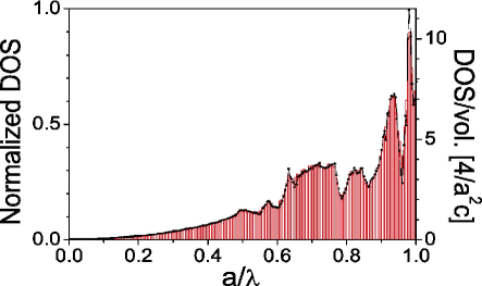
Fig. 3: (Color online)DOS per volume in an fcc crystal consisting of spheres with $\epsilon$ = 7.35 in a medium with $\epsilon$ = 1.77 with a filling fraction of the spheres of 25 vol %. The solid dotted curve represents calculations from Ref. [31]. Our result is plotted as a histogram (red).

In Figure 4 (Media 1)we demonstrate the LDOS in the same photonic crystal at a specific location: at a point equidistant from two nearest-neighbor spheres. In this calculation, we used the same number of reciprocal-lattice vectors N_G = 965 as in the only available benchmark paper by Wang et al. [33] that does not contain symmetry errors. We find that our calculations (empty circles) are in good agreement up to $a/\lambda=0.85$ with the LDOS reported previously (solid curve): the deviations are smaller than 1%. Deviations at higher frequencies are either due to a difference in accuracy of k-space integration (frequency binning resolution and k-space sampling density), or to a difference in accuracy of the plane wave methods (eigenmodes and eigenfrequencies).

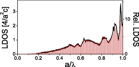
Fig. 4: (Color online) Dipole-averaged LDOS in the same photonic crystal as in Fig. 3 at a position $(\frac{1}{4},\frac{1}{4},0)$. Red histogram: our calculations (Media 1). Solid curve: results from Ref. [33]. This relative LDOS is the ratio of the LDOS to that in vacuum at $a/\lambda$ = 0.495.

Unfortunately, neither the accuracy nor the frequency resolution is specified in Ref. [33]. The k-space sampling density in our work is approximately twice the density specified in Ref. [33]. Based on the excellent agreement of our total DOS calculations with those of Busch and John [31], and on the fact that Wang et al. used a k-space density and plane wave number comparable to that of Busch and John, it is unlikely that inaccuracy of the k-space integration in either calculation is the source of discrepancy. We therefore surmise that deviations are due to a difference in the method of evaluation of $\mathbf{E}_{n,\mathbf{k}}(\mathbf{r})$. Conversion of $\mathbf{D}$ to $\mathbf{E}$ by multiplication with $1/\epsilon(\mathbf{r})$ in real space as proposed in [33] can cause incorrect mode amplitudes due to Gibbs oscillations, as opposed to the Fourier space conversion using Eq. (LABEL:eq:ecalcfromh). In general our calculations confirm the result by Wang et. al. [33] that the LDOS is only correctly calculated by integration over half the Brillouin zone, rather than over the irreducible part as was incorrectly used in earlier reports.

4 LDOS in TiO₂ inverse opals

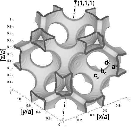
Fig. 5: Rendering of the dielectric function in one fcc unit cell that models the TiO₂ inverse-opal structure in section 4: an fcc lattice of air spheres of radius $r=0.25\sqrt{2}a$ with $a$ being the cubic lattice parameter. The spheres are covered by shells with $\epsilon=6.5$ and outer radius 1.09$r$. Neighboring air spheres are connected by windows of radius 0.4r. The letters (a–d) indicate four different positions at the TiO₂-air: a = $(1,0,0)/(2\sqrt{2})$, b = $(1,1,2)/(4\sqrt{3})$, c = $(1,1,1)/(2\sqrt{6})$ and d = (0.33,0.13,0) (points shown are symmetry-equivalents). The dash-dotted line shows the main diagonal of the cubic unit cell.

In recent time-resolved experiments, enhanced and inhibited emission rates were demonstrated for quantum dots embedded inside strongly photonic TiO₂ inverse opals [19, 21, 35]. In the framework of these experiments, it is highly relevant to calculate the LDOS inside such inverse-opal photonic crystals, especially for the source positions occupied in experiments. We model the position dependence of the dielectric function $\epsilon(\mathbf{r})$ as shown in Figure 5. This model assumes an infinite fcc lattice of air spheres with radius $r=0.25\sqrt{2}a$ (a is the cubic lattice parameter). The spheres are covered by overlapping dielectric shells ($\epsilon=6.5$) with outer radius 1.09r. Neighboring air spheres are connected by cylindrical windows of radius 0.4r. The resulting volume fraction of TiO₂ is equal to about 10.7%. These structural parameters are inferred from detailed characterization of the inverse opals using electron microscopy and small angle X-ray scattering [14, 15]. Moreover, the stop gaps in the photonic band structure (Fig. 6 (Media 2 and Media 3)) calculated using this model agree well with reflectivity measurements in the ranges of both the first-order ($a/\lambda=0.7$) and second-order Bragg diffraction ($a/\lambda=1.2$) [45].

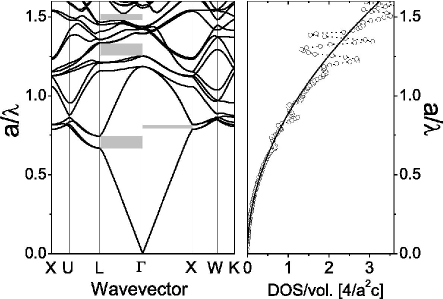
Fig. 6: Left: Photonic band structure (Media 2)for the TiO₂ inverse opal shown in Fig. 5. The grey rectangles indicate stopgaps in the $\Gamma$L direction and one stopgap in the $\Gamma$X direction for the inverse opal. The stopgaps result in the decreased DOS (right: circles, Media 3) at corresponding frequencies compared to the DOS in a homogeneous medium with $n_{av}=1.27$ (right: solid line).

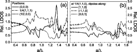
Fig. 7: Relative LDOS in the inverse opal shown in Fig 5 at three different positions: (a, Media 4) $\mathbf{r}$ = (0,0,0) [the center of an air sphere, solid curve], $\mathbf{r}$ = $\frac{1}{4}(1,1,1)$ [among three air spheres, dash-dotted curve] and $\mathbf{r}$ = ($\frac{1}{2}$,0,0) [midway between two spheres along [1,0,0] direction, dotted curve]; (b, Media 5) $\mathbf{r}$ = $\frac{1}{4}(1,1,0)$ [in the window between two spheres] projected on [1,1,0], [-1,1,0] and [0,0,1] directions shown by solid, dash-dotted and dotted curves, respectively.

Henceforth, we will consider the relative LDOS, which is the ratio of the LDOS in a photonic crystal to that in a homogeneous medium with the same volume-averaged dielectric function. This scaling is motivated by experimental practice, in which emission rate modifications are judged by normalizing measured rates to the emission rate of the same emitter in crystals with much smaller lattice constant $a$ [19, 21, 35]. In these reference systems, emission frequencies correspond to the effective medium limit $a/\lambda\ll 0.5$ quantified by an average index $n_{av}=\sqrt{\epsilon_{av}}=1.27$ for the TiO₂ crystals [19]. In units of $4/a^{2}c$, the LDOS in a homogeneous medium is equal to $n_{av}(a/\lambda)^{2}/3$. In Figure 7a (Media 4) we plot the resulting LDOS at three positions in the unit cell: at r = (0,0,0), $\frac{1}{4}(1,1,1)$ and ($\frac{1}{2}$,0,0). Due to the high symmetry of these points, the LDOS does not depend on the dipole orientation, as we verified explicitly. A first main observation from Fig. 7a (Media 4) is that the LDOS differs considerably between these three positions at all reduced frequencies. This observation illustrates the well-known strong dependence of the LDOS on position within the unit cell of photonic crystals [27, 10, 31].

A second main observation in Fig. 7a (Media 4) is that the LDOS strongly varies with reduced frequency, revealing troughs and peaks caused by the pseudogap near $a/\lambda=0.7$, which is related to $1^{st}$-order stop gaps such as the L-gap. The effects of $2^{nd}$-order stopgaps appear beyond $a/\lambda>1.15$ [45]. In the middle of the air region at position r = (0,0,0) there is a sharp, factor-of-three enhancement at $a/\lambda\approx 1.35$ within a narrow frequency range. This feature could be probed by resonant atoms infiltrated in the crystals [46]. At position r = ($\frac{1}{2}$,0,0) in an interstitial, the mode density has a broad trough near $a/\lambda=1.25$ that will lead to strongly inhibited emission.

A third main observation is that at spatial positions with low symmetry, the LDOS clearly depends on the orientation of the transition dipole moment. Figure 7b (Media 5) shows the frequency dependent LDOS for three perpendicular dipole orientations at a position in the center of a window that connects two neighboring air spheres (see Figure 5). The LDOS differs for all three orientations, and is thus anisotropic. At low frequency ($a/\lambda=0.3$), the emission rate is highest for a dipole pointing in the $(1,1,0)$ direction, with increasing frequency the highest rate shifts to the $(0,0,1)$ and then to the $(-1,1,0)$ orientation. We emphasize that for emitters with fixed or slowly varying dipole orientations, such as dye molecules or quantum dots on solid interfaces, the emission rate is determined by the optical modes that are projected on the dipole orientation. Therefore, knowledge of the projected LDOS is important for controlling spontaneous-emission rates as well as for interpreting the data from experiments on emitters in photonic metamaterials.

A fourth main observation from Fig. 7a and b (Media 4 and 5) is that at low frequencies $a/\lambda<0.5$, the relative LDOS hardly varies with frequency, which means that the mode density is proportional to $\omega^{2}$, as in homogeneous media. Interestingly, there is a clear dependence of the LDOS on both the position and the dipole orientation even at these low frequencies, i.e., long wavelengths relative to the crystal periodicity. The reason for these effects is that the photonic Bloch modes exhibit local variations of the electric field related to local variations of the dielectric function in order to satisfy the continuity equations at dielectric boundaries for the parallel $\mathbf{E}$ or perpendicular $\mathbf{D}$ field, respectively [34, 47]. Consequently, the LDOS strongly varies on length scales much less than the wavelength, i.e., even in electrostatic or effective medium limit. While such behavior may appear surprising, its origin in electrostatic depolarization effects has been discussed before [48, 47].

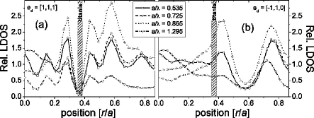
Fig. 8: Relative LDOS at four key frequencies, $a/\lambda$ = 0.535, 0.725, 0.865 and 1.295, in the inverse opal as a function of position r from (0,0,0) in the [1,1,1] direction. The hatched boxes indicate the position of the dielectric TiO₂ shell. The LDOS is projected on two dipole orientations: (a) [1,1,1] perpendicular to the dielectric-air interface, and (b) [-1,1,0] parallel to the interface. The LDOS projected on the [-1,-1,2] and [-1,1,0] directions is equal. For $r/a\in[\frac{\sqrt{3}}{2},\sqrt{3}]$ the LDOS is mirror-symmetric to that in the region [$0,\frac{\sqrt{3}}{2}]$.

To gain more insight in the spatial dependence of the LDOS in the inverse opals, we have performed calculations for dipoles positioned along a characteristic axis in the unit cell. Figure 8 shows the LDOS at four key frequencies for dipoles placed on the body diagonal of the cubic unit cell, that is, from $(0,0,0)$ in the $[1,1,1]$ direction. The LDOS has clear maxima and minima along the diagonal, varying by more than $10\times$. Figure 8(a) shows that for a dipole oriented in the $[1,1,1]$ direction (perpendicular to the dielectric-air interface), the LDOS is strongly ($>$ 5x) suppressed near the dielectric TiO₂ shell ($\emph{r/a}\approx 0.353$) at all frequencies. In contrast, no strong suppression or enhancement occurs for dipole orientations parallel to the dielectric interface, see Fig. 8(b). The strongly differing LDOS for dipoles near the dielectric rationalize the broad distributions of emission rates that were recently observed for quantum dots in inverse opals [35], see below. Enhancements and inhibitions also occur in the air regions: the LDOS is enhanced at $\emph{r/a}\approx$ 0.28 and 0.57 by up to 2.5 to 3 times, respectively, see Figure 8(a). At point $\emph{r/a}=1/\sqrt{3}\approx 0.57$ that lies in the (111) lattice plane in the air region, the LDOS is inhibited at all frequencies for the dipole orientations [-1,1,0] and [-1,-1,2] that are perpendicular to the (111) plane (see Fig. 8(b)). Finally, for dipoles parallel to the body diagonal (Figure 8(a)) the mode density shows pseudo-oscillatory behavior on length scales much less than the wavelength, e.g., a period of $0.2a$ at frequency $0.535a/\lambda$ (period corresponds to $1/10^{th}$ of a wavelength). This observation confirms that photonic crystals are bona fide metamaterials where optical properties strongly vary on length scales much less than the wavelength.

Fig. 9: Relative LDOS in the inverse opal at four different positions on the TiO₂-air interface shown in Fig. 5. At each position the LDOS is projected on three mutually orthogonal dipole orientations $\mathbf{e}_{d}$. (a, Media 6) point a for $\mathbf{e}_{d}$ = [1,0,0] and [0,1,0]. LDOS at $\mathbf{e}_{d}$ = [0,0,1] and [0,1,0] is the same. (b, Media 7) point b for $\mathbf{e}_{d}$ = [1,1,2], [-1,1,0] and [-1,-1,1]. (c, Media 8) point c for $\mathbf{e}_{d}$ = [1,1,1] and [-1,1,0]. LDOS at $\mathbf{e}_{d}$ = [-1,-1,2] is equal to that at $\mathbf{e}_{d}$ = [-1,1,0]. (d, Media 9) point d for $\mathbf{e}_{d}$ = [0.33,0.13,0], [-0.13,0,0.33] and [0,0,1].

In recent time-resolved experiments [21, 35], emission from quantum dot light sources distributed at the internal TiO₂-air interfaces of the inverse opals was investigated. To analyze the experimental data, we have calculated the LDOS at several symmetry-inequivalent positions on the TiO₂ shells: at points a, b, c and d (see Fig. 5) for three mutually orthogonal orientations of the emitting dipole, where the first orientation is chosen along the vector pointing from (0,0,0) toward the corresponding point. Figures 9(a) through 9(d) (Media 6 through 9) show that at all these positions the LDOS strongly varies with reduced frequency and position, as expected, and also with orientation of the dipole. In broad terms, for a dipole parallel to the interface the LDOS is near 1 at low frequency, increases to a peak enhancement of $2.5\times$ at $a/\lambda=1.22$ before strongly varying at high frequencies. For reference, the frequency $a/\lambda=1.22$ is in the range where a band gap is expected for more strongly interacting crystals. The plots also reveal that for dipoles perpendicular to the TiO₂-air interface, the LDOS is strongly inhibited (more than $10\times$) over broad frequency ranges. For instance, Figure 9(a) shows that the emission rate for a dipole perpendicular to the interface is 16-fold inhibited to a level of 0.06, with a maximum of 0.22 (5-fold inhibition) at $a/\lambda=1.22$. It is striking that the strong inhibition occurs over a broad frequency range from 0.3 to 1.6, i.e., more than two octaves in frequency. While the inhibition is not complete, the bandwidth is much larger than the maximum bandwidth of $12\%$ for a full 3D bandgap in inverse opals[49] and far exceeds the bandwidth of the 2D gap for TE modes in membrane photonic crystals, that allows a seven-fold inhibition [30, 26] over a 30% bandwidth.

In the frequency range up to $a/\lambda=1.1$, the dependence of the LDOS on frequency is quite similar at all the positions and dipole orientations. This remarkable result agrees with the experimental observation from Ref. [35]: the complex decay curves of light sources in the inverse opals are described by one and the same functional shape (log-normal) of the decay-rate distribution for all reduced frequencies studied.

For the interpretation of the time-resolved experiments on ensembles of emitters in the inverse-opal photonic crystals, the results presented above mean that

1. the decay rate of an individual emitter is determined by its frequency, position and also by the orientation of its transition dipole in the photonic crystal;

2. the measured spontaneous-emission decay depends on how the emitters are distributed in the crystal;

3. even in the low-frequency regime, ensemble measurements will reveal non-exponentional decay curves;

4. the similar shape of the reduced-frequency dependence of the LDOS allows modeling of the non-exponentional decay curves with a single type of decay-rate distributions. In other words, one distribution function can be successfully used to model the multi-exponentional decay curves measured from crystals with different lattice parameters.

5 LDOS in silicon inverse opals

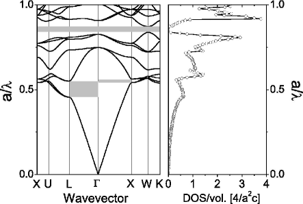
Fig. 10: Left: Photonic band structure (Media 10) for an inverse opal from silicon ($\epsilon$ = 11.9). Right: The total DOS in the Si inverse opal (Media 11). The DOS is strongly depleted for frequencies near $\Gamma$L and $\Gamma$X stopgaps (grey rectangles). A photonic band gap (grey bar) occurs between bands 8 and 9, as also reflected in the vanishing DOS.

A complete inhibtion of spontaneous emission may only be achieved in photonic crystals with a 3D photonic band gap. Therefore, there has been much effort to fabricate inverse opals from silicon rather than titania, since the higher index of silicon allows for a photonic band gap [31, 37]. For the calculation of the LDOS in such Si inverse opals, the dielectric function $\epsilon(\mathbf{r})$ was modeled similarly to that in the inverse opals shown in Fig. 5. From SEM observations we inferred the following structural parameters [17, 18]: the outer radius of the overlapping dielectric shells with $\epsilon=11.9$ is about 1.15r (where $r=0.25\sqrt{2}a$ is the air-sphere radius, a is the lattice parameter). The cylindrical windows connecting neighboring air spheres have a radius of 0.2r. The larger outer radius and the smaller window size compared to the TiO₂ inverse opals are commensurate with a higher volume fraction of about 23% Si [18].

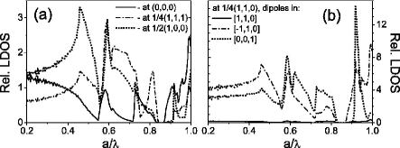
Fig. 11: Relative LDOS in a Si inverse opal at: (a, Media 12) $\mathbf{r}$ = (0,0,0) [the center of an air sphere, solid curve], $\mathbf{r}$ = $\frac{1}{4}(1,1,1)$ [among three air spheres, dash-dotted curve] and $\mathbf{r}$ = ($\frac{1}{2}$,0,0) [midway between two spheres along [1,0,0] direction, dotted curve]; (b, Media 13) $\mathbf{r}$ = $\frac{1}{4}(1,1,0)$ [in the window between two air spheres] projected on [1,1,0], [-1,1,0] and [0,0,1] directions shown by solid, dash-dotted and dotted curves, respectively.

The band structure and total DOS for this system are shown in Fig. 10 (Media 10 and Media 11). The DOS is strongly depleted in a pseudo-gap between the $2^{nd}$ and $3^{rd}$ bands [36], at frequencies near 0.55. Near frequency 0.85, both the band structures and the DOS reveal a 3D photonic band gap of relative width $\Delta\omega/\omega\approx 3~{}\%$ between the $8^{th}$ and $9^{th}$ bands [31]. Compared to the TiO₂ structure, both the lowest-order L-gap and the $8^{th}$ and $9^{th}$ bands are shifted to lower reduced frequencies. This shift is due to the higher effective refractive index of the Si inverse opals ($n_{av}=1.88$), on account of a higher index of the backbone and a higher filling fraction.

Figure 11(a) (Media 12) presents the relative LDOS at three high-symmetry positions in the unit cell r = (0,0,0), $\frac{1}{4}(1,1,1)$ and $(\frac{1}{2},0,0)$. The LDOS varies much more strongly with frequency than in TiO₂ inverse opals, as a result of the larger dielectric contrast that leads to strongly modified dispersion relations and Bloch mode profiles. While the maxima up to 3.2 are not much higher than in TiO₂ inverse opals, the minima in the mode density are reduced and the slopes are steeper. As expected, the LDOS is completely inhibited at all positions in the frequency range of the band gap. Previously, it has been suggested that the LDOS could be inhibited at salient positions in the unit cell for frequencies outside a complete gap. While Figure 11(a) (Media 12) reveals that the mode density is strongly reduced above the band gap, e.g., at $\mathbf{r}=(\frac{1}{2},0,0)$, it is not truly inhibited. In fact, in the course of our study, we have not encountered any ”sweet spots” where the LDOS is completely inhibited at frequencies outside a 3D photonic band gap.

Figure 11(b) (Media 13) shows the LDOS at a lower symmetry position r = $\frac{1}{4}(1,1,0)$, in the window between two nearest-neighbor air spheres. The mode density has been calculated for three perpendicular dipole orientations. Figure 11(b) (Media 13) shows that the LDOS is highly anisotropic since it differs for all three orientations: at low frequencies ($a/\lambda<0.5$), the mode density is highest for the $(-1,1,0)$ orientation, intermediate for the $(0,0,1)$ orientation, and lowest for the $(1,1,0)$ orientation. With increasing frequency, the highest LDOS also changes to other orientations, with the $(0,0,1)$ orientation having the highest LDOS above the pseudo-gap and even a narrow peak at frequency 0.95. Therefore, if it is possible to orient a quantum emitter with its dipole parallel to $(0,0,1)$, this frequency range is conducive to strong emission enhancement and perhaps even QED effects beyond weak-coupling. Interestingly, these frequencies are slightly higher than the upper edge of the band gap where strong coupling effects have recently been discussed [12].

6 Conclusions

We have performed intensive calculations of the local density of states in TiO₂ and Si inverse opals with experimentally relevant structural parameters. Since conflicting and incorrect reports have appeared on the LDOS in photonic crystals, we have set out to validate our method of choice, i.e., the H-field plane-wave expansion method. This validation relied on comparison to literature results, on the explicit verification of required symmetries that previous reports failed to satisfy, and on quantitative considerations of resolution and accuracy. Results for each structure are made available for other workers in the field, both as benchmarks and for comparison with experimental data. With the help of these computations we have obtained quantitative insight in the LDOS relevant for time-resolved ensemble fluorescence measurements on photonic crystals, such as obtained in recent experimental work [35]. The results of our numerical calculations reveal a surprisingly strong dependence of the LDOS on the orientation of the emitting dipoles.

References

- [1] J. D. Joannopoulos, S. G. Johnson, J.N. Winn and R. D. Meade, Photonic Crystals: Molding the Flow of Light, 2nd edition, (Princeton University Press, 2008).
- [2] C. M. Soukoulis, editor, Photonic Crystals and Light Localization in the Century, (Kluwer, Dordrecht 2001).
- [3] V. P. Bykov, “Spontaneous emission in a periodic structure,” Sov. Phys. JETP 35, 269-273 (1972).
- [4] “Spontaneous emission from a medium with a band spectrum,” Sov. J. Quant. Electron. 4, 861-871 (1975).
- [5] E. Yablonovitch, “Inhibited spontaneous emission in solid-state physics and electronics,” Phys. Rev. Lett. 58, 2059-2062 (1987).
- [6] S. John, “Strong localization of photons in certain disordered dielectric superlattices,” Phys. Rev. Lett. 58, 2486-2489 (1987).
- [7] O. Painter, R. K. Lee, A. Scherer, A. Yariv, J. D. O’Brien, P. D. Dapkus and I. Kim,“Two-dimensional photonic band-gap defect mode laser,” Science 284, 1819 1821 (1999).
- [8] H.-G. Park, S.-H. Kim, S.-H. Kwon, Y.-G. Ju, J.-K. Yang, J.-H. Baek, S.-B. Kim, Y.-H. Lee, “Electrically driven single-cell photonic crystal laser,” Science, 305, 1444-1447 (2004).
- [9] M. Grätzel, “Photoelectrochemical cells,” Nature 414, 338-344 (2001).
- [10] R. Sprik, B.A. van Tiggelen, and A. Lagendijk, “Optical emission in periodic dielectrics,” Europhys. Lett. 35, 265-270 (1996).
- [11] N. Vats, S. John and K. Busch, “Theory of fluorescence in photonic crystals,” Phys. Rev. A 65, 043808 (2002).
- [12] P. Kristensen, A. F. Koenderink, P. Lodahl, B. Tromborg, and J. Mørk, “Fractional decay of quantum dots in real photonic crystals,” Opt. Lett. 33, 1557-1559 (2008).
- [13] K. Busch, S. Lölkes, R. B. Wehrspohn and H. Föll, editors, Photonic Crystals. Advances in Design, Fabrication, and Characterization,(Wiley-VCH Verlag GmbH & Co., Weinheim 2004).
- [14] J.E.G.J. Wijnhoven and W. L. Vos, “Preparation of photonic crystals made of air spheres in titania,” Science 281, 802-804, (1998).
- [15] J.E.G.J. Wijnhoven, L. Bechger and W. L. Vos, “Fabrication and characterization of large macroporous photonic crystals in titania,” Chem. Mater. 13, 4486-4499 (2001).
- [16] A. A. Zakhidov, R. H. Baughman, Z. Iqbal, C. Cui, I. Khayrullin, S. O. Dantas, J. Marti, and V. G. Ralchenko, “Carbon structures with three-dimensional periodicity at optical wavelengths,” Science 282, 897-901 (1998).
- [17] A. Blanco, E. Chomski, S. Grabtchak, M. Ibisate, S. John, S. W. Leonard, C. López, F. Meseguer, H. Míguez, J. P. Mondia, G. A. Ozin, O. Toader, and H. M. van Driel, “Large-scale synthesis of a silicon photonic crystal with a complete three-dimensional bandgap near 1.5 micrometres,” Nature 405, 437-440 (2000).
- [18] Y. A. Vlasov, X. Z. Bo, J. C. Sturm, and D. J. Norris, “On-chip natural assembly of silicon photonic bandgap crystals,” Nature 414, 289-293 (2001).
- [19] A.F. Koenderink, L. Bechger, H. P. Schriemer, A. Lagendijk and W. L. Vos, “Broadband fivefold reduction of vacuum fluctuations probed by dyes in photonic crystals,” Phys. Rev. Lett. 88, 143903 (2002).
- [20] S. Ogawa, M. Imada, S. Yoshimoto, M. Okato and S. Noda, “Control of light emission by 3D photonic crystals,” Science 305, 227-229 (2004).
- [21] P. Lodahl, A. F. van Driel, I. S. Nikolaev, A. Irman, K. Overgaag, D. Vanmaekelbergh, and W. L. Vos, “Controlling the dynamics of spontaneous emission from quantum dots by photonic crystals,” Nature 430, 654 (2004).
- [22] A. Badolato, K. Hennessy, M. Atatüre, J. Dreiser, E. Hu, P. M. Petroff, A. Imamoğlu, “Deterministic coupling of single quantum dots to single nanocavity modes,” Science 308, 1158-1161 (2005).
- [23] A. Kress, F. Hofbauer, N. Reinelt, M. Kaniber, H. J. Krenner, R. Meyer, G. Böhm, and J. J. Finley, “Manipulation of the spontaneous emission dynamics of quantum dots in two-dimensional photonic crystals,” Phys. Rev. B 71, 241304 (2005).
- [24] M. Fujita, S. Takahashi, Y. Tanaka, T. Asano, S. Noda, “Simultaneous inhibition and redistribution of spontaneous light emission in photonic crystals,” Science 308, 1296-1298 (2005).
- [25] D. Englund, D. Fattal, E. Waks, G. Solomon, B. Zhang, T. Nakaoka, Y. Arakawa, Y. Yamamoto, J. Vuc̆ković, “Controlling the spontaneous emission rate of single quantum dots in a two-Dimensional photonic crystal,” Phys. Rev. Lett. 95, 013904 (2005).
- [26] B. Julsgaard, J. Johansen, S. Stobbe, T. Stolberg-Rohr, T. Sünner, M. Kamp, A. Forchel and P. Lodahl, “Decay dynamics of quantum dots influenced by the local density of optical states in two-dimensional photonic crystal membranes,” Appl. Phys. Lett. 93, 094102 (2008).
- [27] T. Suzuki and P. K. L. Yu, “Emission power of an electric dipole in the photonic band structure of the fcc lattice,” J. Opt. Soc. Am. B 12, 570-582 (1995).
- [28] R. K. Lee, Y. Xu, A. Yariv, “Modified spontaneous emission from a two-dimensional photonic bandgap crystal slab,” J. Opt. Soc. Am. B 17, 1438–1442 (2000).
- [29] C. Hermann and O. Hess, “Modified spontaneous emission rate in an inverted-opal structure with complete photonic bandgap,” J. Opt. Soc. Am. B 19, 3013–3018 (2002).
- [30] A. F. Koenderink, M. Kafesaki, C.M. Soukoulis and V. Sandoghdar, “Spontaneous emission control in two-dimensional photonic crystal membranes,” J. Opt. Soc. Am. B 23, 1196-1206 (2006).
- [31] K. Busch and S. John, “Photonic band gap formation in certain self-organizing systems”, Phys. Rev. E 58, 3896-3908 (1998).
- [32] Z.-Y. Li, L.-L. Lin, and Z.-Q. Zhang, “Spontaneous emission from photonic crystals: full vectorial calculations,” Phys. Rev. Lett. 84, 4341 (2000).
- [33] R. Wang, X.-H. Wang, B.-Y. Gu and G.-Z. Yang, “Local density of states in three-dimensional photonic crystals: calculation and enhancement effects,” Phys. Rev. B 67, 155114 (2003).
- [34] D. P. Fussell, R. C. McPhedran, and C. M. de Sterke, “Three-dimensional Green’s tensor, local density of states, and spontaneous emission in finite two-dimensional photonic crystals composed of cylinders,”, Phys. Rev. E 70, 066608 (2004).
- [35] I. S. Nikolaev, P. Lodahl, A. F. van Driel, A. F. Koenderink, and W. L. Vos, “Strongly nonexponential time-resolved fluorescence of quantum-dot ensembles in three-dimensional photonic crystals,” Phys. Rev. B 75, 115302 (2007).
- [36] K. M. Ho, C. T. Chan and C. M. Soukoulis, “Existence of a photonic gap in periodic dielectric structures”, Phys. Rev. Lett. 65, 3152-3155 (1990).
- [37] H.S. Sözüer, J.W. Haus, and R. Inguva, “Photonic bands: convergence problems with the plane-wave method,” Phys. Rev. B 45, 13962 (1992).
- [38] J.D. Jackson, Classical Electrodynamics, (John Wiley & Sons, New York 1975).
- [39] N. W. Ashcroft and N. D. Mermin, Solid State Physics, (Holt, Rinehart and Winston, New York, 1976).
- [40] L. Li, “Use of Fourier series in the analysis of discontinuous periodic structures,” J. Opt. Soc. Am. A 13, 1870-1876 (1996).
- [41] H. J. Monkhorst and J. D. Pack, “Special points for Brillouin-zone integration,” Phys. Rev. B 13, 5188-5192 (1976).
- [42] G. Gilat, “Analysis of methods for calculating spectral properties in solids,” J. Comput. Phys. 10, 432-465 (1972).
- [43] R. B. Lehoucq, D. C. Sorensen, and C. Yang, ARPACK User s Guide: Solution of Large-Scale Eigenvalue Problems with Implicitly Restarted Arnoldi Methods, (SIAM Publications, Philadelphia 1998).
- [44] S. G. Johnson and J. D. Joannopoulos, “Block-iterative frequency-domain methods for Maxwell’s equations in a planewave basis,” Opt. Express 8, 173-190 (2001).
- [45] W. L. Vos and H. M. van Driel, “Higher order Bragg diffraction by strongly photonic fcc crystals: onset of a photonic bandgap,” Phys. Lett. A 272, 101 (2000).
- [46] P.J. Harding, Photonic crystals modified by optically resonant systems, (Ph.D. thesis, University of Twente (2008). ISBN 978-90-365-2683-8, available from www.photonicbandgaps.com
- [47] L. Rogobete, H. Schniepp, V. Sandoghdar and C. Henkel, “Spontaneous emission in nanoscopic dielectric particles,” Opt. Lett. 28, 1736-1738 (2003).
- [48] H. Miyazaki and K. Ohtaka, Phys. Rev. B 58, 6920 (1998).
- [49] A.F. Koenderink, Emission and transport of light in photonic crystals, (Ph.D. thesis, University of Amsterdam (2003)). ISBN 90-9016903-2, available from www.photonicbandgaps.com