Energy scales and magnetoresistance at a quantum critical point

Abstract

The magnetoresistance (MR) of $\rm CeCoIn_{5}$ is notably different from that in many conventional metals. We show that a pronounced crossover from negative to positive MR at elevated temperatures and fixed magnetic fields is determined by the scaling behavior of quasiparticle effective mass. At a quantum critical point (QCP) this dependence generates kinks (crossover points from fast to slow growth) in thermodynamic characteristics (like specific heat, magnetization etc) at some temperatures when a strongly correlated electron system transits from the magnetic field induced Landau Fermi liquid (LFL) regime to the non-Fermi liquid (NFL) one taking place at rising temperatures. We show that the above kink-like peculiarity separates two distinct energy scales in QCP vicinity - low temperature LFL scale and high temperature one related to NFL regime. Our comprehensive theoretical analysis of experimental data permits to reveal for the first time new MR and kinks scaling behavior as well as to identify the physical reasons for above energy scales.

I Introduction

An explanation of rich and striking behavior of strongly correlated electron system in heavy fermion (HF) metals is, as years before, among the main problems of condensed matter physics. One of the most interesting and puzzling issues in the research of HF metals is their anomalous normal-state transport properties. Measurements of magnetoresistance (MR) on $\rm{CeCoIn_{5}}$pag ; mal have shown that it is notably different from ordinary weak-field orbital MR described by Kohler’s rule which holds in many conventional metals, see e.g. zim . At fixed magnetic fields $B$, MR of $\rm CeCoIn_{5}$ exhibits a crossover from negative (low temperatures) to positive (hight temperatures) one at temperature growth pag ; mal . This crossover is hard to explain within both conventional Fermi liquid approach for metals and in terms of Kondo systems daybell . To explain this effect, it has been assumed that the crossover can be attributed to some distinct energy scales revealed by kinks (crossover points from fast to slow growth) in thermodynamic characteristics (like specific heat, magnetization etc) and leading to a change of spin fluctuations character with increasing of the applied magnetic field strength pag ; mal ; daybell ; loh ; si ; steg ; kon ; nak .

Here we investigate the NFL-LFL transition region (we call it below crossover region), where MR changes its sign. The modified Kohler’s rule (MR versus tangent of Hall angle) have been utilized to describe MR data kon ; nak . In this region, both Kohler’s rule and its modified version do not work. In Landau Fermi liquid (LFL) regime, the quasiparticles were observed in measurements of transport properties in $\rm CeCoIn_{5}$ pag1 . An analysis of above thermodynamic quantities shows that quasiparticles exist in both LFL and crossover regimes when strongly correlated Fermi systems like HF metals or two-dimensional (2D) $\rm{}^{3}He$ ckz ; obz ; shag1 ; shag2 ; shag3 ; khodb transit from LFL to NFL behavior. It is of crucial importance to verify whether quasiparticles with effective mass $M^{*}$ still exist and determine the transport properties and energy scales in HF metals in crossover region. On the other hand, even early measurements on HF metals gave evidences in favor of the quasiparticles existence. For example, the application of magnetic field $B$ restores LFL behavior of HF metals which demonstrate NFL properties in the absence of the field . In that case the empirical Kadowaki-Woods (KW) ratio $K$ is conserved, $K=A(B)/\gamma_{0}^{2}(B)\propto A(B)/\chi^{2}(B)=const$ kadw ; kh_z ; tky where $\gamma_{0}=C/T$, $C$ is a heat capacity, $\chi$ is a magnetic susceptibility and $A(B)$ is a coefficient determining the temperature dependence of the resistivity $\rho=\rho_{0}+A(B)T^{2}$. Here $\rho_{0}$ is the residual resistance. The observed conservation of $K$ can be hardly interpreted within scenarios when quasiparticles are suppressed, for there is no reason to expect that $\gamma_{0}(B)$, $\chi(T)$, $A(B)$ and other transport and thermodynamic quantities like thermal expansion coefficient $\alpha(B)$ are affected by the fluctuations or localization in a correlated fashion. As we will see below, the MR measurements in the crossover region can present indicative data on the quasiparticles availability. Such MR measurements were carried out in $\rm{CeCoIn_{5}}$ when the system transits from LFL to NFL regime at elevated temperatures and fixed magnetic fields pag ; mal .

In this Letter, we analyze MR of $\rm{CeCoIn_{5}}$ and show that the crossover from negative to positive MR at elevated temperatures and fixed magnetic fields can be well captured utilizing fermion condensation quantum phase transition (FCQPT) concept based on the quasiparticles paradigm khs ; obz ; ams ; volovik . We demonstrate that the crossover is regulated by the universal behavior of the effective mass $M^{*}(B,T)$ observed in many HF metals. It is exhibited by $M^{*}(B,T)$ when HF metal transits from LFL regime (induced by the application of magnetic field) to NFL one taking place at rising temperatures. The above behavior of the effective mass also generates kinks (crossover points from fast to slow growth at elevated temperatures) in thermodynamic characteristics (like specific heat, magnetization etc). We show that the above kink-like peculiarity separates two distinct energy scales - low temperature LFL scale and high temperature one related to NFL regime. Our calculations of MR are in good agreement with observations and allow us to reveal new scaling behavior of both MR and the kinks.

II Scaling behavior of the kinks

To study universal low temperature features of HF metals, we use the model of homogeneous heavy-fermion liquid with the effective mass $M^{*}(T,B,x)$, where $x=p_{F}^{3}/3\pi^{2}$ is a number density and $p_{F}$ is Fermi momentum land . This model permits to avoid complications associated with the crystalline anisotropy of solids shag1 . We first outline the case when at $T\to 0$ the heavy-electron liquid behaves as LFL and is brought to the LFL side of FCQPT by tuning of a control parameter like $x$. At elevated temperatures the system transits to the NFL state. The dependence $M^{*}(T,x)$ is governed by Landau equation land

$$\frac{1}{M^{*}(T,x)}=\frac{1}{M}+\int\frac{{\bf p}_{F}{\bf p}}{p_{F}^{3}}F({\bf p_{F}},{\bf p})\frac{\partial n({\bf p},T,x)}{\partial{p}}\frac{d{\bf p}}{(2\pi)^{3}},$$ (1)

where $n({\bf p},T,x)$ is the distribution function of quasiparticles and $F({\bf p}_{F},{\bf p})$ is Landau interaction amplitude, $M$ is a free electron mass. At $T=0$, eq. (1) reads land $M^{*}/M=1/(1-N_{0}F^{1}(p_{F},p_{F})/3)$. Here $N_{0}$ is the density of states of a free electron gas, $F^{1}(p_{F},p_{F})$ is the $p$-wave component of Landau interaction amplitude $F$. Taking into account that $x=p_{F}^{3}/3\pi^{2}$, we rewrite the amplitude as $F^{1}(p_{F},p_{F})=F^{1}(x)$. When at some critical point $x=x_{FC}$, $F^{1}(x)$ achieves certain threshold value, the denominator tends to zero and the system undergoes FCQPT related to divergency of the effective mass khs ; volovik ; obz ; khodb ,

$$\frac{M^{*}(x)}{M}=A+\frac{B}{x_{FC}-x}.$$ (2)

Equation (2) is valid in both 3D and 2D cases, while the values of factors $A$ and $B$ depend on the dimensionality. The approximate solution of Eq. (1) is of the form shag2

$$\frac{M}{{M^{*}(T)}} = \frac{M}{{M^{*}(x)}}+\beta f(0)\ln\left\{{1+\exp(-1/\beta)}\right\}$$ (3)

$$+ \lambda_{1}\beta^{2}+\lambda_{2}\beta^{4}+...,$$

where $\lambda_{1}>0$ and $\lambda_{2}<0$ are constants of order unity, $\beta=TM^{*}(T)/p_{F}^{2}$ and $f(0)\sim F^{1}(x_{FC})$. It follows from Eq. (3) that the effective mass $M^{*}$ as a function of $T$ and $x$ reveals three different regimes at growing temperature. At the lowest temperatures we have LFL regime with $M^{*}(T,x)\simeq M^{*}(x)+aT^{2}$ with $a<0$ since $\lambda_{1}>0$. The effective mass as a function of $T$ decays down to a minimum and after grows, reaching its maximum $M^{*}_{M}$ at some temperature $T_{M}(x)$ then subsequently diminishing as $T^{-2/3}$ ckz ; obz . Moreover, the closer is the number density $x$ to its threshold value $x_{FC}$, the higher is the rate of the growth. The peak value $M^{*}_{M}$ grows also, but the maximum temperature $T_{M}$ lowers. Near this temperature the last ”traces” of LFL regime disappear, manifesting themselves in the divergence of above low-temperature series and substantial growth of $M^{*}(x)$. Numerical calculations based on Eqs. (1) and (3) show that at rising temperatures $T>T_{1/2}$ ($T_{1/2}$ is a characteristic temperature determining the validity of regime (4), see Ref. shag2 for details) the linear term $\propto\beta$ gives the main contribution and leads to new regime when Eq. (3) reads $M/M^{*}(T)\propto\beta$ yielding

$$M^{*}(T)\propto T^{-1/2}.$$ (4)

We remark that Eq. (4) ensures that at $T\geq T_{1/2}$ the resistivity behaves as $\rho(T)\propto T$ obz .

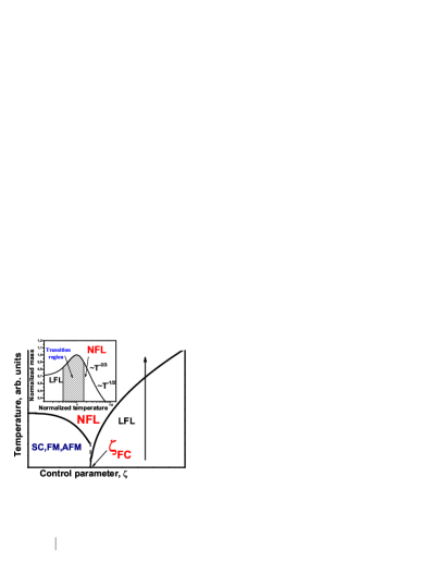
Figure 1: Schematic phase diagram of the systems under consideration. Control parameter $\zeta$ represents number density (or doping) $x$, magnetic field $B$, pressure $P$ etc. $\zeta_{\rm FC}$ denotes the point of effective mass divergence. $\rm{SC,FM,AFM}$ denote the superconducting, ferromagnetic and antiferromagnetic states, respectively. The vertical arrow shows LFL-NFL transitions at rising temperatures and fixed $\zeta$. Inset shows a schematic plot of the normalized effective mass $M^{*}_{N}=M^{*}(T/T_{M})/M^{*}_{M}$ ($M^{*}_{M}$ is its maximal value at $T=T_{M}$) versus the normalized temperature $T_{N}=T/T_{M}$. Several regions are shown. First goes the LFL regime ($M^{*}_{N}(T_{N})\sim$ const) at $T_{N}\ll 1$, then the transition regime (the hatched area) where $M^{*}_{N}$ reaches its maximum. At elevated temperatures $T^{-2/3}$ regime occurs followed by $T^{-1/2}$ behavior, see Eq. (4).

Near the critical point $x_{FC}$ ($M/M^{*}(x\to x_{FC})\to 0$), the behavior of the effective mass changes dramatically since the first term in the right-hand side of Eq. (3) vanishes so that the second term becomes dominant. As a result, we can no more measure the mass $M^{*}$ in units of $M$ (as $M/M^{*}(x\to x_{FC})\to 0$) and we have to measure $M^{*}$ in units of $M^{*}_{M}$ and $T$ in units of $T_{M}$. Latter scales can be viewed as natural ones.

The schematic phase diagram of HF liquid is reported Fig. 1. The control parameter $\zeta$ can be pressure $P$, magnetic field $B$, or doping (density) $x$. At $\zeta=\zeta_{FC}$, FCQPT takes place leading to a strongly degenerated state. This state is captured by the superconducting (SC), ferromagnetic (FM), antiferromagnetic (AFM) etc. states lifting the degeneracy obz . The variation of $\zeta$ drives the system from NFL region to LFL one. For example, in the case of magnetic field $B$, $\zeta_{FC}=B_{c0}$, where $B_{c0}$ is a critical magnetic field, such that at $B>B_{c0}$ the system is driven towards its LFL regime. Below we consider the case with $\zeta>\zeta_{FC}$ when the system is on the LFL side of FCQPT. The inset demonstrates the behavior of the normalized effective mass $M^{*}_{N}=M^{*}/M^{*}_{M}$ versus normalized temperature $T_{N}=T/T_{M}$. Both $T^{-2/3}$ and $T^{-1/2}$ regimes are marked as NFL ones since the effective mass depends strongly on temperature. The temperature region $T\simeq T_{M}$ signifies the crossover between the LFL regime with almost constant effective mass and NFL behavior, given by $T^{-2/3}$ dependence. Thus temperatures $T\sim T_{M}$ can be regarded as the crossover region between LFL and NFL regimes.

It turns out that $M^{*}(T,x)$ in the entire $T\leq T_{1/2}$ range can be well approximated by a simple universal interpolating function obz ; shag2 ; ckz . The interpolation occurs between the LFL ($M^{*}\propto T^{2}$) and NFL ($M^{*}\propto T^{-1/2}$, see Eq. (4)) regimes thus describing the above crossover. Introducing the dimensionless variable $y=T_{N}=T/T_{M}$, we obtain the desired expression

$$\frac{M^{*}(T/T_{M},x)}{M^{*}_{M}}={M^{*}_{N}(y)}\approx\frac{M^{*}(x)}{M^{*}_{M}}\frac{1+c_{1}y^{2}}{1+c_{2}y^{8/3}}.$$ (5)

Here $M^{*}_{N}(y)$ is the normalized effective mass, $c_{1}$ and $c_{2}$ are parameters, obtained from the condition of best fit to experiment. To correct the behavior of $M^{*}_{N}(y)$ at rising temperatures $M^{*}\sim T^{-1/2}$, we add a term to Eq. (5) and obtain

$$M^{*}_{N}(y)\approx\frac{M^{*}(x)}{M^{*}_{M}}\left[\frac{1+c_{1}y^{2}}{1+c_{2}y^{8/3}}+c_{3}\frac{\exp(-1/y)}{\sqrt{y}}\right],$$ (6)

where $c_{3}$ is a parameter. The last term on the right hand side of Eq. (6) makes $M^{*}_{N}$ satisfy Eq. (4) at temperatures $T/T_{M}>2$.

At small magnetic fields $B$ (that means that Zeeman splitting is small), the effective mass does not depend on spin variable and $B$ enters Eq. (1) as $B\mu_{B}/T$ ($\mu_{B}$ is Bohr magneton) making $T_{M}\propto B\mu_{B}$ ckz ; obz ; shag2 . The application of magnetic field restores the LFL behavior, and at $T\leq T_{M}$ the effective mass depends on $B$ as ckz ; obz

$$M^{*}(B)\propto(B-B_{c0})^{-2/3}.$$ (7)

Note that in some cases $B_{c0}=0$. For example, the HF metal $\rm{CeRu_{2}Si_{2}}$is characterized by $B_{c0}=0$ and shows neither evidence of the magnetic ordering or superconductivity nor the LFL behavior down to the lowest temperatures takah . In our simple model $B_{c0}$ is taken as a parameter. We conclude that under the application of magnetic field the variable

$$y=T/T_{M}\propto\frac{T}{\mu_{B}(B-B_{c0})}$$ (8)

remains the same and the normalized effective mass is again governed by Eqs. (5) and (6) which are the final result of our analytical calculations. We note that the obtained results are in agreement with numerical calculations obz ; ckz .

The normalized effective mass $M^{*}_{N}(y)$ can be extracted from experiments on HF metals. For example, $M^{*}(T,B)\propto C(T)/T\propto S(T)/T\propto\chi_{AC}(T)$, where $S(T)$ is the entropy, $C(T)$ is the specific heat and $\chi_{AC}(T)$ is ac magnetic susceptibility ckz ; obz . If the corresponding measurements are carried out at fixed magnetic field $B$ (or at fixed $x$ and $B$) then, as it seen from Fig. 1, the effective mass reaches the maximum at some temperature $T_{M}$. Upon normalizing both the effective mass by its peak value $M^{*}_{M}$ at each field $B$ and the temperature by $T_{M}$, we observe that all the curves merge into a single one, given by Eqs. (5) and (6) thus demonstrating a scaling behavior.

To verify Eq. (4), we use measurements of $\chi_{AC}(T)$ in $\rm{CeRu_{2}Si_{2}}$ at $B=0.02$ mT at which this HF metal demonstrates the NFL behavior takah . It is seen from Fig. 2 that Eq. (4) gives good description of the facts in the extremely wide range of temperatures. The inset to Fig. 2 exhibits a fit for $M^{*}_{N}(y)$ extracted from measurements of $\chi_{AC}(T)$ at different magnetic fields, clearly indicating that the function given by Eq. (5) represents a good approximation for $M^{*}_{N}(y)$ when the system transits from the LFL regime to NFL one.

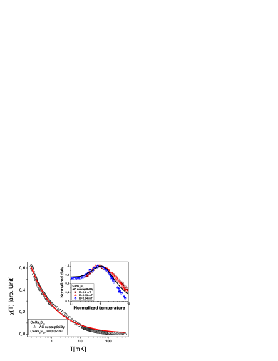
Figure 2: Temperature dependence of the $ac$ susceptibility $\chi_{AC}$ for $\rm{CeRu_{2}Si_{2}}$. The solid curve is a fit for the data shown by the triangles at $B=0.02$ mT and represented by the function $\chi(T)=a/\sqrt{T}$ given by Eq. (4) with $a$ being a fitting parameter. Inset shows the normalized effective mass versus normalized temperature $y$ extracted from $\chi_{AC}$ measured at different fields as indicated in the inset takah . The solid curve traces the universal behavior of $M^{*}_{N}(y)$ determined by Eq. (5). Parameters $c_{1}$ and $c_{2}$ are adjusted to fit the average behavior of the normalized effective mass $M^{*}_{N}(y)$.

$M^{*}_{N}(y)$ extracted from the entropy $S(T)/T$ and magnetization $M$ measurements on the ³He film he3 at different densities $x$ is reported in the left panel of Fig. 3. In the same panel, the data extracted from the heat capacity of the ferromagnet $\rm{CePd_{0.2}Rh_{0.8}}$ pikul and the AC magnetic susceptibility of the paramagnet $\rm{CeRu_{2}Si_{2}}$ takah are plotted for different magnetic fields. It is seen that the universal behavior of the normalized effective mass given by Eq. (5) and shown by the solid curve is in accord with the experimental facts. All 2D $\rm{{}^{3}He}$ substances are located at $\zeta>\zeta_{FC}$ (see Fig. 1), where the system progressively disrupts its LFL behavior at elevated temperatures. In that case the control parameter, driving the system towards its quantum critical point (QCP) is merely the number density $x$. It is seen that the behavior of $M^{*}_{N}(y)$, extracted from $S(T)/T$ and magnetization $M$ of 2D $\rm{{}^{3}He}$ looks very much like that of 3D HF compounds. In the right panel of Fig. 3, the normalized data on $C(y)$, $S(y)$, $y\chi(y)$ and $M(y)+y\chi(y)$ extracted from data collected on $\rm{CePd_{1-x}Rh_{x}}$ pikul , $\rm{{}^{3}He}$ he3 , $\rm{CeRu_{2}Si_{2}}$ takah , $\rm CeCoIn_{5}$ bian and $\rm{YbRu_{2}Si_{2}}$ steg respectively are presented. Note that in the case of $\rm{YbRu_{2}Si_{2}}$, the variable $y=(B-B_{c0})\mu_{B}/T_{M}$ can be viewed as effective normalized temperature. As seen from Eq. (5), this representation of the variable $y$ is correct when the temperature is a fixed parameter.

It is seen from the right panel of Fig. 3 that all the data exhibit the kink (shown by arrow) at $y\geq 1$ taking place as soon as the system enters the transition region from the LFL regime to the NFL one and corresponding to the temperatures where the vertical arrow in Fig. 1 crosses the solid line. It is also seen that the low temperature LFL scale of the thermodynamic functions (as a function of $y$) is characterized by the fast growth and the high temperature one related to the NFL behavior is characterized by the slow growth. As a result, we can identify the energy scales near QCP, discovered in Ref. steg : the thermodynamic characteristics exhibit the kinks (crossover points from the fast to slow growth at elevated temperatures) which separate the low temperature LFL scale and high temperature one related to NFL regime.

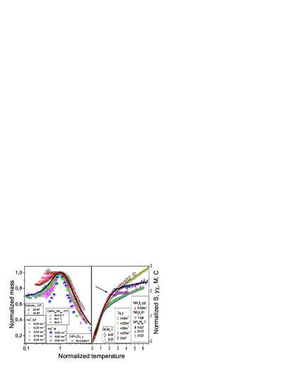
Figure 3: The left panel. The normalized effective mass $M^{*}_{N}$ versus the normalized temperature $y=T/T_{M}$. The dependence $M^{*}_{N}(y)$ is extracted from measurements of $S(T)/T$ and magnetization $M$ on 2D $\rm{{}^{3}He}$ he3 ), from $ac$ susceptibility $\chi_{AC}(T)$ collected on $\rm{CeRu_{2}Si_{2}}$ takah and from $C(T)/T$ collected on $\rm{CePd_{1-x}Rh_{x}}$ pikul . The data are collected for different densities and magnetic fields shown in the left bottom corner. The solid curve traces the universal behavior of the normalized effective mass determined by Eq. (5). Parameters $c_{1}$ and $c_{2}$ are adjusted for $\chi_{N}(T_{N},B)$ at $B=0.94$ mT. The right panel. The normalized specific heat $C(y)$ of $\rm{CePd_{1-x}Rh_{x}}$ at different magnetic fields $B$, normalized entropy $S(y)$ of $\rm{{}^{3}He}$ at different number densities $x$, and the normalized $y\chi(y)$ at $B=0.94$ mT versus normalized temperature $y$ are shown. The upright triangles depict the normalized ‘average’ magnetization $M+B\chi$ collected on $\rm{YbRu_{2}Si_{2}}$ steg . The kink (shown by the arrow) in all the data is clearly seen in the transition region $y\geq 1$. The solid curve represents $yM^{*}_{N}(y)$ with parameters $c_{1}$ and $c_{2}$ adjusted for magnetic susceptibility of $\rm{CeRu_{2}Si_{2}}$ at $B=0.94$ mT.

III Scaling behavior of the magnetoresistance

By definition, MR is given by

$$\rho_{mr}(B,T)=\frac{\rho(B,T)-\rho(0,T)}{\rho(0,T)},$$ (9)

We apply Eq. (9) to study MR of strongly correlated electron liquid versus temperature $T$ as a function of magnetic field $B$. The resistivity $\rho(B,T)$ is

$$\rho(B,T)=\rho_{0}+\Delta\rho(B,T)+\Delta\rho_{L}(B,T),$$ (10)

where $\rho_{0}$ is a residual resistance, $\Delta\rho=c_{1}AT^{2}$, $c_{1}$ is a constant, $A$ is a coefficient determining the temperature dependence of the resistivity $\rho=\rho_{0}+AT^{2}$. The classical contribution $\Delta\rho_{L}(B,T)$ to MR due to orbital motion of carriers induced by the Lorentz force obeys the Kohler’s rule zim . We note that $\Delta\rho_{L}(B)$ $\ll\rho(0,T)$ as it is assumed in the weak-field approximation. To calculate $A$, we use the quantities $\gamma_{0}=C/T\propto M^{*}$ and/or $\chi\propto M^{*}$ as well as employ the fact that Kadowaki-Woods ratio $K=A/\gamma_{0}^{2}\propto A/\chi^{2}=const$ kadw . As a result, we obtain $A\propto(M^{*})^{2}$ kadw ; kh_z ; tky , so that $\Delta\rho(B,T)=c(M^{*}(B,T))^{2}T^{2}$ and $c$ is a constant. Suppose that the temperature is not very low, so that $\rho_{0}\leq\Delta\rho(B=0,T)$, and $B\geq B_{c0}$. Substituting (10) into (9), we find that shag_mr

$$\rho_{mr}\simeq\frac{\Delta\rho_{L}}{\rho}+cT^{2}\frac{(M^{*}(B,T))^{2}-(M^{*}(0,T))^{2}}{\rho(0,T)}.$$ (11)

Consider the qualitative behavior of MR described by Eq. (11) as a function of $B$ at a certain temperature $T=T_{0}$. In weak magnetic fields, when $T_{0}\geq T_{1/2}$ and the system exhibits NFL regime (see Fig. 1), the main contribution to MR is made by the term $\Delta\rho_{L}(B)$, because the effective mass is independent of the applied magnetic field. Hence, $|M^{*}(B,T)-M^{*}(0,T)|/M^{*}(0,T)\ll 1$ and the leading contribution is made by $\Delta\rho_{L}(B)$. As a result, MR is an increasing function of $B$. When $B$ becomes so high that $T_{M}(B)\sim\mu_{B}(B-B_{c0})\sim T_{0}$, the difference $(M^{*}(B,T)-M^{*}(0,T))$ becomes negative and MR as a function of $B$ reaches its maximal value at $T_{M}(B)\sim T_{0}$ when the kink occurs, see the right panel of Fig. 3. At further increase of magnetic field, when $T_{M}(B)>T_{0}$, the effective mass $M^{*}(B,T)$ becomes a decreasing function of $B$, as follows from Eq. (7). As $B$ increases,

$$\frac{(M^{*}(B,T)-M^{*}(0,T))}{M^{*}(0,T)}\to-1,$$ (12)

and the magnetoresistance, being a decreasing function of $B$, is negative.

Now we study the behavior of MR as a function of $T$ at fixed value $B_{0}$ of magnetic field. At low temperatures $T\ll T_{M}(B_{0})$, it follows from Eqs. (5) and (7) that $M^{*}(B_{0},T)/M^{*}(0,T)\ll 1$, and it is seen from Eq. (12) that $\rho_{mr}(B_{0},T)\sim-1$, because $\Delta\rho_{L}(B_{0},T)/\rho(0,T)\ll 1$. We note that $B_{0}$ must be relatively high to guarantee that $M^{*}(B_{0},T)/M^{*}(0,T)$ $\ll 1$. As the temperature increases, MR increases, remaining negative. At $T\simeq T_{M}(B_{0})$, MR is approximately zero, because $\rho(B_{0},T)\simeq\rho(0,T)$ at this point. This allows us to conclude that the change of the temperature dependence of resistivity $\rho(B_{0},T)$ from quadratic to linear manifests itself in the transition from negative to positive MR. One can also say that the transition takes place when the kink occurs (as shown by the arrow in the right panel of Fig. 3) and the system goes from the LFL behavior to the NFL one. At $T\geq T_{M}(B_{0})$, the leading contribution to MR is made by $\Delta\rho_{L}(B_{0},T)$ and MR reaches its maximum. At $T_{M}(B_{0})\ll T$, MR is a decreasing function of the temperature, because

$$\frac{|M^{*}(B,T)-M^{*}(0,T)|}{M^{*}(0,T)}\ll 1,$$ (13)

and $\rho_{mr}(B_{0},T)\ll 1$. Both transitions (from positive to negative MR with increasing $B$ at fixed temperature $T$ and from negative to positive MR with increasing $T$ at fixed $B$ value) have been detected in measurements of the resistivity of $\rm{CeCoIn_{5}}$ in a magnetic field pag .

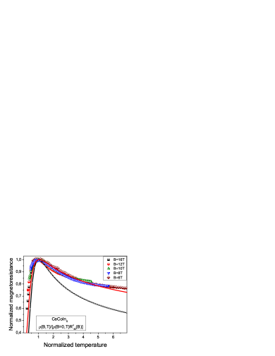
Figure 4: The normalized magnetoresistance $R^{\rho}_{N}(y)$ given by Eq. (15) versus normalized temperature $y=T/T_{\rm Rm}$. $R^{\rho}_{N}(y)$ was extracted from MR shown in Fig. 6 and collected on $\rm{CeCoIn_{5}}$ at fixed magnetic fields $B$ pag listed in the right upper corner. The starred line represents our calculations based on Eqs. (5) and (15) with the parameters extracted from $ac$ susceptibility of $\rm CeRu_{2}Si_{2}$ (see the caption to Fig. 2). The solid line displays our calculations based on Eqs. (6) and (15); only one parameter was used to fit the data, while the other were extracted from the $ac$ susceptibility measured on $\rm{CeRu_{2}Si_{2}}$.

Let us turn to quantitative analysis of MR. As it was mentioned above, we can safely assume that the classical contribution $\Delta\rho_{L}(B,T)$ to MR is small as compared to $\Delta\rho(B,T)$. Omission of $\Delta\rho_{L}(B,T)$ allows us to make our analysis and results transparent and simple since the behavior of $\Delta\rho_{L}(B_{0},T)$ is not known in the case of HF metals. Consider the ratio $R^{\rho}=\rho(B,T)/\rho(0,T)$ and assume for a while that the residual resistance $\rho_{0}$ is small in comparison with the temperature dependent terms. Taking into account Eq. (10) and $\rho(0,T)\propto T$, we obtain from Eq. (11)

$$R^{\rho}=\rho_{mr}+1=\frac{\rho(B,T)}{\rho(0,T)}\propto T(M^{*}(B,T))^{2}.$$ (14)

It follows from Eqs. (5) and (14) that the ratio $R^{\rho}$ reaches its maximal value $R^{\rho}_{M}$ at some temperature $T_{\rm Rm}\sim T_{M}$. If the ratio is measured in units of its maximal value $R^{\rho}_{M}$ and $T$ is measured in units of $T_{\rm Rm}\sim T_{M}$ then it is seen from Eqs. (5), (6) and (14) that the normalized MR

$$R^{\rho}_{N}(y)=\frac{R^{\rho}(B,T)}{R^{\rho}_{M}(B)}\simeq y(M^{*}_{N}(y))^{2}$$ (15)

becomes a universal function of the only variable $y=T/T_{\rm Rm}$. To verify Eq. (15), we use MR obtained in measurements on CeCoIn₅, see Fig. 1(b) of Ref. pag . The results of the normalization procedure of MR are reported in Fig. 4. It is clearly seen that the data collapse into the same curve, indicating that the normalized magnetoresistance $R^{\rho}_{N}$ well obeys the scaling behavior given by Eq. (15). This scaling behavior obtained directly from the experimental facts is a vivid evidence that MR behavior is predominantly governed by the effective mass $M^{*}(B,T)$.

Now we are in position to calculate $R^{\rho}_{N}(y)$ given by Eq. (15). Using Eq. (5) to parameterize $M^{*}_{N}(y)$, we extract parameters $c_{1}$ and $c_{2}$ from measurements of the magnetic $ac$ susceptibility $\chi$ on $\rm CeRu_{2}Si_{2}$ takah and apply Eq. (15) to calculate the normalized ratio. It is seen that the calculations shown by the starred line in Fig. 4 start to deviate from experimental points at elevated temperatures. To improve the coincidence, we employ Eq. (6) which describes the behavior of the effective mass at elevated temperatures in accord with Eq. (4) and ensures that at these temperatures the resistance behaves as $\rho(T)\propto T$. In Fig. 4, the fit of $R^{\rho}_{N}(y)$ by Eq. (6) is shown by the solid line. Constant $c_{3}$ is taken as a fitting parameter, while the other were extracted from $ac$ susceptibility of $\rm{CeRu_{2}Si_{2}}$ as described in the caption to Fig. 2.

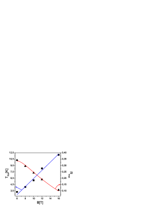
Figure 5: The peak temperatures $T_{\rm Rm}$ (squares) and the peak values $R_{\rm max}$ (triangles) versus magnetic field $B$ extracted from measurements of MR pag . The solid lines represent our calculations based on Eqs. (16) and (17).

Before discussing the magnetoresistance $\rho_{mr}(B,T)$ given by Eq. (9), we consider the magnetic field dependencies of both the MR peak value $R_{\rm max}(B)$ and corresponding peak temperature $T_{\rm Rm}(B)$. It is possible to use Eq. (14) which relates the position and value of the peak with the function $M^{*}(B,T)$. Since $T_{\rm Rm}\propto\mu_{B}B$, $B$ enters Eq. (14) only as tuning parameter of QCP, as both $\Delta\rho_{L}$ and $\rho_{0}$ were omitted. At $B\to B_{c0}$ and $T\leq T_{\rm Rm}(B)$, this omission is not correct since $\Delta\rho_{L}$ and $\rho_{0}$ become comparable with $\Delta\rho(B,T)$. Therefore, both $R_{\rm max}(B)$ and $T_{\rm Rm}(B)$ are not characterized by any critical field, being a continuous function at the quantum critical filed $B_{c0}$, in contrast to $M^{*}(B,T)$ which peak value diverges and the peak temperature tends to zero at $B_{c0}$ as it follows from Eqs. (7) and (8). Thus, we have to take into account $\Delta\rho_{L}(B,T)$ and $\rho_{0}$ which prevent $T_{\rm Rm}(B)$ from vanishing and make $R_{\rm max}(B)$ finite at $B\to B_{c0}$. As a result, we have to replace $B_{c0}$ by some effective field $B_{eff}<B_{c0}$ and take $B_{eff}$ as a parameter which imitates the contributions coming from both $\Delta\rho_{L}(B,T)$ and $\rho_{0}$. Upon modifying Eq. (14) by taking into account $\Delta\rho_{L}(B,T)$ and $\rho_{0}$, we obtain

$$T_{\rm Rm}(B)\simeq b_{1}(B-B_{eff}),$$ (16)

$$R_{\rm max}(B)\simeq\frac{b_{2}(B-B_{eff})^{-1/3}-1}{b_{3}(B-B_{eff})^{-1}+1}.$$ (17)

Here $b_{1}$, $b_{2}$, $b_{3}$ and $B_{eff}$ are fitting parameters. It is pertinent to note that while deriving Eq. (17) we use Eq. (16) with substitution $(B-B_{eff})$ for $T$. Then, Eqs. (16) and (17) are not valid at $B\lesssim B_{c0}$. In Fig. 5, we show the field dependence of both $T_{\rm Rm}$ and $R_{\rm max}$, extracted from measurements of MR pag . It is seen that both $T_{\rm Rm}$ and $R_{\rm max}$ are well described by Eqs. (16) and (17) with $B_{eff}=$3.8 T. We note that this value of $B_{eff}$ is in good agreement with observations obtained from the $B-T$ phase diagram of $\rm{CeCoIn_{5}}$, see the position of the MR maximum shown by the filled circles in Fig. 3 of Ref. pag .

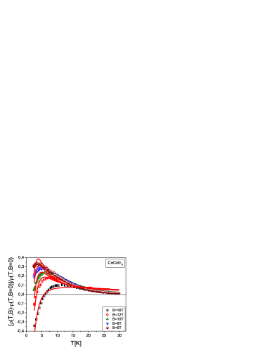
Figure 6: MR versus temperature $T$ as a function of magnetic field $B$. The experimental data on MR were collected on $\rm{CeCoIn_{5}}$ at fixed magnetic field $B$ pag shown in the right bottom corner of the Figure. The solid lines represent our calculations, Eq. (5) is used to fit the effective mass entering Eq. (15).

To calculate $\rho_{mr}(B,T)$, we apply Eq. (15) to describe its universal behavior, Eq. (5) for the effective mass along with Eqs. (16) and (17) for MR parameters. Figure 6 shows the calculated MR versus temperature as a function of magnetic field $B$ together with the experimental points from Ref. pag . We recall that the contributions coming from $\Delta\rho_{L}(B,T)$ and $\rho_{0}$ were omitted. As seen from Fig. 6, our description of experiment is pretty good.

IV Summary

Our comprehensive theoretical study of MR shows that it is (similar to other thermodynamic characteristics like magnetic susceptibility, specific heat etc) governed by the scaling behavior of the quasiparticle effective mass. The crossover from negative to positive MR occurs at elevated temperatures and fixed magnetic fields when the system transits from the LFL behavior to NFL one and can be well captured by this scaling behavior. This behavior permits to identify the energy scales near QCP, discovered in Ref. steg . Namely, the thermodynamic characteristics (like specific heat, magnetization etc) consist of the low temperature LFL scale characterized by the fast growth and the high temperature one related to the NFL behavior and characterized by the slow growth. These scales are separated by the kinks in the transition region. Obtained theoretical results are in good agreement with experimental facts and allow us to reveal for the first time a new scaling behavior of both magnetoresistance and kinks separating the different energy scales.

V Acknowledgements

This work was supported in part by the grants: RFBR No. 09-02-00056, DOE and NSF No. DMR-0705328, and the Hebrew University Intramural Funds.

References

- (1) J. Paglione, et. al., Phys. Rev. Lett. 91 (2003) 246405.
- (2) A. Malinowski, et. al., Phys. Rev. B72 (2005) 184506.
- (3) J. M. Ziman, Electrons and Phonons, Oxford University Press, Oxford, 1960.
- (4) M. D. Daybell, W. A. Steyert, Phys. Rev. Lett. 18 (1967) 398.
- (5) H.v. Löhneysen, A. Rosch, M. Vojta, P. Wölfle, Rev. Mod. Phys. 79 (2007) 1015.
- (6) P. Gegenwart, Q. Si, F. Steglich, Nature Phys. 4 (2008) 186.
- (7) P. Gegenwart, et. al., Science 315 (2007) 969.
- (8) H. Kontani, Rep. Prog. Phys. 71 (2008) 026501.
- (9) Y. Nakajima, et. al., Journ. Phys. Soc. Japan 76 (2007) 024703.
- (10) J. Paglione, et. al., Phys. Rev. Lett. 97 (2006) 106606.
- (11) J.W. Clark, V.A. Khodel, M.V. Zverev Phys. Rev. B71 (2005) 012401.
- (12) V.R. Shaginyan, M.Ya. Amusia, K.G. Popov, Physics-Uspekhi 50 (2007) 563.
- (13) V.R. Shaginyan, et. al., Europhys. Lett. 76 (2006) 898.
- (14) V.R. Shaginyan, K.G. Popov, V.A. Stephanovich, Europhys. Lett. 79 (2007) 47001.
- (15) V.R. Shaginyan, et. al., Phys. Rev. Lett. 100 (2008) 096406.
- (16) V.A. Khodel, J.W. Clark, M.V. Zverev, Phys. Rev. B78 (2008) 075120.
- (17) K. Kadowaki, S.B. Woods, Solid State Commun. 58 (1986) 507.
- (18) V.A. Khodel, P. Schuck, Z. Phys. B 104 (1997) 505.
- (19) N. Tsujii, H. Kontani, K. Yoshimura, Phys. Rev. Lett. 94 (2005) 057201.
- (20) V.A. Khodel, V.R. Shaginyan, JETP Lett. 51 (1990) 553.
- (21) M. Ya. Amusia, V.R. Shaginyan, Phys. Rev. B63 (2001) 224507.
- (22) G.E. Volovik, Springer Lecture Notes in Physics 718 (2007) 31.
- (23) L.D. Landau, Sov. Phys. JETP 3 (1956) 920.
- (24) D. Takahashi, et al., Phys. Rev. B67 (2003) 180407(R).
- (25) M. Neumann, J. Nyéki, J. Saunders, Science 317 (2007) 1356.
- (26) A.P. Pikul, et al., J. Phys. Condens. Matter 18 (2006) L535.
- (27) A. Bianchi, et. al., Phys. Rev. Lett. 91 (2003) 257001.
- (28) V.R. Shaginyan, JETP Lett. 77 (2003) 178.