Analyzing SN 2003Z with PHOENIX

Abstract

Aims. We present synthetic spectra around maximum for the type II supernova SN 2003Z, which was first detected on January 29.7 2003. Comparison with observed spectra aim at the determination of physical parameters for SN 2003Z.

Methods. Synthetic spectra are calculated with our stellar atmosphere code PHOENIX. It solves the special relativistic equation of radiative transfer, including large NLTE-calculations and line blanketing by design, in 1-dimensional spherical symmetry. The observed spectra were obtained at the 3.5 meter telescope at Calar Alto. The TWIN instrument was used so that a spectral range from about 3600 to 7500 Å was covered. The spectra were taken on Feb. 4, 5, 9, and 11, 2003.

Results. The physical parameters of the models give the luminosities, a range of possible velocity profiles for the SN, an estimate of the colour excess, and the observed metalicity.

1 Introduction

Type II supernovae (SNe II) are thought to originate from the core collapse of massive stars. By definition SNe II show strong Balmer lines in their spectra, and thus are thought to be from stars with much of their hydrogen envelopes intact at the time of the explosion. Largely through the use of HST, progenitors have been identified for several SNe II, and they seem to come from rather low mass stars $9\mathrel{\hbox{\hbox to0.0pt{\hbox{\lower 4.0pt\hbox{$\sim$}}\hss}\hbox{$>$}}}M\mathrel{\hbox{\hbox to0.0pt{\hbox{\lower 4.0pt\hbox{$\sim$}}\hss}\hbox{$<$}}}12$ ${\mbox{M}_{\odot}}$ (Maund et al. 2005; Maund & Smartt 2005; Smartt et al. 2003, 2004; Van Dyk et al. 2003a, b, c).

Since the spectra of SNe II form in hydrogen dominated atmospheres with relatively simple density structures, they should be among the most accurate spectra to model with detailed model atmosphere codes.

Indeed, SNe II can be modeled in detail and reddening, primordial metalicity, and even distances can be determined (Baron et al. 2000, 2003, 2004). Thus, through detailed spectral modeling we can determine important physical parameters that can be compared with stellar evolution and explosion modeling.

Here, we use the PHOENIX relativistic model atmosphere code package (Hauschildt & Baron 1999; Hauschildt et al. 1997; Baron & Hauschildt 1998; Hauschildt et al. 2001) to simulate the SN II atmosphere for SN 2003Z during its optically thick (photospheric) phase.

In the following we first describe the observations of SN 2003Z, and then describe our modeling process including the assumptions made to construct a model. After that we present our results about luminosities, extinction, velocity profiles. Finally the results are summarized in the conclusion.

2 The supernova SN 2003Z

SN 2003Z was discovered on January 29, 2003 (Boles et al. 2003) and is a type II supernova (Matheson et al. 2003).

The SN was observed on the 4th, 5th, 9th, and 11th of February 2003 with the 3.5 meter telescope at Calar Alto. The TWIN spectrograph was used, covering the spectral range from about 3600 to 7400 Å. The SN is located near the galaxy NGC 2742 and is believed to lie in the outer part of a spiral arm of the galaxy, typical for a Type II supernova. The redshift of NGC 2742 is $z=0.0043$ (Falco et al. 1999).

From NED the foreground colour excess of the galaxy is $E(B-V)=0.039$ (Schlegel et al. 1998). Information about the radial velocity of the SN itself or the colour excess of the host galaxy are unavailable.

The physical structure of the atmosphere changes over time due to the expansion and the gradual cooling of the ejected material. Therefore, the spectrum also changes over time. From day to day the changes are small; however, the spectra of the first and the last day of the observations show large differences as displayed in Fig. 1.

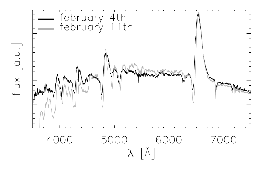
Figure 1: Comparison of the spectra of the first and last day of the observations. A shift in wavelength towards the red and a decrease of flux in the blue part are visible, indicating the cooling and slowing of the material producing the spectra.

The gradual change in the wavelength shift of the spectral lines originates from the changing optical depth of the cooling and expanding envelope. As time progresses we see into slower and “deeper” layers of the atmosphere so that the lines show smaller redshifts in the later spectra.

3 Modeling

PHOENIX is a general purpose NLTE stellar atmosphere code package. For the calculation of the radiative transfer with PHOENIX the structure of the atmosphere is approximated by a spherically symmetric shell, thereby reducing the system to one spatial dimension. Furthermore, the envelope is assumed to be homologously expanding, giving a linearly increasing velocity field (Sedov solution)

$$v(r)=v_{0}\frac{r}{R_{0}}$$ (1)

with $v_{0}$ being the velocity and $R_{0}$ the radius at $\tau=1$ in the radial optical depth grid. The run of the density is approximated by a power law (Zel’dovich & Raizer 1967)

$$\rho(r) = \left(\frac{r}{R_{0}}\right)^{-n}$$ (2)

Due to the fact that the atmosphere of a SN is expanding at $\simeq 10$ percent of the speed of light, the special relativistic equation (Mihalas & Weibel Mihalas 1984) of radiative transfer in moving media must be solved. In co-moving form written in terms of wavelengths we have

$$\eta_{\lambda}-\chi_{\lambda}I_{\lambda} = \frac{\partial I_{\lambda}}{\partial s}+a_{\lambda}\frac{\partial\lambda I_{\lambda}}{\partial\lambda}+4a_{\lambda}I_{\lambda}$$ (3)

$${\rm with:}\quad a_{\lambda} = \gamma\left[\frac{\beta(1-\mu^{\prime 2})}{r}+\gamma^{2}\mu^{\prime}(\mu^{\prime}+\beta)\frac{\partial\beta}{\partial r}\right]$$

where $I_{\lambda}$ is the specific intensity and the differentiation of the path-length $s$ is the differentiation along the monochromatic path of a photon in the co-moving frame. Furthermore, $\eta_{\lambda}$ is the emissivity and $\chi_{\lambda}$ the extinction coefficient. The emissivity $\eta$ depends via scattering on the mean intensity $J_{\lambda}$ itself, therefore, the problem is not a mere differential equation but an integro-differential equation. The radiative transfer problem is solved with an operator splitting technique in the co-moving frame (Hauschildt & Baron 2004; Hauschildt 1992). For the NLTE models, the coupled radiation transport and rate equation problem is solved by a multi-level operator splitting method (Hauschildt 1993).

Details of the code and the numerical methods used in PHOENIX can be found in Hauschildt & Baron (1999).

All models were calculated on a radial grid with 100 layers, using a logarithmic optical depth grid ($\tau$-grid) in the continuum at 5000 Å with a range from $\tau=10^{3}-10^{-10}$.

Other model parameters vary from model to model. For instance the final model for the first day of the observation had a pressure at $\tau=1$ of $4.44\cdot 10^{-8}$ bar and the corresponding radius was $9.62\cdot 10^{14}$ cm.

Unstable nuclei – most importantly $\@element[56]{\mathrm{Ni}}$ – are created in SN outburst and, therefore, the input of radioactive energy plays an important role in the formation of the spectrum. The treatment of the influence of radioactivity is simplified by the assumption that $\gamma$-ray deposition follows the density profile and the total mass of radiative nuclei is a parameter in the modeling. In all models we iterated the temperature structure to fulfill the condition of energy conservation in the co-moving frame. Furthermore, the most important species were treated in complete NLTE. (see Table  1). The decision which ionization stages were included in NLTE was made by taking into account the partial pressures of those stages. An ion was ignored for the NLTE calculation only if the pressure of an ion was for all layers was at least 15 dex smaller than the pressure of the dominant ion of the species.

To model SN atmospheres, a few physical parameters must be specified. For example, the luminosity, the exponent $n$ of the density power law (2), and the velocity field of the atmosphere must be specified. These parameters are not known in advance. Therefore, several models with different physical parameters had to be calculated and the best set of parameters was determined by comparison of the observed and synthetic spectra. The first observation was modeled to determine the basic parameters of the SN and the following observations were reproduced by changing the physical parameters appropriately.

4 Results

To compare the model spectra with the observation a couple of effects have to be taken into account, such as the redshift of the SN, and extinction.

Nothing is known about the intra-galactic extinction in NGC 2742, hence we only correct for the known foreground extinction of NGC 2742 $E(B-V)=0.039$.

We correct the model spectra for the redshift $z=0.0043$ of the host galaxy and for the wavelength shift due to the the transition from vacuum to air.

First we ran a couple of models varying the luminosity (model temperature) and the velocity field to get a first guess for those basic parameters. After including the first four ionization stages of iron as well as hydrogen and helium in complete NLTE, a spectrum was obtained that fits some of the key features of the observed spectrum, see Fig. 2. The displayed model spectrum has $T_{\mathrm{model}}=5600\mathrm{K}$, a density exponent $n=11$ and $v_{0}=6300$ $\mbox{km}\leavevmode\nobreak\ \mbox{s}^{-1}$(see Eq. 1). The model spectrum is blue shifted with respect to the observation. This is due to difficulties with the convergence of the models that had lower photospheric velocities. This initial result is clearly due to a velocity that was too large in the models. This simple preliminary model had few species in NLTE and it was difficult to converge models with lower velocities. As we improved the input physics in our calculations, this problem did not persist.

The most obvious flaw besides the wrong velocity, is the steepness of the continuum in the wavelength range from 5200 to 6200 Å. After calculating a grid of models it became clear that there is no combination of the model parameters that reproduces this slope of the continuum.

However, it is plausible and to be expected that there is additional extinction present in the host galaxy. Therefore, we correct the observation for additional reddening. With an assumed extinction of $E(B-V)=0.3$, the continuum of the model from Fig. 2 was matched very well (See Fig. 3). Since the assumed value of extinction is an arbitrary choice and is only a lower boundary for possible values of the extinction we ran a number of tests to place limits on the extinction coefficient. Large values of $E(B-V)$ demand high model temperatures, but higher temperatures yield synthetic spectra that are dominated by the Balmer series of hydrogen and other spectral features were diminished.

Hence we decided to choose the extinction as small as needed to match the model. During the progress of the analysis, due to extensive NLTE calculations, non-solar abundances and taking the other observed epochs into account. In the final model the extinction was chosen to $E(B-V)=0.4$. Since the continuum wasn’t a reliable temperature indicator anymore we had to rely on reproduced spectral details to determine the model temperatures.

Because the model spectrum in Fig. 2 was very promising, we have based our further modeling on the parameters of this model. It already includes hydrogen, helium and the first four ionization stages of iron in NLTE. During the course of the modeling we included all the species in Table 1 in NLTE. Further extensive model grids were calculated, varying the model temperature, the density exponent, time since explosion (important for the radioactive decays), and the velocity field.

Table 1: This table lists all ionization stages that were treated in NLTE.

Z	Ions	Z	Ions
1	H i	14	Si i-iii
2	He i	15	P i-ii
6	C i-ii	16	S i-ii
7	N i-ii	19	K i-ii
8	O i-ii	20	Ca i-iii
10	Ne i	25	Mn i-ii
11	Na i-ii	26	Fe i-iv
12	Mg i-iii	27	Co i-iii
13	Al i-ii	28	Ni i-iv

We found that the spectrum of Feb. 4th was best fitted with an effective temperature of 5800 K and a density exponent $n=9$. The exact age of the SN proved to be not particularly important. However, it is clear that the radioactivity is necessary to reproduce the features in the observed spectra as it influences the temperature structure.

To further improve the model quality we dropped the assumption of solar abundances and did an abundances analysis. Assumed under abundances of specific species such as iron, carbon, or nitrogen of up to [Z/H]$=-6$ resulted in little or no effects on the spectra. The most noticeable effect resulted from an overall under abundance of all the metals. The spectra fit significantly better if the metalicity was [M/H]$=\log{\frac{3}{10}}\approx-0.5$. However, since the fit is not good enough to use quantitative methods this is only determined by eye. Lower metalicities seem to fit the observation for a broader range of values. Hence the progenitor seems to have been a metal-poor star.

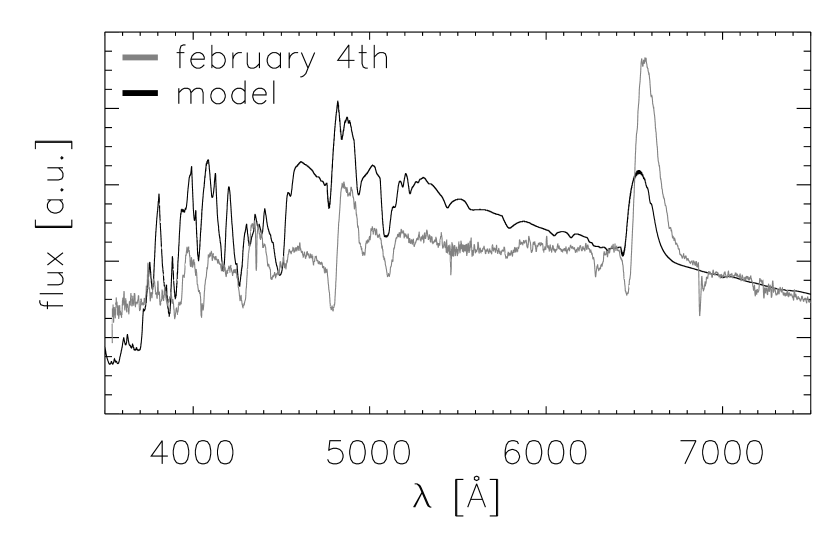
Figure 2: The plot shows the first model that reproduced some of the observed spectral features. No model was found that matched the observed rise of the continuum, hence the extinction inside the parent galaxy appears to be important. The spectra were normalized in such a way that they match the continuum above 6900 Å.

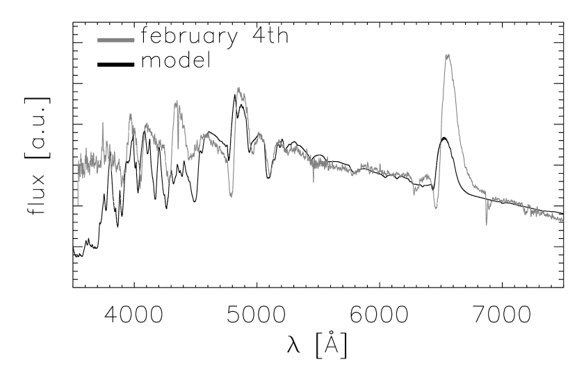
Figure 3: The same model as in Fig. 2 is shown. The observation was dereddened using a higher extinction of $E(B-V)=0.3$. The spectra were normalized to match the continuum above 6900 Å.

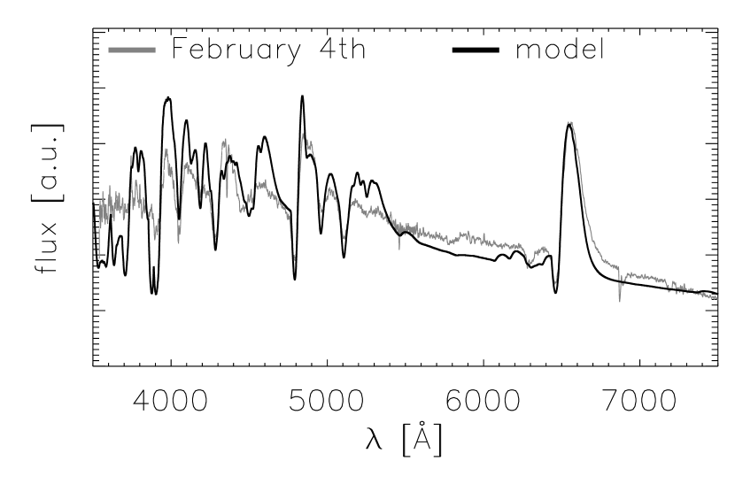
Figure 4: A model is compared to the observation on Feb. 4. Solar abundances are assumed. The other key-parameters are $T_{\rm{model}}=5800$ K and $v_{0}=4900$ $\mbox{km}\leavevmode\nobreak\ \mbox{s}^{-1}$. The observation was corrected for $E(B-V)=0.4$. The spectra were normalized by area.

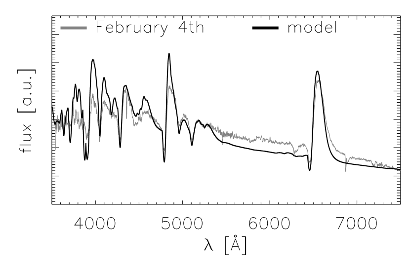
Figure 5: The best fitting synthetic spectrum is compared to the observation on Feb. 4. All model parameters are the same as in Fig. 4 with the exception of the metalicity which is [M/H]$\approx-0.5$. The observation was corrected for $E(B-V)=0.4$. In comparison with the model from Fig. 4 the fit is now much better. The spectra were normalized by area.

The variation of the velocity field was required in order for the models to match the observations. Gradually changing the velocity field resulted in a different wavelength shift and only slightly changing spectral features. No particular velocity could be favoured other another in a range of a few hundred $\mbox{km}\leavevmode\nobreak\ \mbox{s}^{-1}$.

The variation of the velocity was problematic in the first models due to the fact that slower models didn’t converge properly or didn’t reproduce the spectra as well as before. However, due to the refining of the atmosphere structure via inclusion of more NLTE species the models became more robust to the change of the velocity parameter.

In Figs.  5–8 we show the final model spectra for all four observed epochs. In all Figs. the observations were corrected for an extinction of $E(B-V)=0.4$. This change of the extinction from the initial guess is mainly due to the use of non-solar abundances. The under-abundance of the metals increased the flux in the blue part of the spectrum and therefore the observations demanded more de-reddening. In order to support the large reddening that we find, we have searched for Na ID interstellar absorption lines in the host galaxy. Since there is a strong broad SN feature just as the wavelength of the Na ID lines they don’t clearly stand out, but there is a hint of an extra narrow absorption line at the right wavelength. Thus, our somewhat high extinction value is reasonable.

The important model parameters of the different observations are summarized in Table 2.

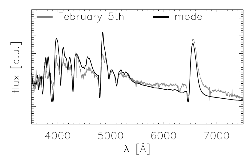
Figure 6: The best fitting synthetic spectrum for Feb. 5 is compared to the observation. The model has $T_{\rm{model}}=5700$ and $v_{0}=4850\mbox{km}\leavevmode\nobreak\ \mbox{s}^{-1}$. The spectra were normalized by area.

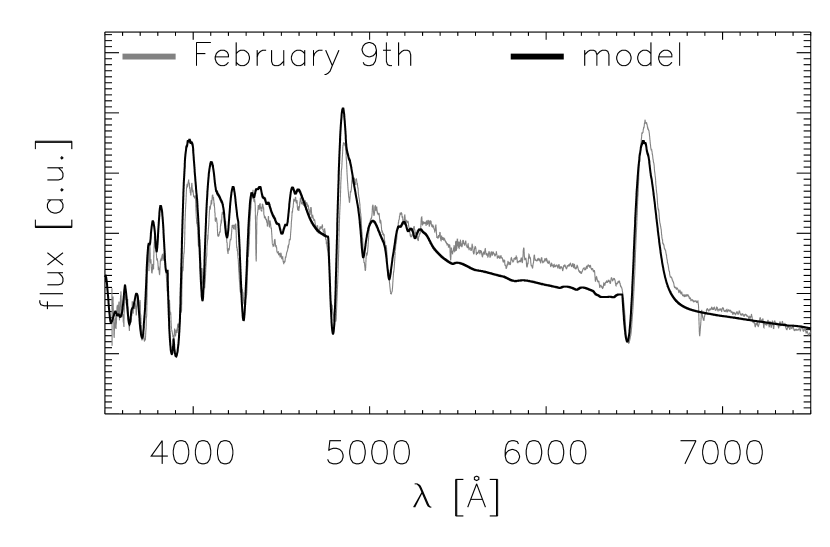
Figure 7: The best fitting synthetic spectrum for Feb. 9 is compared to the observation. The model has $T_{\rm{model}}=5600$ and $v_{0}=4500\mbox{km}\leavevmode\nobreak\ \mbox{s}^{-1}$. The spectra were normalized by area.

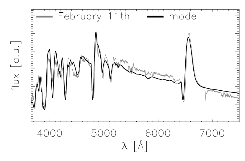
Figure 8: The best fitting synthetic spectrum for Feb. 11 is compared to the observation. The model has $T_{\rm{model}}=5400$ and $v_{0}=4300\mbox{km}\leavevmode\nobreak\ \mbox{s}^{-1}$. The spectra were normalized by area.

5 Conclusion

We have modeled the early spectra of the Type II supernova SN 2003Z. The results show that there is substantial extragalactic reddening towards the SN, probably due to dust in the plane of its parent galaxy. For each observed epoch we have determined the best-fit parameters of the NLTE models as summarized in Table 2.

The best fits require sub-solar metalicities of about [M/H]$\approx-0.5$, indicating that the progenitor of SN 2003Z was a quite metal-poor star (see also Baron et al. (2003)). Unfortunately there are only very few observations available for this object and in particular, no accurate light curve is known, therefore we have assumed that the relative fluxes are accurate. Without photometry we can not calibrate the relative fluxes and thus our results are sensitive to the accuracy of the relative flux calibration.

Table 2: Summary of the basic parameters $T_{\rm{model}}$ and velocity for the different days. There is no error estimation for the velocity as a range of velocities fit the spectra and the given value was just picked to match the observed redshift. The models fit best with metalicities [M/H]$\approx-0.5$, however, there is quite a range of possible values that cannot be ruled completely out, so [M/H]$=-0.5+/-0.3/0.5$. The luminosities are relatively well determined – $\Delta T_{\rm{model}}=\pm 100\mathrm{K}$ – for the assumed extinction, but depend strongly on this parameter. The pressure $p_{0}$ is determined at $\tau=1$ in the radial $\tau$-grid.

February	$T_{\mathrm{model}}$	[M/H]	$v_{0}$	n	$p_{0}$
	[K]		[$\mbox{km}\leavevmode\nobreak\ \mbox{s}^{-1}$]		$[10^{-8}\,\mathrm{bar}]$
4th	5800	-0.5	4900	9	4.43
5th	5700	-0.5	4850	9	5.41
9th	5600	-0.5	4500	9	6.83
11th	5400	-0.5	4300	9	9.76