Abstraction and Refinement in Static Model-Checking

Abstract

Abstract interpretation is a general methodology for building static analyses of programs. It was introduced by P. and R. Cousot in [3]. We present, in this paper, an application of a generic abstract interpretation to domain of model-checking. Dynamic checking are usually easier to use, because the concept are established and wide well know. But they are usually limited to systems whose states space is finite. In an other part, certain faults cannot be detected dynamically, even by keeping track of the history of the states space.Indeed, the classical problem of finding the right test cases is far from trivial and limit the abilities of dynamic checkers further. Static checking have the advantage that they work on a more abstract level than dynamic checker and can verify system properties for all inputs. Problem, it is hard to guarantee that a violation of a modeled property corresponds to a fault in the concrete system. We propose an approach, in which we generate counter-examples dynamically using the abstract interpretation techniques.

Keywords

static analysis, model-checking, abstract interpetation, refinement

I Introduction

Being given that the number of state of a model believes in an exponential way with the number of variables and components of the system, the model-checking became complicated to treat in an automatic way. In order to make this work realizable, it is necessary to reduce the sizes of these models with an aim of reaching time and reasonable memory capacities. The techniques of reduction seek to suppress the harmful effects of the combative explosion. When the graphs of behavior comprise several million or milliards of states and transitions, the physical limits of the memory are quickly reached. It is then necessary to resort to techniques compressions of the graphs of behavior. Most known is based on the BDD (Binary Decision Diagrams). At the enumeration time, to decide if a reached state was already met requires to traverse the explored part of the graph. This subgraph, which does not cease growing bigger, must be arranged in the read-write memory. The limits of this memory are quickly exceeded and the implementation of algorithms of pagination know a considerable fall of performances. The methods of abstraction make it possible to eliminate the proliferation from different states(ones from the other) by possibly unimportant details within sight of the properties to be checked. It is essential that the small-scale model preserve sufficient information to produce the same results as the models of origin and to preserve the same properties that one wishes to check. These two exigences must be considered with attention at the time of the generation of a abstract model starting from a concrete model. To conceive a “good” method of reduction consists to produce a reduction relation verifying three criteria: an important reduction ratio, a relation of strong preservation and an easy deduction of the relation of reduction starting from the description of the system, the ideal being the construction of the reduced graph directly starting from the description. The way whose details of the abstraction will be selected for the checking can be made in an automatic or manual way. The manual technique includes abstract interpretations selected by the user. The abstractions considered generally preserve the properties in a weak way, which means that they are only preserved abstracted model with the concrete model. Thus, if one can guarantee that a property is checked, that is different with its negation. The abstract interpretation is a methodology aiming at defining, analyzes and justifier your techniques of approximate computation of properties of systems in [3]. Whatever the semantics may be used. It then consists in placing the analysis not in the concrete domain but in a abstract domain, (simplified and limited) which conserves the search properties, the major disadvantage is that the results are in general less precise and that one needs accommodate approximations of the properties. In our paper, we present a technique of abstraction called abstraction by predicate of a refinement to reduce the generality and the minimality of the analysis, thus a violation of a property detected on one of abstract path has a strong probability of existing on a path of the concrete model. Analysis is made at the global state space level: traversal algorithm (similar to the one used to build the state space) is used to check out deadlock, livelock or divergent states. Example pathes starting from the initial state and leading to a deadlock, livelock or divergent state can be extracted. To this end, we have to collect during the search of these special states the intermediate state sets reached before them. verication is based on bisimulation minimizations and comparisons .

II Generality

Small Example: The rule of Signs        

       

       

Such that the following diagram commutates

       

       

Consistency (soundness):

$$\forall x,y\in Int:X\times y\in\gamma(\alpha(x)\stackrel{{\scriptstyle\sim}}{{\times}}\alpha(y))$$

II-A Definition

Abstract Interpretation is a general methodologies for automatic analysis of the run-time properties of system.. The problem is that the exact analysis may be very expensive, sometimes through decidable properties may be NP-complete. The idea is to find a decidable approximation which is soundness and calculable.

II-B Mathematical theory of Abstract Interpretation

Often, AI refers to the concept of connection galoisienne a 4-tuple $(C,A,\alpha,\gamma)$ where $C$ and $A$ are complete lattices , $\gamma:A\rightarrow C$ and $\alpha:C\rightarrow A$ are monotonous functions
such as:

$$\begin{array}[]{lll}\forall\beta\in a:&\alpha(\gamma(\beta))&=\beta,\\ \forall C\in C:&\gamma(\alpha(c))&\geq C.\\ \end{array}$$

         
Impossible into practice of generating and analyzing all possible traces of execution for a given program .

II-C Motivation

Abstract interpretation is based on three fundamental ideas :
abstract domain, abstract operators and point fixes computation Abstract domain and abstract operators are used to carry out a program on abstract values. Computation of the fixed point: directs the process on abstract values (define in a certain way the semantics of the program) Objective: To obtain information on the execution and the results of program. Provided that the abstract domain and operators satisfy certain constraints.

II-D Semantics

Its definition has two view points:

• Theoretical associates a meaning to objects handled by the programs.

• Piratical associates a program a semantic function ( stomata).

  $$<{\mathcal{P},e>\stackrel{{\scriptstyle\tau}}{{\longrightarrow}}<\mathcal{P^{\prime}},e^{\prime}>}$$

  $$\mathcal{P}=\tau.\mathcal{P^{\prime}}\mbox{ and }e^{\prime}=\tau(e)$$

  $\tau$ is a transition related. Note:

  $$\tau[\mathcal{P}](e_{0})=cal$$

  if $cal=<\_,e_{n}>$ then the results of the program are the values of variables in the last state.

• Denotational

  $$\tau:(D\longrightarrow D)\longrightarrow(D\longrightarrow D)$$

  $$\tau=\lambda f.\lambda x.(\mbox{ if }p(x)\mbox{ then }x\mbox{ else }f(h(x))\mbox{ fi}$$

  where $p$ is a predicate , h any function. Example F91McCarthy:

  $$\tau=\lambda f.\lambda x.(\mbox{ if }x>100\mbox{ then }x-10\mbox{ else }f(f(x+11)\mbox{ fi}$$

II-D1 Abstract Domain

: Any program $P$ handles data which belong to a $D_{s}$ domain says standard. To make abstract interpretation will consist in choosing an abstraction of data $D_{abs}$ First Approach

$$\theta=\{x_{1}\leftarrow t_{1},\ldots,x_{n}\leftarrow t_{n}\}$$

$\beta$ approximates $\theta$ iff

$$\beta=\{x_{1}\leftarrow prop(t_{1}),\ldots,x_{n}\leftarrow prop(t_{n})\}$$

this define concretes semantics
More often no-calculable.
Construction process $P$ can be consider like a partial function of

$$P:D_{s}^{m}\longrightarrow D_{s}^{n},n,m0$$

Example: function of McCarty known as function91

$$F91(x)=\mbox{ if }x>100\mbox{ then }x-10\mbox{ else }F91(F91(x+11))$$

int F91(int x)
         int F;
                  if (x >100) f =x-10;
                  else f=F95(F95(x+11));          return F;

int F91McCarthy(void){
   int x;
   scanf(&x);
   printf("value of F91 of %d = %d ",
           x, F95(x));
   exit(0);
}

Note:: There is not a proof of termination of $F91McCarthy$, $\forall X\in\mathcal{Z}$
The idea is to replace $Z$ by its power set $\cal{P}(Z)$.
We get the following definition:

$\begin{array}[]{l}F91(X)=\{x-10:x>100\wedge x\in X\subseteq Z\}\cup\\ \mbox{~{}~{}}F91(F91(\{x+11:x\leq 100\wedge x\in X\subseteq Z\}))\\ \end{array}$

It is easy to show that $F91(C_{1})=C_{2}$ verifies the condition: $\forall x\in C_{1}\exists y\in C_{2}:y=f(x)$

Note:: the calculation of such function is too expensive for simple value, the definition of the operations on a such domain is too complex.

Second Approach
To choose ”a good” system of representation of properties

$$\beta=\{x_{1}\leftarrow\alpha(prop(t_{1})),\ldots,x_{n}\leftarrow\alpha(prop(t_{n}))\}$$

Choice of an (judicious) approximation of each element of $\cal{P}(Z)$ by an interval $[min..max]$

$$D_{abs}=\{[s..t]:s,t\in Z\cup\{-\infty,+\infty\}\}$$

we define an order on $D_{abs}$, noted $\subseteq$ : $[s..t]\subseteq[s^{\prime}.t^{\prime}]$ iff $s\geq s^{\prime}$ $t\leq t^{\prime}$

Lemma:

$(D_{abs},\subseteq)$, is a lattice whose lower bound is $[]$ and the upper bound is $[-\infty,+\infty]$. Abstraction and concretization function:

$$\alpha:C\longrightarrow A:C\rightarrow\alpha(c)=[min(c)..max(c)]$$

$$\gamma:A\longrightarrow C:a\rightarrow\gamma(a)=[s,s+1...,t-1,t]$$

with $a=[s..t]$ such that they verifying the constraints of coherence:

$$\forall c\in C:\gamma(\alpha(c))\supseteq c\\ \forall a\in A:\alpha(\gamma(a))=a.$$

Remark

• an equivalent abstract of a program carries out the same standard operations that the original except that the domains are different.

• for a real Pascal, C or Java programs, the work of rewrite would be too tiresome. In fact one defines abstracted operators, the abstract interpretor uses those to carry out calculations on the abstract data by interpreting the program to be analyzed.

• In practice each operator or function of the language must have an abstract equivalent. The quality required is their consistency, their coherency with respect to their equivalent concrete operator. For the reason of performance, one requires the efficiency and convergence to guarantee a termination and acceptable computing time.

Abstract version of the F91 function:

$\begin{array}[]{ll}F_{a}91([s..t])=&[max(91,s-10)..(t-10)]\cup\\ &F_{a}91(F_{a}91([(s+11)..min(t+11,111)]))\end{array}$

$\begin{array}[]{ll}\forall I_{i},I_{j}\in D_{a}:&I_{i}=[s..t],I_{j}=[s^{\prime}..t^{\prime}]\Rightarrow\\ &I_{i}\cup I_{j}=lub(I_{i},I_{j})=[min(s)..max(t,you)],\end{array}$ The abstract calculus:

$$F_{a}91([-\infty..+\infty])=[91,+\infty]\cup\\ F_{a}91(F_{a}91([-\infty..,111]))$$

$$F_{a}91([-\infty..111])=[91,101]\cup\\ F_{a}91(F_{a}91([-\infty..,111]))$$

Note:: The set of functions of $D_{a}\longrightarrow D_{a}$ can be provided with an order $f\leq G$ iff $\forall I\in D_{a}:f(I)\subseteq g(I)$
The fixpoints calculus: it is useful at the time of the recursive calls, to ensure the termination while proceeding by successive approximations.

Complete lattice

• a lattice iff $\exists\bot\in D$ and $\exists\top\in D$

• complete iff

  • $\forall X\subseteq D\exists U\in D:\forall X\in Xx\leq U$ and

  • $\forall X\subseteq D\exists L\in D:\forall X\in Xx\geq L$

It is obvious thats $(D,\leq)$ satisfy this conditions.

Monotonicity and continuity

Let $A$ be a complete lattice with a partial order $\leq$ and $T:A\longrightarrow A$ a transformation

• $T$ is monotonous iff $\forall X,y\in a:X\leq y\Rightarrow T(x)\leq T(y)$

• $T$ is continuous iff $\forall X\subseteq a:T(lub(X))=lub(T(X))$

The transformation that we consider is a functional from a set of function in i ts self.

$$T:(D_{a}\longrightarrow D_{a})\longrightarrow(D_{a}\longrightarrow D_{a})$$

$\begin{array}[]{l}(TF_{a}91)([s..t])=[max(91,s-10)..(t-10)]\cup\\ F_{a}91(F_{a}91([(s+11)..min(t+11,111)]))\end{array}$

Lemma:

T is continuous and monotonous:

• $\forall I_{i},I_{j}\in D_{a}:I_{i}\leq I_{j}\Rightarrow f(I_{i})\leq f(I_{j})$

• $\forall I_{1}\subseteq I_{2}\subseteq...\subseteq I_{n}\subseteq...\Rightarrow f(\cup_{i=1...\infty}I_{i})=\cup_{i=1...\infty}f(I_{i})$

Theorem Let $f([s..t])$, the computing fixpoint consist of $T$ to $f([s..t])$.

• If the constraints on the domain and the operators are satisfied:
  then any fixpoint of $T$ is a correct approximation of the function $f$

• the smallest fixpoint of $T$ exists and constitutes the best approximation of $f$

• the smallest fixpoint of $T$ coincide with the limit of an increasing

• the smallest fixpoint of $T$ coincide with the limit of an increasing sequence of approximation: $f_{0}\leq f_{1}\leq f_{2}\leq f_{0}...\leq f_{n}\leq...$
  such as:   $f_{0}(I)=\bot~{}\forall I\in D_{a}$
  $f_{k+1}=T(f_{k}>)~{}\forall k\geq 0$

II-D2 Fixpoint Approach

Fixpoint Approach is based on the monotonicity (continuity) of the transformation of the tuples set representing the pre and post condition for all predicate. Termination of the algorithm in the case of an infinite abstract domain, it did not guarantee. Which is the case if one makes an infinity different recursive call. One can limit oneself to abstract fields finished in certain cases that can averrer genant itself or unacceptable. A possible solution, would be to replace an infinite sequence of approximation by a number of the approximate values.

Approach Widening/Narrowing

Suppose the abstract semantics of the program given by a function $f_{P}:D_{abs}\longrightarrow D_{abs}$. The analysis proceeds as follows:

1. Widening: calculation of sequences limit $X$ built by:

   • $x_{0}=\bot$

   • $x_{i+1}=x_{i}\mbox{ and }f_{P}(x_{i}))\sqsubseteq x_{i}$

   •           else$x_{i}\bigtriangledown f_{P}(x_{i})$

   • Narrowing to improve the result obtained by the widening: by

   calculating the sequences limit of $Y$ built by:

   • $y_{0}=\sqcup X$

   • $y_{i+1}=\mbox{and}f_{P}(y_{i})=y_{i}\mbox{then}y_{i}$

   •            else $y_{i}\bigtriangleup f_{P}(y_{i}))$

Properties

1. Widening: $\bigtriangledown:l\times L\longrightarrow L$   $\forall X,Y\in L:~{}~{}X\sqsubseteq Y\bigtriangledown Y$ and $Y\sqsubseteq X\bigtriangledown Y$
   $\rightarrow X\sqcup Y\subseteq X\bigtriangledown Y$
   $\bot\bigtriangledown X=X\bigtriangledown\bot=X$

2. Narrowing $\bigtriangleup:l\times L\longrightarrow L$
   $\forall X,Y\in L:~{}~{}Y\sqsubseteq X\Rightarrow Y\subseteq X\bigtriangleup Y\sqsubseteq X$
   

Widening applied to the intervals

$$\begin{array}[]{ll}[l_{0},u_{0}]\bigtriangledown[l_{1},u_{1}]=&[\mbox{ and }l_{1}u_{0}\mbox{then}+\infty\mbox{else}u_{0}]\\ \end{array}$$

Example instead of making the recursive call with $F_{a}91([-\infty..111])$ one will do it with $F_{a}91([-\infty..+\infty])$. But a loss of precision would be introduced. This will allow to speed up the computation of the fixpoint.

III Refinement

Motivation

The abstract interpretation framework establishes a methodology based on rigorous semantics for constructing abstraction that overapproximate the behavior of the program, so that every behavior in the program is covered by a corresponding abstract execution. Thus, the abstract behavior can be exhautively checked for an invatiant in temporal logic. Refinement guided by counterexample consist on approximation of the set of sates that lie on a path from initial state to a bad state which is successsively refine that is done by forward or backward passes. This process is repeated until the fixpoint is reached. If the the resulting set of state is empty then the property is proven. Otherwise, yhe methode does not guaranties that the contreexample trace is genuine.

III-A Preliminaries

Definition III.1

Theorem III.1

Cousot77
Let $S=(Q,Q_{init},\sum,\rightarrow)$ a system representing the semantics of program. The system $S^{A}=(Q^{A},Q_{init}^{A},\sum,\rightarrow^{A})$ is an abstraction of $S$ $\iff$ there exists a Galois connexion:
$\alpha:\mathcal{P}(Q)\longmapsto\mathcal{P}(Q^{A}),\gamma:\mathcal{P}(Q^{A})\longmapsto\mathcal{P}(Q)$
such that

• $Q_{init}\subseteq\gamma(Q_{init}^{A})$

• $\forall\tau\in\sum,\forall Q_{i}^{A}\subseteq Q^{A}.post[\stackrel{{\scriptstyle\tau}}{{\rightarrow}}](\gamma(Q_{i}^{A}))\subseteq\gamma(post[\stackrel{{\scriptstyle\tau^{A}}}{{\rightarrow}}](\gamma(Q_{i}^{A}))$

Definition III.2

Predicat Abstraction Graf&Saidi97

Abstract State

Let $Prog=(\mathcal{V,T}=\{\tau_{1},\ldots,\tau_{n}\},Init)$ and $\varphi_{1},\ldots,\varphi_{k}$ predicates over the $Prog$’s variables
we define an abstraction $S^{A}=(Q^{A},Q_{init}^{A},\sum,\rightarrow^{A})$ as following:

• $Q^{A}=B^{k}$ , $Q^{A}$ is the valuations’ set of $k$ boolean variables,
  any subset $Q^{A}$ can be represented by a boolean expression over the variables $B_{1},\ldots,B_{k}$

• $S^{A}$ as the form $Prog^{A}=(\mathcal{V}^{A},\mathcal{T}^{A}=\{\tau_{1}^{A},\ldots,\tau_{n}^{A}\},Init^{A})$

Abstract transition

Let $\mathcal{T}^{A}$, be an abstract transition, it must satisfy the condition of the definition of abstract program , s.t. all transition $\tau$, $post[\tau^{A}](P_{B})$, where $\tau^{A}$ is the abstract transition corresponding to $\tau$, have to represent all concrete states $q^{\prime}$ which are successors by $\tau$ of concrete state $q$ represented by $P_{B}$. We must show :: $post[\tau](\gamma(P_{B}))\Rightarrow\gamma(P_{B}^{{}^{\prime}})$,

III-B Algorithmic checking of refining

This model-checking needs methodological and correctness conditions:

III-B1 Methodological conditions

• New actions and variables will be introduced by refining

• the variables of refine system and abstract system must be linked by a “collage” invariant.

III-B2 Correctness conditions:

• simulation of the refine system by the abstract

• no cycle between the new action

• no new deadlock

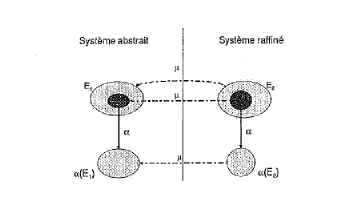
Figure 1: Simulation with old actions

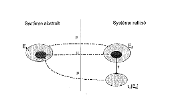
Figure 2: Simulation with new actions

It is a question of carrying out an iteratif calculation of the simulation of $TS_{2}$ by $TS_{1}$ cfr figures 1 and 2 where transisition $\alpha$ is replace by $\tau$. The algorithm terminates when the fixpoint is reached.

Theorem III.2

• If $P_{1}$ is property satisfied by $TS_{1}$ and $TS_{2}$ refines $TS_{1}$ then

  $$\frac{TS_{1}\models P_{1},\vdash TS_{2}\subseteq TS_{1}}{TS_{2}\models P_{1}}$$

• If $P_{1}$ is property satisfied by $TS_{1}$ and $TS_{2}$ refines $TS_{1}$ and if $P_{2}$ is a reformulation of $P_{1}$ then

  $$\frac{TS_{1}\models P_{1},\vdash TS_{2}\subseteq TS_{1}}{TS_{2}\models P_{2}}$$

Definition III.3

: Let K, K’ two systems (resp concrete and abstract). we call false-counterexample or negative-false a false universal property in K’ but true in K We say that the counterexample specified in K’ cannot be reproduced in K

Corollary

If K’ is too small, it is very probable that it appears the negative one. If K’ is too large, then the checking is not possible the refinement guided by counterexample is thus a natural approach to solve this problem by using a adaptive algorithm which gradually creates an abstraction function by the analysis of false-negative:

Pseudo Algorithm

1.	Initialization:
	generate a first abstraction function;
2. Model-Checking:
	check the model.
	if	the checking is a success:
		then
			the specification is correct and
			the algorithm terminates
		else
			generate a counterexample from the abstract model
			verify if this counterexample is a negative-false
			if It is a success then terminate
			else refine the abstract function such that
			the negative-false can be avoid
			goto step 2.

Figure 3: Example of predicate abstraction

Figure 4: abstraction too coarse

Figure 5: Example of refinement

IV Summary

It is thus a question of starting by carrying out an approximation of a way which carries out initial state in a bad condition. Then, a refinement ”forwards” or ”backward” is carried out, and this process is to repeat until a fixpoint is met. If the resulting set of states is empty then the property is prove, since one no bad condition is reachable, else, nothing guaranteed the value of against example which perhaps distorted by approximation coarse. Heuristics is employed to determine the subset of the reachable states since the initial states. If an equivalence is found, it really acts of an error which can be deferred like a bug, one speaks about positive-false. Abstraction by Predicate : the checking of program by abstraction of closed predicate is a technique of checking of program by abstract interpretation where the abstract domain is composed of the set of guard relating to the states and the transitions from the system. This domain can be generated automatically and checked by a theorems-prover. Like, the set of predicates is always finished, it can be coded by a vector of Boolean, which makes it possible on the other hand to use the model-checker for calculations of fixpoint.Si, the domain is very large, one can use a chaotic iterator and to use a widening if it is necessary of speed up the convergence. The termination and reachability decidable in this case. The one limitation of this technique of checking by predicate abstraction is that the processes of refinement, which primarily consists in calculating the weakest invariant, are extremely slow. This obligates the users to require at least the atomic predicate necessary to the proof. This fact the human intervention which specific is given must be repeated for different programs even if they are very similarities. and it

V Conclusion and Future Work

It has been shown that static checker can cover a large number of potential faults, their automatic usage is still far from realistic. However, as a verification step prior to testing or code review, static checkers, can already enhance the software development process today. Several techniques like Altarica, B or CSP2B were proposed to specify and check reactive systems by using hierarchic development by refinement. In this case, the systems design is realized gradually by increasing the systems design to each step of the specification from a very abstract sight of the system until its implementation. For us, a system implements (refines) another system if all the traces of execution of the most detailed system are too traces of the most abstract ( modulo the introduction of details during refinement). The checking of the system thus will use refinement to model the initial system in a more precise way, if the model-checker provides a erroneous result consequence of coarse approximation at the time of the abstraction.

References

- [1] André Arnold, Gérald Point, Alain Griffault Antoine Rauzy: The AltarRica Formalisme for describing concurrent systems. Nov. 1999, Fundamental Informatica Volume 40 issue 2-3, Publisher: IOS Press,
- [2] Edmound Clarke Contreexemple-guided abstraction refinement. In 10Th International Symposium on Temporal Representation and Reasonning and Fourt International Confernce on Temporal Logic, 2003.
- [3] P. Cousot, R. Cousot Abstract Interpretation: A Unified Lattice Model for Static Analysis of Programs by Construction of Approximation of Fixpoints, POPL 1977, Sigact Sigplan, pp 238–252.
- [4] T. Kanamori, T. Kawamura Analysing success patterns of Logic Programs by Abstract Hybrid Interpretation, Technical report, ICOT, 1987.
- [5] B. Le Charlier, K. Musumbu, P. Van Hentenryck A generic abstract Interpretation algorithm and its complexity analysis, In Proc ICLP 91, June 91.
- [6] D. Knuth Semantics of context-free languages; Math. Systems Theory 2 (1968), pp 127-145, 5th ICLP–SLP 88;tutorial No2.
- [7] T. Henzinger, R.Jhala, R.Majumdar, G. Sutre Lazy abstraction ; Technical report University of California and LaBRI, 2002.
- [8] David Déharde Interpr tation abstraite: introduction et applications l’analyse statique et la v rification de mod les; Technical report LORIA, 2002
- [9] T. Ball, A. Podelski, S. Rajammani Boolean and cartesian abstractionfor model checking C programs. ; Technical report LORIA,Microsoft Corporation, 2000.