A Simple Way to Distribute Mathematica Evaluations

Abstract

We present a simple package for distributing evaluations of a Mathematica function for many arguments on a cluster of computers. After setting up the hosts, the only change is to replace Map[f, points] by MapCore[f, points].

1 Introduction

With the fairly recent arrival of low-cost multi-core CPUs, institutes often have significant computing power at their disposal. Mathematica 7, whose main motto is parallel computing, makes it relatively simple to send a calculation to the fellow cores on the same machine, though still not exactly straightforward to distribute a calculation on a larger cluster. The package we present in the following fills this gap. After a one-time setup of the cluster, it allows to easily distribute calculations to as many hosts as there are Mathematica licenses available (both ordinary licenses and Mathematica 7’s sublicenses).

We certainly do not propose to parallelize ‘atomic’ Mathematica operations, like Simplify, which is a daunting task even at the conceptual level. Rather, we focus on lengthy evaluations of one function over many arguments, for example the evaluation of a cross-section for many points in phase and/or parameter space. Incidentally, our package is not restricted to numerical evaluations, but can handle any kind of Mathematica expressions.

Many physicists would argue that at least numerical evaluations of a certain volume should be done in a compiled language for performance reasons. This is at best partially true, as Mathematica has a formidable arsenal of functions, e.g. for numerical analysis, which are not easily available elsewhere, and it is the choice of algorithm that influences the computation time much more than the speed of a single evaluation. Furthermore, in conjunction with MathLink, e.g. through FormCalc’s Mathematica interface [2], the execution speed is essentially that of a compiled language and Mathematica’s part is ‘governing’ the calculation.

The package we present in this paper is remarkably short and contains one main function MapCore which substitutes Map in serial calculations. Sect. 2.1 describes usage of the package, Sect. 3 provides a function reference, and Sect. 5 describes installation and system setup.

2 Overview

2.1 Usage of the MultiCore package

The MultiCore package is loaded with

   << MultiCore‘

The next step is to add cores on which evaluations can be distributed. This can be done directly with e.g.

   AddCore["pc123.mppmu.mpg.de"]

or, if login under a different username is required,

   AddCore["batman@pc123.mppmu.mpg.de"]

This explicit method becomes cumbersome, however, if many cores with varying loads are involved. The alternate invocation

   AddCore[10]

takes up to ten of the currently ‘free’ cores. This information is supplied by the findcores shell script (part of the MultiCore package) which in turn reads the admissible cores from a .submitrc file and invokes ruptime to determine the load. The .submitrc file has the simple syntax

   pc380   4
   pc381   4
   pc339b  2
   pc472

where the optional integer behind the hostname indicates the number of cores the host has. The machines should be listed in descending CPU speed, i.e. fastest on top, to optimize performance. Each remote host should be running an rwhod daemon, since then its load will be reported through ruptime and findcores will use only the free cores.

In the case of a Linux cluster, the .submitrc file can be generated (more or less) automatically, with the help of the setupcores script, as in:

   ./setupcores > $HOME/.submitrc

This script assumes that the hosts are listed via ruptime, that a password-free login via ssh is possible, and that each host is running a flavour of Linux where /proc/cpuinfo can meaningfully be read out. The file generated in this way constitutes a ‘raw’ version and should be reviewed by hand.

Each core launched requires a Mathematica license, i.e. a Kernel license. From Mathematica 7 on, each (main) license includes four sublicenses and it is possible to use these sublicenses for parallelization (cf. Sect. 3.11, $SublicenseFactor).

One can further take care not to invoke more slave processes than licenses available. To this end AddCore is invoked with an integer $n\leqslant 0$, meaning that it should spawn at most so many slaves that $|n|$ (main) licenses are left for other users. Also one can provide a second integer argument $m\leqslant 0$ to leave $|m|$ sublicenses unused. This mode really makes sense only for network licenses. For non-network licenses, AddCore silently assumes that the other machines listed in .submitrc have similar licenses.

MultiCore generally works in a master–slave model, requiring one license (but hardly any CPU time) for the master and one main or sublicense for each slave. We assume that all cores in the cluster run the same Mathematica version, in particular that the master’s version number is the same as all slaves’. In particular we assume that subkernels on slave cores can be launched if and only if the master is running Mathematica 7.

Quitting the master’s Mathematica Kernel automatically closes all links, so explicitly ‘removing’ registered cores is usually not necessary unless one wants to free Mathematica licenses. Each slave session is characterized by an identifier of the form host[id], where host is the host name and id an integer link id. The syntax for RemoveCore is

   RemoveCore[host]
   RemoveCore[host[id]]

where both host and id may be a pattern. Thus, RemoveCore["pc123"] closes all slaves on host pc123 and RemoveCore[_] closes all current slave sessions.

Once the cores are registered, the only necessary substitution is to replace Map (/@) by MapCore to make multiple evaluations execute in parallel.

Important: The only slightly non-straightforward aspect is the remote definition of the function being evaluated. MapCore sends the definition of this function to the slave as much as the Save function would save it in a file. This fails to work (for both MapCore and Save) if the function depends on a LinkObject in the master’s session, i.e. if the function is or invokes a MathLink function. Even if the slave session has the same MathLink executable installed, it will in general not communicate via the syntactically same LinkObject.

To work around such cases, the AddCore function has an optional second argument. This argument is sent to the slave upon opening of the link as an initialization command. In our opinion the best procedure in the MathLink case mentioned above is not to install the MathLink executable in the master’s session at all, to prevent sending any explicit LinkObject pointing to the master’s installed MathLink executables, and instead include the Install statement in the AddCore invocation, as in

   AddCore[0, Install["LoopTools"]]

Also, if the function has a very lengthy definition one might want to place it in a file and load that via the initialization command, e.g.

   AddCore[0, << myfunction.m]

Of course one would have to submit this file to each slave first if they do not have access to the master’s filesystem. Note, however, that the slaves’ working directory is the user’s home directory, not the current working directory on the master. In other words, the file to be loaded must include a path unless it resides in the home directory anyway.

2.2 MultiCore’s concurrency handling

MapCore tries to have the given points calculated as quickly as possible. Therefore it distributes more (less) than $\mathit{patchsize}$ points to faster (slower) cores by evaluating its internal timing statistics. Once all points of the list are distributed, MapCore redistributes the unfinished points until the result for all points are available. It automatically decreases the patchsize according to the remaining list size, too. Although due to the competition $N-1$ cores are not yet finished when MapCore returns, the time until all slaves are again ready is negligible. The identifier $CallID helps MapCore to distinguish between new and old data of multiply distributed points.

2.3 MultiCore’s error handling

Especially during long parallized calculations of many CPU-time-expensive points, link error handling plays an important role. If the link to one host, i.e. one or more cores, is lost, MapCore redistributes the as yet uncalculated points to the remaining hosts, executes the equivalent RemoveCore call and prints a warning message. After MapCore has returned one might want to add the lost host by re-invoking AddHost.

3 MultiCore package Function Reference

3.1 AddCore

AddCore adds (registers) cores, i.e. opens links to remote machines for subsequent distributed evaluation with MapCore. It is invoked in one of the following ways:

• AddCore[$\mathit{hostname}$] adds one core on $\mathit{hostname}$ using a main license.

• AddCore[$\mathit{hostname}$, "subkernel"] adds one core on $\mathit{hostname}$ using a sublicense.

• AddCore[$\mathit{n}$] ($\mathit{n}>0$, integer) adds up to $\mathit{n}$ cores using the findcores script (described below) using a ratio $SublicenseFactor : 1 of sublicenses to main licenses (cf. Sect. 3.11).

• AddCore[$\mathit{n}$] ($\mathit{n}\leqslant 0$, integer) adds as many cores as there are main licenses using findcores, but leaves at least $|\mathit{n}|$ main licenses for other users.

• AddCore[$\mathit{n}$, $\mathit{m}$] ($\mathit{n},\mathit{m}$ integer) same as above, with $\mathit{n}$ for main licenses and $\mathit{m}$ for sublicenses.

The last two invocations really make sense only for network licenses. For non-network licenses, it is silently assumed that the information taken from $LicenseProcesses and $MaxLicenseProcesses (in the master’s session) holds also for the remote cores. Each link corresponds to one core on a remote machine. It is hence permissible to add the same host more than once, to account for its number of cores. The links are identified, apart from the hostname, by a unique integer link id. This id is also sent to each slave process as $CoreID and can be used to e.g. construct unique filenames. Core additions are cumulative. Links are released either through explicit removal with RemoveCore or by quitting the master’s Mathematica Kernel.

The findcores script is part of the MultiCore package. It needs a .submitrc file in which the admissible cores for distributed computing are listed. Each line has the syntax

   hostname   [# of cores]

Comment lines starting with a # are allowed. Cores are processed in sequential order, i.e. the fastest machine should appear at the top of this list. The .submitrc file is searched for in the following order:

• ./.submitrc,

• $HOME/.submitrc,

• $\mathit{(MultiCore\,installation\,directory)}$/submitrc,

• /usr/local/share/submitrc.

findcores invokes ruptime to determine the load on a remote machine. This works only if the remote machine is running an rwhod daemon. If not, the load is assumed to be zero, i.e. all cores are taken.

3.2 RemoveCore

RemoveCore removes (unregisters) cores from the internal list, shuts down the corresponding remote kernels and closes the links. Each core is identified by two quantities, the hostname and the link id. Calling RemoveCore is usually not necessary, as quitting the master’s Mathematica Kernel automatically closes all links.

• RemoveCore[$\mathit{hostname}$[$\mathit{id}$]] removes all cores matching $\mathit{hostname}$ and $\mathit{id}$, where either may contain a pattern. For example, RemoveCore[_] removes all links, and RemoveCore["pc456"[_]] removes all links to pc456.

• RemoveCore[$\mathit{hostname}$] is equivalent to RemoveCore[$\mathit{hostname}$[_]].

3.3 ListCore

ListCore lists the currently registered cores.

• ListCore[$\mathit{hostname}$[$\mathit{id}$]] lists all cores matching $\mathit{hostname}$ and $\mathit{id}$, where either may contain a pattern. ListCore[_] thus lists all cores.

• ListCore[$\mathit{hostname}$] is equivalent to ListCore[$\mathit{hostname}$[_]].

3.4 MapCore

MapCore is the main function of the MultiCore package. It substitutes Map in serial calculations.

• MapCore[$\mathit{f}$, $\mathit{points}$, $\mathit{patchsize}$] distributes the computation of $\mathit{f}$ for all items in $\mathit{points}$ to the cores previously registered with AddCore.

The integer argument $\mathit{patchsize}$ is optional (default value: 5) and tells MapCore how many points on average should be sent to each core. As every set of results returned by a slave contains timing information, the master distributes points according to the slaves’ performance. Until the master has gathered enough statistics about the slaves’ timings it sends exactly $\mathit{patchsize}$ points to each core.

The larger the computation time for a single point is, the smaller $\mathit{patchsize}$ should be chosen. A smaller value may also be profitable if the participating cores have significant differences in speed. A $\mathit{patchsize}$ of 1 achieves the best load-levelling but incurs the highest communication overhead. We have generally found the communication overhead to be negligible if the computation time for one patch is several seconds or more (see also performance tests in Section 4).

3.5 RemoteMath

RemoteMath encodes the invocation of a remote Mathematica Kernel. It receives one arguments and one flag, the hostname and the type of license which shall be used while launching the kernel. If required one can define different invocation strings for different hosts.

• RemoteMath[$\mathit{host}$, $\mathit{opt}$] := $\mathit{remotestring}$ defines $\mathit{remotestring}$ as the command for invoking a remote Mathematica Kernel on $\mathit{host}$. Options for the remote kernel are given in $\mathit{opt}$, which is presently restricted to -subkernel for launching a subkernel.

The default command is

ssh (host) ’exec /bin/sh -lc \
  "test ‘uname -s‘ = Darwin && nice -19 MathKernel (opt) -mathlink \
                            || nice -19 math (opt) -mathlink"’

This is an ssh command which starts a remote login shell that executes, with nice 19, MathKernel on MacOS and math on other systems. Starting a login shell is important as it sources the shell’s initialization files, which may modify the PATH.

If the Mathematica Kernel executable cannot be started using this command because it is not on the PATH, we recommend adding the appropriate directories to the PATH on the remote system rather than modifying the RemoteMath definition.

3.6 RemoteMap

With RemoteMap one can specify a mapping function which shall be applied on all remote hosts, i.e. slave sessions, to the point patches they receive from the master. Its default

RemoteMap[f_, points_] := Map[f, points]

is the usual Map function. This may be overwritten with an individual function which must have the same argument structure as Map[$\mathit{f}$, $\mathit{points}$]. This feature could for example be used to leave a part of the parallelization to Mathematica 7 using the ParallelMap function. In that case one of course would set the number of cores in .submitrc to 1 for all hosts.

3.7 $FindCores

$FindCores contains the full path to the findcores script, including (if necessary) any options. The full syntax of findcores is:

   findcores [-f rcfile] [-h ruptimehost]

where rcfile specifies the explicit location of the submitrc file (see Sect. 3.1) and ruptimehost specifies the host on which to invoke ruptime to find out the load of the machines listed in the submitrc file. The latter is necessary if running the master process on a machine not connected to the cluster, e.g. a laptop.

Note: changing $FindCores modifies subsequent invocations of AddCore only, i.e. links once established are not changed by a different value of $FindCores.

3.8 $MsgLevel

$MsgLevel specifies how verbose the master–slave communication is reported on screen.

• $MsgLevel = $\mathit{n}$ sets the message level to $\mathit{n}$.

  The default message level is 1, which just reports the adding and removing of cores as well as link failures.

3.9 $CoreID

$CoreID is unique identifier for each slave session.

• $CoreID (in the master’s session) is the id of the last slave session spawned. This number should not be tampered with.

• $CoreID (in the slave’s session) is a unique identifier of the session.

3.10 $CallID

$CallID is available in both the master and slave session. In the master session it counts the total number of calls to MapCore. In the slave session it identifies that certain call to MapCore which invoked the last computation on this slave. Note that they do not have to be equivalent (see Sect. 2.2).

3.11 $SublicenseFactor

The integer $SublicenseFactor is a global parameter in the master session which is set to 4 if the Mathematica version is 7 or above, and 0 otherwise. Only AddCore[$\mathit{n}$] with $n>0$ makes use of it to decide how many sublicenses should be used launching a kernel before using another (rare) main license. Setting $SublicenseFactor manually only makes sense if one uses Mathematica 7 and wants to optimize it to the mean ratio of unused sublicenses to unused main licenses which might be greater than 4 in some cluster networks.

3.12 $ListPositions

$ListPositions is available in the slave session only. This list contains the positions of the points in the original list which are to be evaluated by the slave.

Both $CallID and $ListPositions can e.g. be used to construct unique filenames. For example, if a single evaluation is very costly in CPU time, one may want to store each result immediately after computation. This could be solved through a wrapper function

RemoteMap[f_, points_] :=
  MapThread[store[f], {points, $ListPositions}]

store[f_, dir_:"results"][x_, i_] :=
Block[ {file = ToFileName[dir, ToString[i]]},
  If[ FileType[file] === File,
    Get[file],
  (* else *)
    If[ FileType[dir] === None, CreateDirectory[dir] ];
    (Put[#, file]; #)& @ f[x] ]
]

Results for each point would be stored in results/$\mathit{n}$, where $\mathit{n}$ is each point’s index in the original list. In addition to $ListPositions one could use $CallID to generate unique filenames over multiple invokations of MapCore in the same master session.

4 Performance Tests

We tested the performance and scalability properties of MultiCore on both a homogeneous and inhomogeneous cluster of 25 cores for different evaluation times per point (tpp) and different patchsizes. As a testing function we used a simple pause directive

  f[p_][x_] := (Pause[p]; x)

and mapped it over 10000 resp. 1000 arbitrary points for different numbers of cores ranging from 0 (local evaluation), 1 (slave) to 25 (slaves) and pausing times $p=0.01,0.1,1$ seconds.

In case of the homogeneous cluster we assumed a constant ‘evaluation’ time per point for each core. In the ideal case one would expect the total time to be inversely proportional to the number of cores. The three inverse plots on the left-hand side of Figure 1 illustrate this ideal connection (blue line) and the deviation of the measured timings for different patchsizes. We took the average of ten independent runs for each point. As one can see, MultiCore’s performance in a homogeneous cluster barely depends on the (reasonable choosen) patchsize. It shows an almost perfect scaling behaviour for evaluation timings per point of around 0.1 seconds or more. For smaller tpp’s one would better choose a bigger patchsize.

To simulate an inhomogeneous cluster we linearly spread the tpp’s from e.g. 1.0 to 4.0 seconds over the range of the 25 cores. On a subset of e.g. 14 cores we of course added the 14 fastest ones. Due to the different evaluation timings the ideal curve is no longer a line. Instead, in the ideal case the total time $T$ depends on the number and performance of the added cores:

$$\frac{1}{T}=\frac{1}{n}\sum_{i=1}^{N}\frac{1}{\text{tpp}_{i}}$$

with $\text{tpp}_{i}$ being the tpp of core $i$ and $N$ the number of cores and $n$ the total number of points. The three plots on the right hand side of Figure 1 show the testing results for different tpp’s (of the fastest core) and for different patchsizes. Again, the patchsize is not a crucial parameter. As before, deviations occur for the small tpp = 0.01 sec. The scaling behaviour for large numbers of cores seems to be at most satisfactory since MultiCore’s parallalizing takes about twice as long as the ideal case predicts. But if one compares the total timings of 25 unequal cores to the corresponding timings on the left hand side, one sees that it takes only about 10 cores from the homogeneous cluster to do the same job. Therefore one principally has to consider the performance gain before joining much slower cores to one’s cluster.

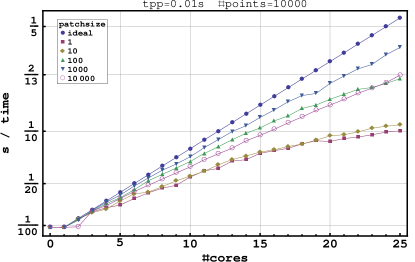
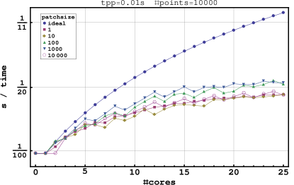
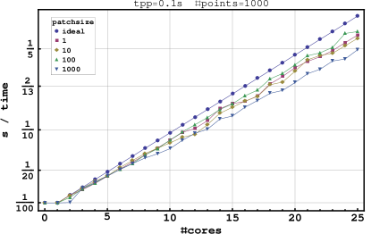
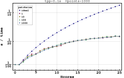
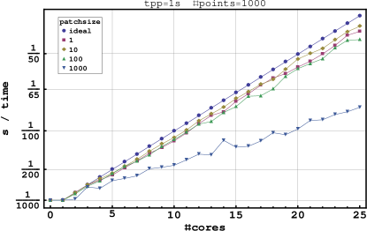
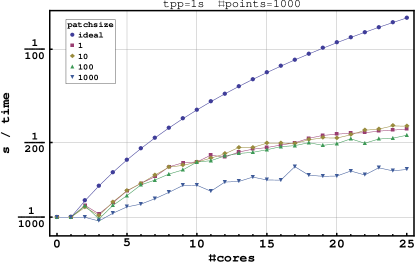
Figure 1: Reciprocal total timings as a function of number of cores for different evaluation times per point (tpp), different number of points (see heading of corresponding plot) and patchsizes. The left column shows the result for the homogeneous cluster ($\text{tpp}_{i}=\text{tpp}_{1}=\text{const}$). The right column shows those for the inhomogeneous cluster i.e. $\text{tpp}_{i}=\text{tpp}_{1}(1+3\,\frac{i-1}{24})$ for $i=1,\ldots,25$.

5 Installation and System Setup

The MultiCore package is available from http://www.feynarts.de/multicore. Installation is as simple as unpacking the tar file. MultiCore requires Mathematica versions 5 and up (version 7 preferred).

To be able to load MultiCore regardless of the current directory, the MultiCore installation directory has to be added to Mathematica’s $Path, for example by placing a statement like

   PrependTo[$Path, "/my/path/to/MultiCore"]

in $\mathit{prefdir}$/Kernel/init.m, where $\mathit{prefdir}$ is one of

• /usr/share/Mathematica (system-wide, Linux),

• $HOME/.Mathematica (user-specific, Linux),

• /Library/Mathematica (system-wide, MacOS),

• $HOME/Library/Mathematica (user-specific, MacOS),

• $ALLUSERSPROFILE/Application Data/Mathematica (system-wide, Cygwin),

• $USERPROFILE/Application Data/Mathematica (user-specific, Cygwin).

The package has been tested under Linux, MacOS, and Windows/Cygwin, both as master and as slave. The communication with remote Mathematica Kernels requires attention to a few details that may not be obvious:

• An sshd daemon must be running on the remote machine and access not restricted by a firewall. On Cygwin one has to start sshd once with “net start sshd” (as Administrator) and on MacOS one has to open the ssh port in the firewall (System Preferences – Sharing – Remote Login).

• ssh access to remote machines must be possible without password authentication. This requires that a host key is generated with ssh-keygen and the public part of it (typically $HOME/.ssh/id_rsa.pub) copied to $HOME/.ssh/authorized_keys.

• If remote access other than by ssh is required, one needs to redefine the RemoteMath function, which encodes the command string used to execute remote Mathematica Kernels (see Sect. 3.5). This can either be done in the master session before any AddCore invocations, or once and forever in MultiCore.m.

6 Summary

The MultiCore package provides a simple mechanism to distribute (parallelize) evaluations of a single functions over many points. After setting up the cores participating in the calculation with AddCore, the single replacement of Map by MapCore suffices to distribute the calculation. MapCore is not limited to numerical evaluations, but can handle any type of Mathematica expression.

From Mathematica 7 on, parallelization on several cores of a single host is a built-in functionality. Distributing calculations over more than one host is not straightforward, however, but can be done with the same ease using the MultiCore package.

The package is open source and is licensed under the GPL. It can be downloaded from http://www.feynarts.de/multicore and runs on Mathematica versions 5 and up (version 7 recommended).