One-dimensional gas of hard needles

Abstract

We study a one dimensional gas of needle-like objects as a testing ground for a formalism that relates the thermodynamic properties of “hard” potentials to the probabilities for contacts between particles. Specifically, we use Monte Carlo methods to calculate the pressure and elasticity coefficient of the hard–needle gas as a function of its density. The results are then compared to the same quantities obtained analytically from a transfer matrix approach.

I Introduction

Due to the relative simplicity of the derivation of their thermodynamic properties, classical one-dimensional (1D) systems are frequently employed as a test bed of theory and methods for collective behavior in higher dimensional systems. For instance, the collection of “hard spheres” on a line, sometimes referred to as the Tonks gas tonks , has served as an initial step in the study of two- and three-dimensional systems of hard disks/spheres. There is indeed a general method for exact analysis of a gas of point particles interacting in 1D via potentials that depend only on near-neighbor separations takanashi . Here, we employ such methods to study a gas of hard needle-shaped objects. Our object is to compare the analytical results with those obtained by (Monte Carlo implementation) of a formalism that relates thermodynamic properties (specifically the pressure and elasticity coefficient) of the gas to the probabilities of contact amongst the particles.

“Hard” potentials, which are either zero or $\infty$, help to illuminate the geometrical/entropic features of a thermodynamic system. Since there is no energy scale arising from such potentials, the temperature $T$ appears only as a multiplicative factor in the free energy and various other thermodynamic quantities, such as pressure and elastic coefficients. Thus the state of the system becomes independent of $T$, and only depends upon such features as density. The clarity of the geometrical perspective, combined with the simplicity of numerical simulations, has lead to extensive studies of such systems. In fact, simulations with hard potentials date back to the origins of the Metropolis Monte Carlo (MC) method origMetro , and have flourished in the decades that have followed (see Ref. gast and references therein). A typical example of non-trivial behavior is the entropically driven first order phase transition from a liquid to a solid phase hsfreezing .

Alignments of non-spherically-symmetric molecules lead to a diversity of phases in liquid crystals degennes_liquid . For example, in the nematic phase the molecules have no positional order (like a liquid), while their orientations are aligned to a specific direction. From the early stages research into liquid crystal it was realized that the entropic part of the free energy related to non-spherical shapes of the molecules, can by itself explain many of the properties of such systems ons . Not surprisingly, hard potentials were frequently invoked, and even such simplifications as infinitely thin disks frenkel_thindisk or rods frenkel_thinrod have provided valuable insights regarding liquid crystals. The interplay between the rotational and translational degrees of freedom in molecular solids plastic leads to elastic properties that are coupled to orientational order. How does one compute the elastic response of such systems from first principles?

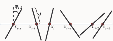
Figure 1: (Color online) Needle-shaped particles of length $2\ell$ and vanishing thickness are free to rotate in two dimensions, with their centers moving along a line. Particle (needle) $i$ is characterized by its translational position $x_{i}$ and orientation angle $\phi_{i}$.

Recently a formalism enabling direct calculation of elastic properties and stresses of a system of hard non-spherically-symmetric objects was developed mk by extending a previously known formalism for hard spheres fk . Not surprisingly, given that the elastic response in two and higher dimensions depends on a rank four tensor, the resulting expressions contain a large number of terms. Typical terms correspond to a variety of possible contacts between particles and numerous components of the separations between them (see, e.g., Eq. 23 in Ref. mk ). Since these expressions are obtained after numerous mathematical transformations, it is advisable to subject them to independent tests. Indeed they have been shown to reduce to the known results for isotropic objects, but up to now there had been no comparison with exact results for non-spherical particles. Here, we consider the statistical mechanics of a 1D system of hard needle-like particles rotating in two dimensions with their centers affixed to a 1D line, as depicted in Fig. 1. The needles are not allowed to intersect, and thus act as “hard” potentials. This model is a particular case of a group models considered by Lebowitz et al. lebowitz with anisotropic objects in one dimension. From the perspective of complexity, such systems are a slight generalization of the Tonks gas, yet they provide non-trivial insights into the interplay of rotational and translational degrees of freedom. The model can be solved exactly, and thermodynamic properties, such as elastic coefficients, can be calculated. We compare the values obtained analytically by the transfer matrix method, with those from MC simulations using the expressions from Ref. mk adapted to the 1D case.

The paper is organized as follows: The model of hard needles is introduced in Sec. II, and we demonstrate how the relative orientations of neighbors leads to an effective hard-potential as a function of their separation. Sec. III is devoted to reviewing how elastic properties of a system can be characterized, and the expressions for computing elastic coefficients in 1D are presented. The numerical difficulties associated with evaluation of various quantities by MC simulations are also described. In Sec. IV we present the transfer matrix method for solution of the model. Details of the MC simulation are presented in Sec. V, along with comparisons to results obtained by transfer matrix method. Discussion and additional features of the model are presented in Sec. VI.

II Model

Figure 1 depicts a configuration of our model, consisting of needles of length $2\ell$, with their center positions restricted to move on a 1D line. Needle $i$ is characterized by its position $x_{i}$, and orientation $\phi_{i}$ measured with respect to the normal to the line. Since orientations differing by $\pi$ are indistinguishable, we restrict $-\pi/2\leq\phi_{i}<\pi/2$. (Such entities, called directors, frequently appear in the description of liquid crystals degennes_liquid .) As $\ell$ is the only microscopic length scale in the problem, it can be used to construct dimensionless parameters. In particular, the mean distance between particles $a$ is made dimensionless by considering $a/\ell$, while the density $n$ can be replaced by $n\ell$.

The needles are not allowed to intersect but do not interact otherwise. Since the particles cannot cross each other, we number them (left-to-right) along the 1D line, and require that this order is unchanged, i.e. $x_{i-1}<x_{i}$. (This convention simplifies the enumeration of the possible contacts between particles.) Thus the distance of closest approach between adjacent needles is a function of their orientations, given $\ell d$, with the dimensionless function

$$d_{i-1,i}(\phi_{i-1},\phi_{i})=\frac{\sin|\phi_{i}-\phi_{i-1}|}{\max[\cos(\phi_{i-1}),\cos(\phi_{i})]}\,.$$ (1)

This function is depicted in Fig. 2, and varies between zero (when the needles are parallel, $\phi_{i}=\phi_{i-1}$) to 2 (with the needles lying on the line, $\phi_{i}=-\phi_{i-1}\to\pi/2$). Note that value of $d$ is poorly-defined at the points $(\pm\pi/2,\pm\pi/2)$, and depends on the limiting procedure. Analytic computations would have been considerably simplified if $d$ was only a function of the difference in orientation, but this is not the case because of the denominator in Eq. (1).

We consider a collection of $N$ needles, either in an ensemble of fixed length $L$ (for MC simulations), or fixed external pressure (force) $p$ (for transfer matrix studies). It is convenient to impose the boundary conditions through the definition of the minimal distance. For the MC simulations, we introduce fictitious particles $i=0$ an $i=N+1$. Periodic boundary conditions on a line of length $L$ are implemented by requiring $x_{N+1}=x_{1}+L$ and $\phi_{N+1}=\phi_{1}$, while $x_{0}=x_{N}-L$ and $\phi_{0}=\phi_{N}$. This extends the validity of Eq. (1) to $i=1$ and $i=N+1$, enabling the treatment of all particles on equal footing. In the fixed pressure ensemble, which is used in transfer matrix calculations, the orientation of the first (last) particle $i=1$ ($i=N$) is restricted only by its neighbor from the right (left), i.e. $i=2$ ($i=N-1$). The position of the both end particles is arbitrary in this ensemble, with $x_{1}>0$ and $x_{N}=L$ (which is also a variable in this ensemble). In this case, we set $d_{0,1}=d_{N,N+1}=0$.

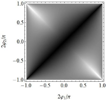
Figure 2: Gray-level representation of the function $d_{1,2}(\phi_{1},\phi_{2})$ in Eq. (1) for the dependence of minimal distance between needles on their orientations. The black diagonal corresponds to $d=0$ for parallel needles, while white corresponds to $d=2$ for needles along the line.

As explained above, adjacent particles interact via the hard potential

$$V_{i-1,i}\equiv V(x_{i}-x_{i-1},\phi_{i-1},\phi_{i})=$$

$$\begin{cases}0,&\text{if $x_{i}-x_{i-1}>\ell d_{i-1,i}$,}\\ \infty,&\text{otherwise.}\end{cases}$$ (2)

As such a potential does not have an energy scale, the temperature $T$ will appear only as a prefactor in the thermodynamic quantities. In particular, the Helmholtz free energy $F$ which is an extensive quantity with units of energy will have a form $F=Nk_{B}Th(n\ell)$, where $k_{B}$ is the Boltzmann constant. In 1D, the pressure $p$, and the elastic coefficient $C$ have units of force and can be made dimensionless by considering $f\equiv\beta p\ell$ and $\beta C\ell$, where $\beta=1/k_{B}T$. The Gibbs free energy $G=Nk_{B}Tg(f)$ depends only on the dimensionless pressure $f$.

III Elasticity of 1D

Shape and size deformations of objects are usually described by the strain tensor lanlif . In 1D this reduces to a scalar quantity $\eta$ which simply relates the distorted size of the system $L^{\prime}$ to its original size $L$ via $L^{\prime 2}=L^{2}(1+2\eta)$ etausage . (While this definition is slightly awkward in 1D, the use of squared distances between points is convenient because in higher dimensions it clearly separates trivial changes in geometry caused by rotations, and real deformations.) In 1D, for small $\eta$, the Helmholtz free energy can be expanded as

$$\frac{F(\eta)}{L}=\frac{F(0)}{L}-p\eta+\frac{1}{2}C\eta^{2}+\dots\,,$$ (3)

where $C$ is the elastic coefficient of the body. (Note, that the free energy on the left hand side (l.h.s.) of the equation is divided by the undistorted size of the system.) Consequently, $p$ and $C$ can be calculated from the first and second derivatives of $F$ with respect to $\eta$ at fixed $T$.

While the elastic properties are more naturally obtained from the Helmholtz free energy, we will also use the Gibbs free energy $G=F+pL$, in which the pressure is the (imposed) variable kardar . The system size $L$, or the mean inter-particle distance is then obtained from $a=\left.\partial(G/N)/\partial p\right|_{T}$, or in terms of dimensionless variables

$$\frac{a}{\ell}=\left.\frac{\partial(\beta G/N)}{\partial f}\right|_{T}\,.$$ (4)

Similarly, $C=-\left.a/\left(\frac{\partial a}{\partial p}\right|_{T}\right)+p$, and

$$\beta\ell C=-\frac{a}{\left.\frac{\partial a}{\partial f}\right|_{T}}+f\,.$$ (5)

Squire et al. shh developed a formalism for a direct calculation of elastic parameters from the correlation functions of particles. In this approach stress (pressure) and elastic moduli are related to thermal averages of products of various inter-particle forces and separations. This formalism was extended to hard potentials in Refs. fk ; mk . Since for hard potentials the forces vanish except when the particles touch, the results depend on various contact probabilities. In two and three dimensions the stress and the elastic constants are tensors, and the expressions involve averages over a variety of components. These results simplify in 1D, and in particular, the expression for stress [Eq. (22) in Ref. mk ] can be considerably simplified: If we denote the separation between two adjacent needles by $s_{i}=x_{i+1}-x_{i}$, they are in contact if the argument of $\Delta_{i}=\delta[s_{i}-\ell d_{i,i+1}(\phi_{i},\phi_{i+1})]$ vanishes. The dimensionless pressure then $f$ becomes

$$f=n\ell\left(1+\frac{1}{N}\sum_{i}\langle s_{i}\Delta_{i}\rangle\right).$$ (6)

The first term in this expression is simply the pressure of the ideal gas, while the second term can be easily recognized as the mean value of the product of the inter-particle separation and force, as appears in the virial theorem virtheorem . To evaluate Eq. (6), we need the probability that two particles ($i$ and $i+1$) with specified orientations ($\phi_{i}$ and $\phi_{i+1}$) touch each other.

Similarly, the elastic coefficient $C$ can be expressed as

$$\beta C\ell=n\ell\left[2+\frac{3}{N}\sum_{i}\langle s_{i}\Delta_{i}\rangle+\frac{1}{N}\left(\sum_{i}\langle s_{i}\Delta_{i}\rangle\right)^{2}\right.$$ (7)

$$\left.-\frac{2}{N}\sum_{i<j}\langle s_{i}s_{j}\Delta_{i}\Delta_{j}\rangle-\frac{1}{2N}\sum_{i}\langle(s_{i}^{2}+s_{i+1}^{2})\Delta_{i}\Delta_{i+1}\rangle\right].$$

The last two sums in the right hand side (r.h.s.) of Eq. (7) involve averages of products of $\Delta$s, i.e. they require knowledge of the joint probability density of two simultaneous contacts. The last sum involves cases when three particles $i$, $i+1$ and $i+2$ touch each other, while the preceding sum depends also on cases when two independent pairs are in contact, i.e. particle $i$ touches $i+1$, and a different particle $j$ ($>i+1$) touches $j+1$. The l.h.s. of Eq. (7) is an intensive quantity, while the third and the fourth terms on its r.h.s. contain $O(N^{2})$ terms. However, most of the terms appearing in these two sums can be grouped in pairs $\langle s_{i}\Delta_{i}\rangle\langle s_{j}\Delta_{j}\rangle-\langle s_{i}s_{j}\Delta_{i}\Delta_{j}\rangle$, which decay to zero when the distance between the pairs of particles exceeds the correlation length. All the averages appearing in Eqs. (6) and (7) can be calculated in MC simulations.

IV Transfer matrix approach

The partition functions of 1D models with short range interactions can be found analytically using a transfer matrix method baxter ; casey ; kardar . It convenient to consider the isobaric ensemble with fixed external pressure (force) $p$, such that (the configurational part of) the partition function is given by

$$Z_{G}=\int\prod_{i=1}^{N}dx_{i}\prod_{i=1}^{N}d\phi_{i}{\rm e}^{-\beta\sum_{i=1}^{N}V_{i-1,i}-\beta px_{N}}.$$ (8)

Since $x_{N}=\sum_{i}s_{i}$, we can change variables and perform integrations over the separations $s_{i}$ between adjacent particles. For the hard potential given by Eq. (II), this leads to

$$Z_{G} =(\beta p)^{-N}\int\prod_{i=1}^{N}\left(d\phi_{i}{\rm e}^{-\beta p\ell d_{i-1,i}(\phi_{i-1},\phi_{i})}\right)$$

$$=(\beta p)^{-N}\int\prod_{i=1}^{N}\left(d\phi_{i}D_{i-1,i}(f;\phi_{i-1},\phi_{i})\right),$$ (9)

where

$$D_{i-1,i}(f;\phi_{i-1},\phi_{i})\equiv{\rm e}^{-fd_{i-1,i}(\phi_{i-1},\phi_{i})}.$$ (10)

(According to the definition of $d$, all $D$ are identical, except for $D_{0,1}=D_{N,N+1}\equiv 1$ at the boundaries, as explained in the Sec. II.)

The expression in Eq. (1) is too complicated for the integrals in Eq. (IV) to be performed analytically. Nevertheless, multiple integrals of this kind can be easily performed numerically to any desired accuracy. We can subdivide the range of the angular integration into $M$ equal segments, by setting $\phi_{k}=-\pi/2+\frac{\pi}{M}k$, with $k=0,1,\cdots,M-1$. This replaces the function $D$ by an $M\times M$ matrix, and the integrals in Eq. (IV) are replaced by matrix products. The partition function then becomes

$$Z_{G}=(\beta p)^{-N}(\pi/M)^{N}\tilde{v}D^{N-1}v,$$ (11)

where $v$ is a column vector with all of its elements equal to 1. Repeated multiplications can be performed numerically, first multiplying $D$ by itself, then multiplying the resulting matrix by itself, etc.. After a total of $K$ such iterations we arrive at $D^{N}$, with $N=2^{K}+1$. The exponential dependence on $K$ allows us to achieve very large values of $N$, in practice we used $K=20$ in our simulations. For moderate pressures, the discretization of the angle $\phi$ has little influence on the result once $M$ exceeds 10, and we report results for $M=512$. (It should be noted, that the same results can also be obtained by numerically finding the largest eigenvalue of $D$. However, in our case this alternative provides no numerical advantage.) From the numerical value of $Z_{G}$, we then obtain the Gibbs free energy

Figure 3 depicts the scaled Gibbs free energy calculated by this numerical procedure. For non-interacting needles the partition function is $Z_{0}=(\pi/\beta p)^{-N}$, and the corresponding $\beta G_{0}/N=\ln(\beta p/\pi)$ is indicated by the lower line in the figure. (Both curves exclude the trivial contribution due to kinetic energy.)

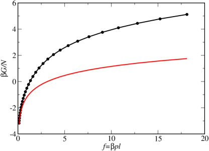
Figure 3: (Color online) The upper curve depicts the Gibbs free energy per particle (made dimensionless by multiplying by $\beta$) as a function of the dimensionless pressure $f=\beta p\ell$. The lower curve shows, for comparison, the same quantity for non-interacting needles; the curves begin to separate when $f$ is larger than about one.

V Simulations and results

A Monte Carlo procedure was used to evaluate the pressure and elastic coefficient of the system of hard needles. We simulated $N=128$ particles with periodic boundary conditions. Correlations between the needles for small and moderate densities do not persist past a few neighbors, and our choice of $N$ caused no perceptible finite size effects. An elementary MC move consists of randomly choosing a needle, randomly deciding whether to displace or to rotate it, and attempting to perform such a move. The move is accepted if in the new position, or with new orientation, the needle does not overlap with neighboring needles. The particles are sequentially ordered, and a position change is rejected if it changes this ordering. The attempted moves are uniformly distributed over an interval, whose width is chosen to be as large as possible, while maintaining an acceptance rate larger than 50%. The varying size of the interval implies a diffusion constant for each particle that decreases with increasing density. A single MC time unit consists of $2N$ attempts to move or rotate particles. The relaxation time of the system is proportional to $L^{2}$, and inversely proportional to the diffusion constant and elastic coefficient. (The latter increases with increasing density.) Our choice of elementary step ensured that, within the examined range of densities, the relaxation time was approximately constant and remained of order $N^{2}$. This was verified by directly measuring several autocorrelation functions. For every density $n$ the simulation time was $5\times 10^{5}N^{2}$. Such long times are required to ensure high accuracy of measured contact probabilities, as explained below.

The presence of the Dirac $\delta$-function in the definition of $\Delta_{i}$ necessitates delicate handling. Both Eq. (6) and Eq. (7) require measuring separation $s_{i}$ between the adjacent needles at the moment of contact. Such events have zero probability, and the formulas really involve probability densities. The latter can be evaluated by examining the probability that the two needles are within $\epsilon_{1}$, and divide the result by $\epsilon_{1}$. Of course, the number of such near collisions decreases with decreasing $\epsilon_{1}$, and the statistical error increases. The situation is even worse for terms of type $\langle s_{i}s_{j}\Delta_{i}\Delta_{j}\rangle$, where two simultaneous contacts are supposed to appear. One may define two near collision events by considering intervals of size $\epsilon_{1}$ and $\epsilon_{2}$. The opposing requirements of having $\epsilon_{i}\rightarrow 0$ (for accurate calculation of probability densities), and large $\epsilon_{i}$ (to ensure statistical accuracy) can be partially reconciled by considering each argument of a $\delta$-function being in the range $[m\epsilon,(m+1)\epsilon)$, with $m=0,1,\cdots,M$. We used $M=10$, and $\epsilon=0.002$ (0.01) for high (low) particle density simulations. With 11 data points for single contact terms, and $11^{2}$ points for two-contact terms, we could view the results as a function of one variable $m_{1}$, or two variables $m_{1}$ and $m_{2}$, and extrapolate the results to the “exact contact” limit. The accuracy and practicality of such a procedure has been demonstrated in Ref. fk . The total simulation time was determined by requirement of having sufficient number of terms in each “bin” of the statistical procedure explained above. The total simulation time was dictated by the need to have a very accurate estimate of the fourth term on the r.h.s. of Eq. (7).

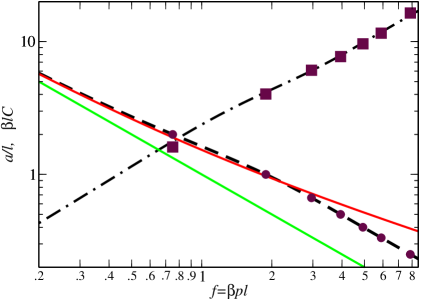
Figure 4: (Color online) The mean distance between particles $a$ (in units of $\ell$), as a function of dimensionless force $f$, for an ideal gas (lower continuous line) as compared with the virial expansion truncated at the second term (upper continuous line), and with the exact transfer matrix result (dashed line). The dashed-dotted line is the transfer matrix result for the elasticity coefficient $C$. Solid circles represent the relation between $a$ and $f$ from the MC simulations. Solid squares represent the MC results for the elastic coefficient.

Since the MC simulation is performed in the ensemble of fixed length, the density or mean inter-particle distance $a$ are given, while the dimensionless pressure $f$ and the dimensionless elastic modulus $\beta\ell C$ are calculated. The full circles in Fig. 4 depict the calculated dependence of $f$ (horizontal axis) on $a$ (vertical axis). The error bars on $f$ are negligible, since Eq. (6) includes only single pair contacts, and the large statistics as well as small $\epsilon_{1}$ ensures very high accuracy. This result is compared with the relation between $f$ and $a$ obtained from the Gibbs free energy via Eq. (4) by taking the numerical derivative of $G$ calculated by the transfer matrix method. The latter is depicted by the dashed line. Excellent agreement is obtained between the results from these two methods.

The solid squares in Fig. 4 depict the MC results for the dimensionless elastic coefficient $\beta\ell C$ (vertical axis), as a function of the dimensionless pressure $f$ (horizontal axis). Since in the MC procedure $f$ is itself a computed quantity, there are now also horizontal error bars, which are negligible as explained in the previous paragraph. The accuracy of $C$, however, is much lower and depends on both statistical errors, and systematic errors from extrapolation to the true contact probability densities. We chose the values of $\epsilon_{i}$, and the simulation time in such a way that both errors were of the same order. We estimate that the vertical error bars are approximately the size of the symbol for the leftmost point, and decrease to half the symbol size for the rightmost point. The dashed-dotted line depicts the same relation obtained from $G$ by using Eq. (5) and the transfer matrix calculations. The results from both approaches coincide within the estimated errors.

VI Discussion

The good agreement between the results from MC simulations, based on contact probabilities, and those from the transfer matrix method, support the validity of the expressions reproduced in Eqs. (6), (7) for the pressure and elastic moduli of hard potentials. While limited to 1D, this is the first direct comparison between formulae derived in Ref. mk , and an exact alternative approach.

We conclude by pointing out an interesting feature of the hard needle system: Both at small and large densities, the pressure and elastic coefficient are related by the simple expression $C=2p$, while the behavior at intermediate densities is more complicated. For low pressure (density) the system behaves as an ideal gas with $a=(\beta p)^{-1}$, and substituting in Eq. (5) immediately yields $C=2p$ in this limit. Interestingly, as discussed by Lebowitz et al. lebowitz , the relation between density and pressure also simplifies at very high pressure (density). In this limit the angular integrations are themselves constrained by pressure, and a Gaussian approximation leads to additional powers of $\beta p$ in the Gibbs partition function. This in turn leads to a density $n=a^{-1}=2\beta p$, i.e. the same functional dependence as an ideal gas but with a factor of 2. Inserting this limiting behavior into Eq. (5) again leads to $C=2p$ as in the ideal gas limit.

The lower solid line if Fig. 4 depicts the the dependence of $a$ on $f$ for an ideal gas. The curve deviates from ideal behavior for values of $f$ larger than about 1. At higher densities (and pressures) we can improve upon the ideal gas behavior by using a virial expansion. From the form of the interaction we compute a second virial coefficient of $B_{2}=8/\pi^{2}$. As indicated by the upper solid line in Fig. 4, inclusion of the second virial coefficient provides a good approximation for $f$ up to 3. Clearly there is no no simple relation between $C$ and $f$ in this intermediate region.

The focus of this paper was to use the model of hard needles to validate the relation between elastic moduli and contact probabilities for the exactly solvable model of hard needles. However, the model itself has some interesting features, which will be explored elsewhere kk_tbp . In particular the simplified behavior alluded above in the high density limit is related to an incipient critical point. The nature and universality of this criticality is related to the shapes of the hard objects (in this case, needles).

- (1) L. Tonks, Phys. Rev. 50, 955 (1936)
- (2) H. Takanishi, Proc. Phys.-Math. Soc. Japan 24, 60 (1942). (Reprinted in Mathematical Physics in One Dimension, ed. by E. H. Lieb and D. C. Mattis (Academic Press, New York, 1966), p. 25.
- (3) N. Metropolis, A. W. Rosenbluth, M. N. Rosenbluth, A. H. Teller and E. Teller, J. Chem. Phys. 21, 1087 (1953).
- (4) A. P. Gast and W. B. Russel, Phys. Today 51, 24 (1998).
- (5) W. G. Hoover and F. H. Ree, J. Chem. Phys. 49, 3609 (1968), and 47, 4873 (1967); B. J. Alder, W. G. Hoover, and D. A. Young, J. Chem. Phys. 49, 3688 (1968).
- (6) P. G. de Gennes and J. Prost, The Physics of Liquid Crystals, 2nd ed. (Oxford University Press, 1995).
- (7) L. Onsager, Ann. NY Acad. Sci. 51, 627 (1949).
- (8) D. Frenkel and R. Eppenga, Phys. Rev. Lett. 49, 1089 (1982); R. Eppenga and D. Frenkel, Mol. Phys. 52, 1303 (1984); M. A. Bates and D. Frenkel, Phys. Rev. E 57, 4824 (1998).
- (9) D. Frenkel and J. F. Maguire, Mol. Phys. 49, 503 (1983), and Phys. Rev. Lett. 47, 1025 (1981).
- (10) D. Fox, M. M. Labes and A. Weissberger, editors, Physics and Chemistry of Organic Solid State, vol. 1 (Interscience, New York, 1963).
- (11) M. Murat and Y. Kantor, Phys. Rev. E 74, 031124, 2006.
- (12) O. Farago and Y. Kantor, Phys. Rev. E 61, 2478, 2000
- (13) J. L. Lebowitz, J. K. Percus and J. Talbot, J. Stat. Phys. 49, 1221,1987.
- (14) L. D. Landau and E. M. Lifshits, Theory of Elasticity (Pergamon Press, Oxford, 1986).
- (15) T. H. K. Barron and M. L. Klein, Proc. Phys. Soc. 85, 523 (1965).
- (16) M. Kardar, Statistical Physics of Particles (Cambridge University Press, Cambridge, 2007).
- (17) D. R. Squire, A. C. Holt and W. G. Hoover, Physica 42, 388 (1969).
- (18) R. K. Pathria, Statistical Mechanics, 2nd ed. (Butterworth-Heinemann, Oxford, 1996); M. Toda, R. Kubo, and N. Saito, Statistical Physics: Equilibrium Statistical Mechanics Part I (Springer, Berlin, 1998); R. Balescu, Equilibrium and Nonequilibrium Statistical Mechanics (Wiley, New York, 1975).
- (19) R. J. Baxter, Exactly Solved Models in Statistical Mechanics (Academic Press, London, 1982).
- (20) L. M. Casey and L. K. Ryunnels, J. Chem. Phys. 51, 5070, 1968.
- (21) Y. Kantor and M. Kardar, to be published.