Development of General Relativistic Magnetohydrodynamic Code and its Application to Central Engine of Long Gamma-Ray Bursts

Abstract

In order to investigate formation of relativistic jets at the center of a progenitor of a long gamma-ray burst (GRB), we develop a two-dimensional general relativistic magnetohydrodynamic (GRMHD) code. We show the code passes many, well-known test calculations, by which the reliability of the code is confirmed. Then we perform a numerical simulation of a collapsar using a realistic progenitor model. It is shown that a jet is launched from the center of the progenitor. We also find that the mass accretion rate after the launch of the jet shows rapid time variability that resembles to a typical time profile of a GRB. The structure of the jet is similar to the previous study: a poynting flux jet is surrounded by a funnel-wall jet. Even at the final stage of the simulation, bulk Lorentz factor of the jet is still low, and total energy of the jet is still as small as $10^{48}$ erg. However, we find that the energy flux per unit rest-mass flux is as high as $10^{2}$ at the bottom of the jet. Thus we conclude that the bulk Lorentz factor of the jet can be potentially high when it propagates outward. It is shown that the outgoing poynting flux exists at the horizon around the polar region, which proves that the Blandford-Znajek mechanism is working. However, we conclude that the jet is launched mainly by the magnetic field amplified by the gravitational collapse and differential rotation around the black hole, rather than the Blandford-Znajek mechanism.

1. Introduction

Gamma-Ray Bursts (GRBs; in this study, we consider only long GRBs, so we refer to long GRBs as GRBs hereafter) have been mysterious phenomena since their discovery in 1969 Klebesadel et al. (1973). Last decade, observational evidence for supernovae (SNe) and GRBs association has been reported (e.g. Woosley and Bloom 2006, and references therein).

Some of the SNe that associate with GRBs were very energetic and blight. The estimated explosion energy was of the order of $10^{52}$ ergs, and produced nickel mass was $\sim 0.5M_{\odot}$. Thus they are categorized as a new type of SNe (sometimes called as hypernovae). The largeness of the explosion energy is very important, because it can not be explained by the standard core-collapse SN scenario, and other mechanism should be working at the center of the progenitors.

The promising scenarios are the collapsar scenario Woosley (1993) and the magnetar scenario (Usov, 1992). In the collapsar scenario, a rapidly rotating black hole (BH) is formed at the center, while a rapidly rotating neutron star with strong magnetic fields ($\sim 10^{15}$G) is formed in the magnetar scenario. Many numerical simulations have been done for the collapsar scenario (MacFadyen & Woosley, 1999; Proga et al., 2003; Proga & Begelman, 2003; Mizuno et al. 2004a, ; Mizuno et al. 2004b, ; Proga, 2005; Fujimoto et al., 2006; Shibata et al., 2006; Nagataki et al., 2007; Sekiguchi & Shibata, 2007; Suwa et al., 2007; Barkov & Komissarov 2008a, ) and the magnetar scenario (Takiwaki et al., 2004; Komissarov & Barkov, 2007; Burrows et al., 2007; Bucciantini et al., 2008; Dessart et al., 2008; Takiwaki et al., 2008; Bucciantini et al., 2009). In this study, we investigate the collapsar scenario.

In the collapsar scenario, a BH is formed as a result of gravitational collapse. Also, rotation of the progenitor plays an essential role. Due to the rotation, an accretion disk is formed around the equatorial plane. On the other hand, the matter around the rotation axis falls into the BH almost freely. It is pointed out that the jet-induced explosion along the rotation axis may occur due to the heating through pair annihilation of neutrinos and anti-neutrinos that are emitted from the accretion disk (Woosley, 1993; MacFadyen & Woosley, 1999; Fryer & M$\rm\acute{e}$sz$\rm\acute{a}$ros, 2000). Effect of extraction of rotation energy from the accretion disk by magnetic field lines that leave the disk surface (Blandford-Payne effect Blandford & Payne (1982)) is also investigated by several authors (Proga et al., 2003; Proga & Begelman, 2003; Mizuno et al. 2004a, ; Mizuno et al. 2004b, ; Proga, 2005; Fujimoto et al., 2006; Nagataki et al., 2007; Suwa et al., 2007). Recently, the effect of extraction of rotation energy from the BH through outgoing poynting flux (Blandford-Znajek effect Blandford & Znajek (1977)) is investigated Barkov & Komissarov 2008a . In order to investigate the collapsar scenario completely, a high-quality numerical code including effects of a lot of microphysics (neutrino physics, nuclear physics, and equation of state for dense matter) and macrophysics (magneto-hydrodynamics, general relativity) has to be developed. Although many numerical studies have been reported, such a numerical code has not been developed yet. Thus we have to develop our numerical code step by step.

In this study, we investigate the dynamics of collapsars taking into account the general relativistic effects. Extraction of rotation energy from a rotating BH is one of them. Also, even when the rotation energy is extracted from the accretion disk, the properties of the accretion disk should depend on the properties of the BH: if the BH is rotating, the inner region of the accretion disk should be enforced to co-rotates with the BH. We investigate how a jet is launched at the center of a progenitor, and how the property of the jet is. Effects of rotation of the BH on the formation of GRB jet have not been investigated so much. Barkov and Komissarov (2008) is a pioneering study. However, only one case is investigated in their study, and the initial progenitor model they used is a simplified one-dimensional model without rotation and magnetic fields Bethe (1990). Since there should be many initial conditions of progenitors (progenitor mass, metallicity, angular momentum, magnetic fields), it should be important to investigate the general relativistic effects using a different initial condition from the previous study. In this study, we use a realistic initial condition for the progenitor model that is developed by Woosley and Heger (2006), in which rotation and magnetic fields are taken into account.

When we investigate the general relativistic effects, one has to develop a General Relativistic Magneto-Hydro Dynamic (GRMHD) code. So far, there are many studies on GRMHD code for fixed background space times using high-order conservative schemes based on either approximate or full wave-decomposition Riemann solvers (Gammie et al., 2003; Komissarov, 2005; Anninos et al., 2005; Ant$\rm\acute{o}$n et al., 2006; Del Zanna et al., 2007; Tchekhovskoy et al., 2007) or non-conservative schemes (De Villiers & Hawley, 2003; Anninos et al., 2005). Since the accreted mass onto the BH is still less than the initial BH mass in this study, we take the GRMHD code for the fixed background. Especially, we develop our code using the conservative scheme of Gammie et al. (2003) with the method of Noble et al. (2006) for transforming conserved variables to primitive variables.

The plan of the paper is as follows. In section 2, we present the formulation of the GRMHD code. In section 3, we show results of many, well-known test calculations to confirm the reliability of the code. After we show the reliability, we present results of numerical simulations of collapsars in section 4. Summary and discussion are presented in section 5.

2. Development of GRMHD Code

We have developed a two-dimensional GRMHD code following Gammie et al. (2003) and Noble et al. (2006). We have adopted a conservative, shock-capturing scheme with Harten, Lax, and van Leer (HLL) flux term Harten et al. (1983) with flux-interpolated constrained transport technique T$\rm\acute{o}$th (2000). We use a third-order Total Variation Diminishing (TVD) Runge-Kutta method for evolution in time, while monotonized central slope-limited linear interpolation method is used for second-order accuracy in space van Leer (1977). 2D scheme (2-dimensional Newton-Raphson method) is usually adopted for transforming conserved variables to primitive variables Noble et al. (2006).

When we perform simulations of GRMHD, Modified Kerr-Schild coordinate is basically adopted with mass of the BH ($M$) fixed where the Kerr-Schild radius $r$ is replaced by the logarithmic radial coordinate $x_{1}=\ln r$. When we show the result, the coordinates are sometimes transfered from Modified Kerr-Schild coordinate to Kerr-Schild one for convenience. In the following, we use $G=M=c=1$ unit. $G$ is the gravitational constant, $c$ is the speed of light, and $M$ is the gravitational mass of the BH at the center. Throughout this paper we follow the standard notation Misner et al. (1970).

2.1. Formalism

Number of variables that appear in the equations of GRMHD is 13: rest-mass density ($\rho$), internal energy density ($u$), pressure ($p$), four-velocity of fluid ($u^{\mu}$), and Faraday tensor ($F^{\mu\nu}$). Note that Faraday tensor has only 6 independent components due to the relation $F^{\mu\nu}=-F^{\nu\mu}$. We can reduce the number of independent variables to 8 using the MHD condition ($u_{\mu}F^{\mu\nu}=0$), equation of state ($p=(\gamma-1)u$: $\gamma$-law gas is assumed), and the unit length of the four velocity ($u_{\mu}u^{\mu}=-1$). Note that the number of independent equations of the MHD condition is 3. We choose ($\rho$,$u$,$u^{i}$,$B^{i}$) as the 8 independent variables where $u^{i}$ is the space component of the four velocity. $B^{i}$ can be written as $\Re^{i}$/$\alpha$ where $\alpha$ is the lapse function ($\alpha=\sqrt{-1/g^{tt}}$) and $\Re^{i}$ is the magnetic field measured by the Fiducial observer (FIDO) whose four velocity is $n_{\mu}=(-\alpha,0,0,0)$. We call these independent variables as the primitive variables. Below, we introduce the conserved variables. Of course, number of the conserved variables is also 8. Thus we require 8 basic equations to follow the time evolution of the system.

The basic equations of GRMHD represent the rest-mass conservation, the energy-momentum conservation, and space component of the induction equation that determines the time evolution of the magnetic fields. These are:

$$\partial_{t}(\sqrt{-g}\rho u^{t})=-\partial_{i}(\sqrt{-g}\rho u^{i})$$ (1)

$$\partial_{t}(\sqrt{-g}T^{t}_{\nu})=-\partial_{i}(\sqrt{-g}T^{i}_{\nu})+\sqrt{-g}T^{\kappa}_{\lambda}\Gamma^{\lambda}_{\nu\kappa}$$ (2)

$$\partial_{t}(\sqrt{-g}B^{i})=-\partial_{j}\left[\sqrt{-g}(b^{i}u^{j}-b^{j}u^{i})\right],$$ (3)

where $T^{\mu\nu}$ is the stress energy tensor that is composed of the sum of the matter part ($T^{\mu\nu}_{\rm Matter}=(\rho+u+p)u^{\mu}u^{\nu}+pg^{\mu\nu}$) and electromagnetic part ($T^{\mu\nu}_{\rm EM}=F^{\mu\alpha}F^{\nu}_{\alpha}-g^{\mu\nu}F_{\alpha\beta}F^{\alpha\beta}/4$). The factor of $\sqrt{4\pi}$ is absorbed into the definition of the Faraday tensor Gammie et al. (2003). $b^{\mu}$ is introduced so that Eq.(3) looks simple, and it is defined as $b^{\mu}=\epsilon^{\mu\nu\kappa\lambda}u_{\nu}F_{\lambda\kappa}$ where $\epsilon^{\mu\nu\kappa\lambda}=(-1/\sqrt{-g})\left[\mu\nu\lambda\kappa\right]$. $\left[\mu\nu\lambda\kappa\right]$ is the completely antisymmetric symbol. In the fluid-rest frame, $b^{\mu}$ becomes (0,$B^{i}$).

In this study, we adopt the conservative scheme for integration of the GRMHD equations. In this case, the left terms of Eq.(1)-(3) are considered to be fundamental variables and called as the conserved variables. The right terms of Eq.(1)-(3) are flux terms with a source term (the second right term of Eq.(2)).

Since we have to estimate pressure of the fluid, we have to estimate the primitive variables from the conserved variables at each time step. The problem is that the primitive variables can not be expressed analytically by the conserved variables. Thus we have to use the Newton-Raphson method to obtain the primitive variables from the conserved ones Noble et al. (2006).

Basically, we adopt the 2D scheme introduced by Noble et al. (2006) to calculate the primitive variables. However, it sometimes happens that the 2D scheme fails to converge well, and the primitive variables can not be obtained precisely. In such a case, we first adopt the 1$\rm D_{W}$ scheme introduced by Noble et al. (2006) and see whether the 1$\rm D_{W}$ scheme converges. If it converges well, we adopt the primitive variables obtained by the 1$\rm D_{W}$ scheme for the next time step. Otherwise, we adopt the second choice explained in the following subsection.

2.2. Supplemental Method to Calculate Primitive Variables

Following Noble et al. (2006), we introduce convenient variables $v^{2}$, $W$, $Q^{\mu}$, and $\bar{Q}^{\mu}$. These variables, of course, depend on the primitive variables. The definition of these variables are: $v^{2}=v_{i}v^{i}$, $W=\omega\Gamma^{2}$, $Q^{\mu}=\alpha T^{t\mu}$, and $\bar{Q}^{\mu}$ = $j^{\mu}_{\lambda}Q^{\lambda}$, where $v^{i}$ is the fluid velocity relative to FIDO, $\omega=\rho+u+p$, $\Gamma=1/\sqrt{1-v^{2}}$, and $j_{\mu\lambda}=g_{\mu\lambda}+n_{\mu}n_{\lambda}$. It is apparent that $Q^{\mu}$ and $\bar{Q}^{\mu}$ can be written analytically by the conserved variables. On the other hand, $v^{2}$ and $W$ can not be expressed analytically by the conserved variables. Thus, we have to solve $v^{2}$ and $W$ numerically in order to determine the proper, corresponding primitive variables.

Here we show that an upper limit and a lower limit for $W$ can be obtained before searching for a solution of $W$ and $v^{2}$ numerically. Thanks to this fact, all we have to do is to seek the solution with the condition $W_{\rm min}\leqq W\leqq W_{\rm max}$. From Eq.(28) and Eq.(29) in Noble et al. (2006), $W$ and $v^{2}$ satisfy the following equations:

$$v^{2}_{\rm eq28}=\frac{\bar{Q}^{2}W^{2}+(Q_{\mu}\Re^{\mu})^{2}(\Re^{2}+2W)}{(\Re^{2}+W)^{2}W^{2}}$$ (4)

$$v^{2}_{\rm eq29}=\frac{2}{\Re^{2}}\left[\frac{(Q_{\mu}\Re^{\mu})^{2}}{2W^{2}}-W+p-(Q_{\mu}n^{\mu})\right]-1.$$ (5)

From these equations and the relation $0\leqq v^{2}<1$, $v^{2}$ and $W$ satisfy the following relations:

$$f(W) = W^{4}+2\Re^{2}W^{3}+(\Re^{4}-\bar{Q}^{2})W^{2}-2(Q_{\mu}\Re^{\mu})^{2}W$$ (6)

$$- \Re^{2}(Q_{\mu}\Re^{\mu})^{2}\geqq 0$$

$$g(W)=W^{3}+\{\frac{1}{2}\Re^{2}+(Q_{\mu}n^{\mu})-p\}W^{2}-\frac{1}{2}(Q_{\mu}\Re^{\mu})^{2}\leqq 0$$ (7)

$$h(W)=W^{3}+\{\Re^{2}+(Q_{\mu}n^{\mu})-p\}W^{2}-\frac{1}{2}(Q_{\mu}\Re^{\mu})^{2}\geqq 0.$$ (8)

Since $f(0)\leqq 0$, $f^{{}^{\prime}}(0)\leqq 0$, and at least one of the solution for $f^{{}^{\prime\prime}}(W)=0$ is less than 0, there is only one positive solution $W_{a}$ that satisfies $f(W_{a})=0$. Thus, from Eq.(6), $W$ has to be greater than $W_{a}$.

We can understand the behavior of $g(W)$ from its first derivative for $W$:

$$g^{{}^{\prime}}(W)=W\left[3W+2\{\frac{1}{2}\Re^{2}+(Q_{\mu}n^{\mu})-p\}\right].$$ (9)

It is apparent that $W=0$ is a solution for $g^{{}^{\prime}}(W)=0$. As for the other solution(s), it is not so obvious because the pressure $p$ depends on $W$ and $v^{2}$. However, it will be natural to consider that the monotonic relation holds between $W$ and $p$. It means that the pressure rises when $W$ becomes larger. If this assumption is adopted, as long as $g^{{}^{\prime}}(W)=0$ has another solution, it is a positive one $W=W_{\alpha}\geqq 0$. This is because when $W=0$, $p$ should be also 0 and $\left[3W+2\{1/2\Re^{2}+(Q_{\mu}n^{\mu})-p\}\right]$ is a positive value. Thus, $g(W)=0$ has only one positive solution $W_{b}$. This holds even if $g^{{}^{\prime}}(W)=0$ has only one solution at $W=0$. Also, same conclusion can be derived for $h(W)$: there is only one positive solution $W_{c}$ that satisfies $h(W_{c})=0$.

Since $h(W)\geqq g(W)$, the relation $W_{c}\leqq W_{b}$ holds. In conclusion, $W$ has to be in the range $W_{\rm min}={\rm Max}(W_{a},W_{c})\leqq W\leqq W_{b}=W_{\rm max}$. Thus all we have to do is to find a solution of $W$ that satisfies $v^{2}_{\rm eq28}=v^{2}_{\rm eq29}$ in this range. This procedure is more expensive than the 2D scheme and the 1$\rm D_{W}$ scheme, but the solution for $W$ and $v^{2}$ is more likely to be found because the range for the solution of $W$ is determined apriori. Thus we use this method as a supplementary one to obtain the primitive variables.

Figure 1.— Simulation of 1D shock tube test (Komissarov 1999). The state at $t=1.0$ is shown in the figure. Number of grid points is 600. The calculation region is set to be $-2\leq x\leq 2$. The upper left panel shows density, the upper right panel shows pressure, the lower left panel shows the velocity in the x-direction, and the lower right panel shows the bulk Lorentz factor.

Figure 2.— Simulation of 1D collision test (Komissarov 1999). The state at $t=1.2$ is shown in the figure. Number of grid points is 600. The calculation region is set to be $-2\leq x\leq 2$. The left panels show density, velocity in the x-direction, and bulk Lorentz factor (from top to bottom), while right panels show pressure, velocity in x-direction, and y-component of magnetic field (from top to bottom).

3. Test Calculations

Using the GRMHD code that is developed in this study, we check whether it can pass many, well-known test calculations. The first three tests are special relativistic hydrodynamic (SRHD) or special relativistic magnetohydrodynamic (SRMHD) calculations, while the rest of three tests are GRMHD ones.

3.1. Shock Tube Problems

1D shock tube tests are the most basic test problems for SRHD/SRMHD. We have carried out a number of the test simulations introduced in Komissarov (1999) and Balsara (2001). Here we describe only two of them. One is the shock tube test1 and the other is the collision test (Komissarov, 1999; Mizuno et al., 2006). The initial left and right states are summarized in Table.1. Number of grid points is 600 for both simulations. The results are shown in Fig.1 and Fig.2, which show that the test calculations are well solved as in the previous studies.

3.2. Double Shock Problems

Here 2D shock tube problem is done to confirm whether the shock dynamics in the multidimensional flow can be solved safely. This problem includes the interactions of shocks, rarefactions, contact discontinuities. Initially a square computational domain is prepared in x-y plane and divided into four quarter boxes. Initial condition in each box is summarized in Table.2. This condition is same with previous study (Del Zanna & Bucciantini, 2001; Zhang & MacFadyen, 2006; Mizuta et al., 2006). We use 400$\times$400 uniform grid points in a square computational box. Boundary condition is open ones. Density contour at the final stage of the simulation is shown in Fig.3, which shows that our code reproduces the previous studies very well.

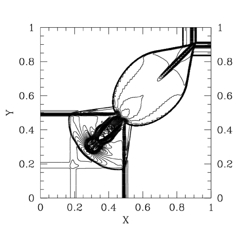
Figure 3.— Simulation of 2D shock tube problem. Density contour at $t=0.4$ is shown in the figure. Numbers of grid points are 400$\times$400. The calculation region is set to be $0\leq x\leq 1$ and $0\leq y\leq 1$.

3.3. Cylindrical Explosion Test

Here we go to a SRMHD test. A famous, cylindrical blast explosion test is done (Del Zanna et al., 2003; Leismann et al., 2005). We use the $[0,1]\times[0,1]$ Cartesian grid with a resolution of $N_{x}=N_{y}=250$ grid points. We define an initially static background with $\rho=1.0,p=0.01$, and $B_{x}=4.0$. The relativistic flow comes out by setting a much higher pressure, $p=10^{3}$ within a circle of radius $r=0.08$ placed at the center of the domain. $\gamma$ for the equation of state is set to be 4/3. Final time is set to be 0.4. The result is shown in Fig.4. The upper left panel shows the density contour in logarithmic scale. The upper right panel shows the pressure contour in logarithmic scale. The lower left panel shows contour of the bulk Lorentz factor. The lower right panel shows the divergence of the magnetic fields in logarithmic scale with magnetic field lines. These results are consistent with the previous studies. Especially, the divergence of the magnetic fields is kept as small as $10^{-14}$.

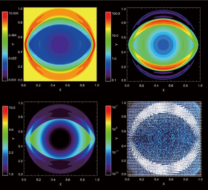
Figure 4.— A RMHD 2D cylindrical explosion test with a pressure jump as high as $10^{5}$. The state at $t=0.4$ is shown in the figure. Numbers of grid points are 250$\times$250. The calculation region is set to be $0\leq x\leq 1$ and $0\leq y\leq 1$. The upper left panel shows the density contour in logarithmic scale. The upper right panel shows the pressure contour in logarithmic scale. The lower left panel shows contour of the bulk Lorentz factor. The lower right panel shows divergence of the magnetic fields in logarithmic scale with magnetic field lines.

3.4. Gammie’s Flow

Next we consider a GRMHD test. A steady, magnetized inflow solution on the equatorial plane around a Kerr BH is considered (Takahashi et al., 1990; Gammie, 1999). Initially, the steady inflow solution for the Kerr parameter $a=0.5$ and the magnetization parameter $F_{\theta\phi}=0.5$ is set, and time evolution of the system is followed by the GRMHD code. In this calculation, Boyer-Lindquist coordinate is used. The calculation region is set to be [2.0 $\leqq r\leqq$ 4.04] and [$0.5-10^{-3}\leqq\theta/\pi\leqq 0.5+10^{-3}$]. The model is run for $t=1.5$. The physical values at boundaries are fixed throughout the simulation. Results are shown in Fig.5: density, radial component of the 4-velocity, the $\phi$ component of the 4-velocity, and $\Re^{\phi}$ at the final stage of the simulation. When the initial state is written in the same figure, we can see that the final state coincides with the initial state. To show it more quantitatively, we introduce the norms of the errors for these values as a function of the number ($N$) of grid points in the radial coordinate. The definition of the norm of the error is $\Sigma_{i=1}^{i=N}\left|a({\rm final})-a({\rm initial})\right|/\Sigma_{i=1}^{i=N}\left|a({\rm initial})\right|$. In Fig.6, the norms of errors are shown. We can see that these values converge roughly proportional to $N^{-2}$, as expected.

3.5. Blandford-Znajek Monopole Solution

Further we continue to test the GRMHD code. We consider the Blandford-Znajek monopole solution Blandford & Znajek (1977). This analytic solution has been investigated numerically by previous studies (Komissarov 2004b, ; McKinney & Gammie, 2004; Tanabe & Nagataki, 2008).

The computational domain is axisymmetric, with a grid that extends from $r_{\rm in}=0.98r_{+}$ to $r_{\rm out}=230$ and from $\theta=0$ to $\theta=\pi$ where $r_{+}=1+\sqrt{1-a^{2}}$ is the outer event horizon. The numerical resolution is 300 $\times$ 300. As an initial condition, we put the 0th order terms of the monopole solution around the BH Komissarov 2004b . That is, $\Re^{\mu}=-n_{\nu}^{*}F^{\mu\nu}=(0,\alpha\sin\theta/\sqrt{-g},0,0)$ in the Kerr-Schild coordinate where ${}^{*}F^{\mu\nu}$ and $g$ are the dual field tensor and determinant of the Kerr-Schild metric. The plasma velocity relative to the FIDO is set to zero initially, and its pressure and density are set to small value ($P=\rho=\Re^{2}/100$) so that the system becomes Force-Free like. Also, to keep the magnetization reasonably low, when the critical condition $0.01B^{2}\geq\Gamma^{2}\rho+(\gamma\Gamma^{2}-(\gamma-1))u$ is satisfied, density and internal energy are increased by the same factor so that the critical condition holds Komissarov 2004b . $\gamma$ is set to be 4/3. We have performed numerical simulations with the Kerr parameters 0, 0.01, 0.1, 0.2, 0.3, 0.4, 0.5, 0.6, 0.7, 0.8, 0.9, 0.95, 0.99, and 0.995 until time $t$ = 200.

Figure 5.— Gammie’s equatorial inflow solution in the Kerr metric with $a=0.5$ and magnetization parameter $F_{\theta\phi}=0.5$. Number of grid point is 1024. The state at $t=1.5$ is shown in the figure. The panels show density, radial component of the 4-velocity, the $\phi$ component of the 4-velocity, and $\Re^{\phi}$ at the final stage of the simulation. Boyer-Lindquist coordinate is used for the simulation.

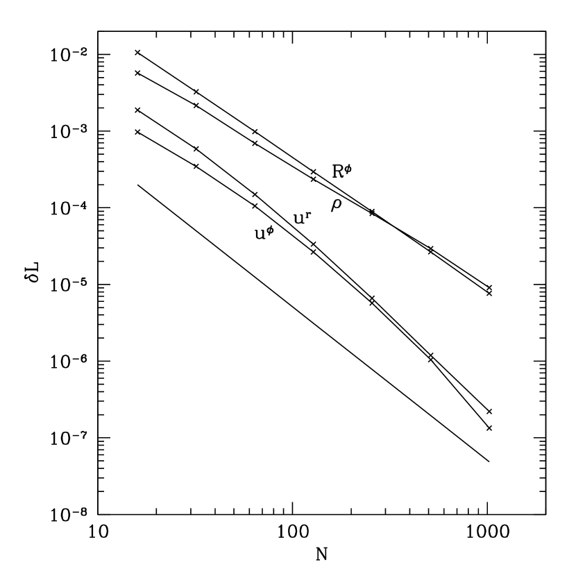
Figure 6.— Convergence results for the Gammie’s equatorial inflow solution in the Kerr metric with $a=0.5$ and magnetization parameter $F_{\theta\phi}=0.5$. Norms of the error for $\rho$, $u^{r}$, $u^{\phi}$, and $\Re^{\phi}$ at the final stage of the simulation are shown in the figure. The straight line represents the slope expected for second-order convergence. The definition of the norm of the error is written in the text.

Figure 7.— Outgoing poynting fluxes as a function of the zenith angle for the Blandford-Znajek monopole solution with Kerr parameter $a=0.01,0.1,0.15,0.2,0.3,0.4,0.5,0.6,0.7,0.8,0.9$, and $0.95$. The fluxes are measured at $r=20$ and $t=200$. Numbers of grid point are 300$\times$300.

The total energy flux, which is the integrated outgoing poynting flux over the zenith angle, can be written as

$$\dot{E} = 2\pi\int_{0}^{\pi}d\theta\sqrt{-g}(-T^{r}_{t})=2\pi\int_{0}^{1}dx_{2}\left(\frac{d\theta}{dx_{2}}\right)\sqrt{-g}(-T^{r}_{t})$$ (10)

$$= 2\pi\int_{0}^{1}dx_{2}F_{E},$$

where $x_{2}=\theta/\pi$ is introduced as a convenient variable Gammie et al. (2003).

In Fig.7, the outgoing poynting fluxes ($F_{E}$) as a function of zenith angle are shown. The fluxes are measured at $r=20$ at the final stage of the simulations. We would like to note that the outgoing poynting flux hardly depends on the radius where it is evaluated. This means that the conservation of the outgoing poynting flux is confirmed numerically.

In Fig.8(a), we plot the total energy flux ($\dot{E}$) at the final stage for small Kerr parameters ($0\leq a\leq 0.2$) by rectangular points. Dashed line is just the interpolation of the calculated values. For comparison, the second-order analytical solution is shown by dotted line and the forth-order analytical solution is shown by solid line. From this comparison, we can see that all of them coincide with each other. Thus the results of the numerical simulations by the GRMHD code are confirmed by analytical solutions.

The situation becomes different for large Kerr parameters. In Fig.8(b), we plot the same values with Fig. 8(a), but for wide range of the Kerr parameters ($0\leq a\leq 1$). We can see clearly the difference among three cases. This is because the analytical solution is obtained by the perturbation method in Kerr parameter, and it is applicable only for small Kerr parameters. Of course, there is no such limitation for the numerical simulations. Thus the total energy flux obtained by the numerical simulation is more reliable than the analytical estimation (see Tanabe and Nagataki (2008) for detailed discussion).

Figure 8.— Upper panel (a): Comparison of the derived, conserved, total energy flux. Dashed line with rectangular points is numerical result for small Kerr parameter ($0\leq a\leq 0.2$), dotted line shows the second-order analytical solution, and solid line represents the forth-order analytical solution. Lower panel (b): Same with upper panel, but for wide range of the Kerr parameters $(0\leq a\leq 1)$. Simulations are done for the Kerr parameters 0, 0.01, 0.1, 0.2, 0.3, 0.4, 0.5, 0.6, 0.7, 0.8, 0.9, 0.95, 0.99, and 0.995 until $t=200$.

3.6. Fishbone and Moncrief’s Test

Here we present a final test of the GRMHD code. A steady and stationary torus (Fishbone & Moncrief, 1976; Abramowicz et al., 1978) around a Kerr BH that is supported by both centrifugal force and pressure is solved numerically. Of course, it should be solved as a steady and stationary state.

We have integrated a Fishbone-Moncrief solution around a Kerr BH with $a=0.9$. We set $u^{t}u_{\phi}=4.45$ and $R_{\rm in}=6.0$. The grid extends radially from $r_{\rm in}=1.40$ to $r_{\rm out}=100$. The same floors with Gammie et al. (2003) are used for $\rho$ and $u$. The numerical resolution is $N\times N$ and the solution is integrated for $t=10$. The resulting norm of the error, which converges roughly proportional to $N^{-2}$, is shown in Fig.9.

Next we follow the time evolution of the Fishbone-Moncrief solution with magnetic fields. The vector potential, $A_{\phi}\propto{\rm max}(\rho/\rho_{\rm max}-0.2,0)$ where $\rho_{\rm max}$ is the peak density in the torus, is introduced Gammie et al. (2003). The field is normalized so that the minimum value of $p_{\rm gas}/p_{\rm mag}$ becomes $10^{2}$. The time integration extends for $t=2000$. The number of grid points is $256\times 256$, and the grid extends radially from $r_{\rm in}=1.40$ to $r_{\rm out}=300$ while it extends in the zenith angle from $\theta=0$ to $\theta=\pi$.

The density contours in logarithmic scale (from $10^{-6}$ to $10^{3}$) are shown in Fig.10. These are projected on the (r sin $\theta$,r cos $\theta$)-plane. The upper left panel shows the initial state. The upper right panel shows the final state of the simulation without magnetic fields. The lower left panel shows the final state of the simulation with magnetic fields. The lower right panel is same with the lower left one, but for a wide region. Due to the presence of the magnetic fields, the angular momentum in the torus is conveyed outward and the the torus starts to accrete, and the jet is launched from the BH around the polar region. This result is consistent with the previous studies (Gammie et al., 2003; McKinney & Gammie, 2004; McKinney 2006a, ; Mckinney 2006b, ).

Figure 9.— Convergence results for the Fishbone-Moncrief problem for a Kerr BH with $a=0.9$. The straight line represents the slope expected for second-order convergence. Kerr-Schild coordinate is used for the simulation.

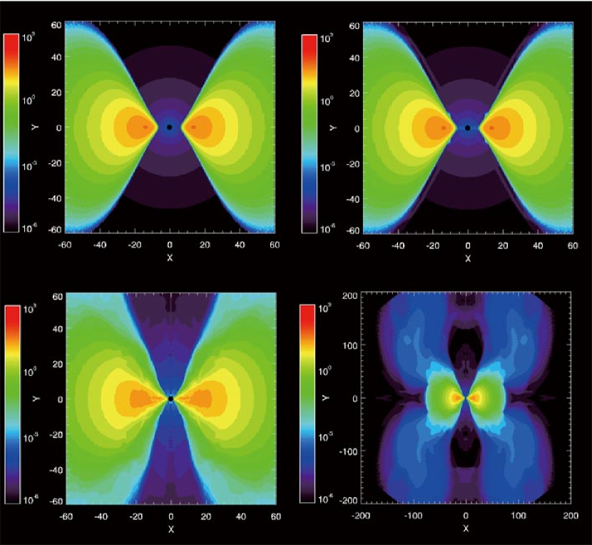
Figure 10.— Density contour in logarithmic scale (from $10^{-6}$ to $10^{3}$) for the Fishbone-Moncrief problem for the Kerr parameter $a=0.9$. Number of grid points is $256\times 256$. The simulations are done until $t=2000$. The upper left panel shows the initial state. The upper right panel shows the final state of the simulation without magnetic fields. The lower left panel shows the result with magnetic fields. The lower right panel is same with the lower left one, but for a wide region. These results are projected on the (r sin $\theta$,r cos $\theta$)-plane.

4. Simulation of Collapsar

Since our code has passed the many test calculations shown in the previous section, we now simulate the dynamics of a collapsar using the code. However, we have to say beforehand that no microphysics is included in the code such as nuclear reactions, neutrino processes, and equation of state for dense matter. So this is the FIRST STEP of our project to simulate the dynamics of a collapsar and formation of a relativistic jet of a GRB.

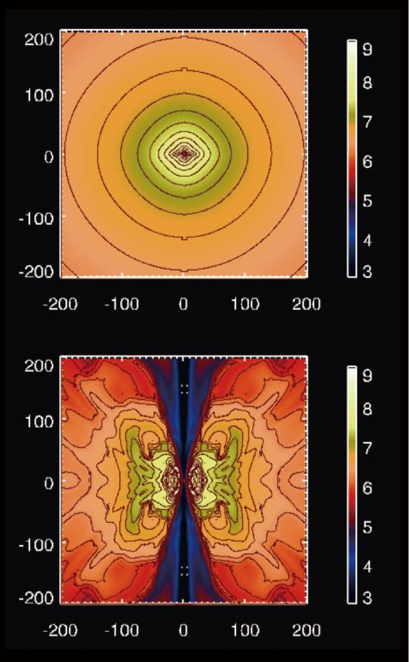
Figure 11.— Contours of rest mass density at the central region in logarithmic scale, in which cgs units are used assuming that the gravitational mass of the BH is 2$M_{\odot}$. The length unit in the vertical/horizontal axes corresponds to 2.95 $\times 10^{5}$ cm. Upper panel (a) shows the state at $t=110000$ (that corresponds to 1.0835 sec), while lower panel (b) shows the one at $t=180000$ (that corresponds to 1.773 sec). These results are projected on the (r sin $\theta$,r cos $\theta$)-plane.

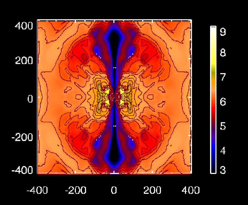
Figure 12.— Same with Fig.11(b), but for a wider region.

4.1. Method of Calculation

We have done a 2D GRMHD simulation of a collapsar using the Modified Kerr-Schild coordinate and $G=c=M=1$ units. When we show results, the coordinate is transfered from the Modified Kerr-Schild coordinate to the Kerr-Schild one, and the units are frequently transfered to cgs units. The calculated region corresponds to a quarter of the meridian plane under the assumption of axisymmetry and equatorial symmetry. The spherical mesh with 256($r$)$\times$ 128($\theta$) grid points is used for all the computations. The calculated region covers from $r=$1.8 to 3$\times 10^{4}$ (that corresponds to 5.3$\times 10^{5}$cm and 8.9$\times 10^{9}$cm in cgs units, as explained below) with uniform grids in the Modified Kerr-Schild space.

We adopt the model 12TJ in Woosley and Heger (2006). This model corresponds to a star that has 12$M_{\odot}$ initially with 1$\%$ of solar metallicity, and rotates rapidly and does not lose its angular momentum so much by adopting small mass loss rate. As a result, this star has a relatively large iron core of $1.82M_{\odot}$, and rotates rapidly (the estimated Kerr parameter that a BH forming of mass and angular momentum of the inner 3 $M_{\odot}$ would formally have is 0.57) at the final stage. Of course, what kind of stars are appropriate for progenitors of GRBs is still under debate Yoon et al. (2006). Thus we chosed the model 12TJ as a first example of our study because the iron core is large and rotating rapidly, which seems to form a rapidly-rotating BH, among the models listed in Woosley and Heger (2006). We assume that the central part of the star with 2$M_{\odot}$ has collapsed and formed a BH at the center with the Kerr parameter $a=0.5$. We also assume that the gravitational mass of the BH is unchanged throughout the calculation. Since $M=2M_{\odot}$, $r=1$ corresponds to 2.95 $\times 10^{5}$cm, as explained above. Also, the inner boundary $r=1.8$ is set within the outer horizon $r_{+}=1+\sqrt{1-a^{2}}=1.866$.

Since 1-D calculation is done for the model 12TJ, we can use the data directly only for the physical quanta on the equatorial plane. As for the density, internal energy density, and radial velocity, we assume the structure of the star is spherically symmetric. We also set $u^{\theta}=0$ initially. As for $u^{\phi}$, we extrapolate its value such as $u^{\phi}(r,\theta)=u^{\phi}(r,\pi/2)\times\sin\theta$.

Effects of magnetic fields are taken into account in the model 12TJ. However, again, since 1-D calculation is done, we do not know the configuration of the magnetic fields. It is difficult to extrapolate magnetic fields that satisfy the condition div$\bf B$ = 0 everywhere. Also, there are much uncertainty on the amplitude of the magnetic fields in a progenitor. Thus we do not use the information on magnetic fields of the model 12TJ. Rather, we adopt the same treatment in section 3.6. That is, the vector potential $A_{\phi}\propto{\rm max}(\rho/\rho_{\rm max}-0.2,0)\sin^{4}\theta$ where $\rho_{\rm max}$ is the peak density in the progenitor (after extracting the central part of the progenitor that has collapsed and formed a BH). The field is normalized so that the minimum value of $p_{\rm gas}/p_{\rm mag}$ becomes $10^{2}$. The definition of $p_{\rm mag}$ is $p_{\rm mag}=b^{2}/2$. The reason why we adopt the strong dependence on the zenith angle for $A_{\phi}$ is so as not to suffer from discontinuity of magnetic fields at the polar axis. The resulting biggest amplitude of the magnetic fields is 7.4$\times 10^{8}$G at $r=950$ (2.8$\times 10^{8}$cm).

We use a simple equation of state $p_{\rm gas}=(\gamma-1)u$ where we set $\gamma$=4/3 so that the equation of state roughly represents radiation gas.

As for the boundary condition in the radial direction, we adopt the outflow boundary condition for the inner and outer boundaries Gammie et al. (2003). As for the boundary condition in the zenith angle direction, axis of symmetry condition is adopted for the rotation axis, while the reflecting boundary condition is adopted for the equatorial plane. As for the magnetic fields, the equatorial symmetry boundary condition, in which the normal component is continuous and the tangential component is reflected, is adopted.

4.2. Results

In Fig.11, color contours of rest mass density at the central region are shown. Colors represent the density in units of g cm^-3 in logarithmic scale. These results are projected on the (r sin$\theta$,r cos $\theta$)-plane. The length $r=200$ corresponds to 5.9 $\times 10^{7}$ cm. The time unit corresponds to 9.85$\times 10^{-6}$ sec. Upper panel (a) represents the contours of rest mass density at $t=110000$ (that corresponds to 1.0835 sec), while lower panel shows the contours at $t=180000$ (that corresponds to 1.773 sec). Fig.12 is the same figure with Fig.11(b), but for a wider region. A jet is clearly seen along the rotation axis. In Fig.13, mass accretion rate history on the horizon is shown. The definition of the mass accretion rate is

$$\dot{M}=2\times 2\pi\int_{0}^{\theta}d\theta\sqrt{-g}\rho u^{r}.$$ (11)

It takes about 0.15 sec for the inner edge of the matter to reach the horizon. When the matter reaches there, there is an initial spike of the mass accretion rate. After that, there is a quasi-steady state like Fig.11(a) is realized. Then, the jet is launched at $\sim$1.1 sec. After that, the mass accretion rate varies rapidly with time, which resembles to a typical time profile of a GRB.

Figure 13.— Mass accretion rate history on the horizon. The unit $M_{\odot}$ sec^-1 is used assuming that the gravitational mass of the BH is 2$M_{\odot}$ throughout the calculation.

We show color contours of the plasma beta ($p_{\rm gas}/p_{\rm mag}$) in logarithmic scale at $t=180000$ in Fig.14. As expected, the plasma beta is low in the jet region while it is high in the accretion disk region. We show color contours of bulk Lorentz factor around the central region at $t=180000$ in Fig.15(a) (upper panel, in logarithmic scale). Color contours of the energy flux per unit rest-mass flux ($E=-T^{r}_{t}/(\rho u^{r})$), which is conserved for an inviscid fluid flow of magnetized plasma, are also shown in Fig.15(b) (lower panel, in logarithmic scale). This value represents the bulk Lorentz factor ($\Gamma_{\infty}$) of the invischid fluid element when all of the internal and magnetic energy are converted into kinetic energy at large distances McKinney 2006a . We can see that the bulk Lorentz factor of the jet is still low (Fig.15(a)), but it can be potentially as high as $10^{2}$ at large radius (Fig.15(b)). At $t=180000$, the strength of the magnetic field ($\sqrt{4\pi b^{2}}$) at the bottom of the jet is found to be $\sim 10^{15}$G, and $u^{\phi}$/$u^{t}$ is $\sim 0.1$ at $r_{\rm ms}$ on the equatorial plane. Here $r_{\rm ms}$ is the marginally stable orbit. For the Kerr BH with $a=0.5$, $r_{\rm ms}$ is 4.23. As stated in section 4.1, the initial biggest amplitude of the magnetic fields is 7.4$\times 10^{8}$G at $r=950$ where the initial density is $\sim 10^{6}$ g cm^-3, the expected amplification factor of the magnetic fields due to the gravitational collapse and differential rotation around the BH is $(\rho/\rho_{0})^{2/3}\times(d\Phi/dt/2\pi)*\Delta t$ $\sim$ 100 $\times$ 0.016 $\times$ 180000 $\sim 3\times 10^{5}$. Thus the initial magnetic field can be amplified as large as several times of $10^{14}$ G, which is roughly consistent with the amplitude of the magnetic fields at the bottom of the jet. At late phase, the magneto-rotational instability (MRI) may be also working, which is discussed in the next section.

In Fig.16, contours of the $\phi$ component of the vector potential ($A_{\phi}$) at $t=180000$ are shown. Level surfaces coincide with poloidal magnetic field lines, and field line density corresponds to poloidal field strength. As expected, the magnetic fields are strong at the jet region, which makes the plasma beta very low. From Fig.16, the opening angle of the jet is estimated as $5^{\circ}-6^{\circ}$. From Fig.14, 15(b), and 16, this jet should correspond to the poynting flux jet Hawley & Krolik (2006). This jet is surrounded by the funnel-wall jet region Hawley & Krolik (2006), which is shown in Fig.17 below.

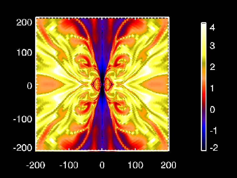
Figure 14.— Contour of the plasma beta ($p_{\rm gas}/p_{\rm mag}$) at $t=180000$ in logarithmic scale.

In Table.3 and 4, the integrated energies of matter and electromagnetic field at $t=180000$ are shown. The integrated region is between the horizon and $r=200$ (for Table.3) or $r=40$ (for Table.4), and within the zenith angle measured from the polar axis. As for the matter component, the contribution of the rest mass energy is subtracted. That is,

$$E_{\rm Matter}=2\times 2\pi\int_{r_{+}}^{r=200\;\rm or\;40}dr\int_{0}^{\theta}d\theta\sqrt{-g}(T^{0}_{0,\rm Matter}-\rho u^{0}u_{0}).$$ (12)

Factor 2 is coming from the symmetry of the system with respect to the equatorial plane. The field part can be written as

$$E_{\rm EM}=4\pi\int_{r_{+}}^{r=200\;\rm or\;40}dr\int_{0}^{\theta}d\theta\sqrt{-g}T^{0}_{0,\rm EM}.$$ (13)

It can be seen that the energy in electromagnetic field dominates that in matter within $r\leq 40$, while they become comparable within $r\leq 200$. Also, the integrated energy is still less than the typical explosion energy of a GRB ($\sim 5\times 10^{50}$erg; Frail et al. 2001).

Finally, we show the rest-mass density, outgoing mass flux, and outgoing poynting flux in Fig.17. The top panel (a) shows the rest-mass density (g cm^-3) as a function of the zenith angle at $r=10r_{\rm ms}=42.3$ and $t=180000$. It is seen that the low-density region is realized around the polar axis, which corresponds to the jet region (0.1 radian corresponds to 5.7^∘). The middle panel (b) shows the outgoing mass flux $\rho u^{r}$ (g cm^-2 s^-1) at $r=10r_{\rm ms}$ and $t=180000$. It is seen that the outgoing mass flux exists around $0.06\leq\theta\leq 0.14$, which corresponds to the funnel-wall jet (De Villiers et al., 2003; Hirose et al., 2004; McKinney & Gammie, 2004; Kato et al., 2004; De Villiers et al., 2005; Hawley & Krolik, 2006). The bottom panel (c) shows the outgoing poynting flux (in units of 10⁵⁰erg s^-1 rad^-1) at $r=r_{+}$ and $t=180000$. Definition of the outgoing poynting flux is

$$F_{\rm BZ}=-2\times 2\pi\sqrt{-g}T^{t}_{r,\rm EM}.$$ (14)

Factor 2 is coming from the assumption of the symmetry of the system with respect to the equatorial plane. We can see that the positive outgoing poynting flux exists at the jet region ($0\leq\theta\leq 0.23$ in radian). The integrated energy of the outgoing poynting flux at $r=r_{+}$ and $t=180000$ is $4.6\times 10^{46}$ erg s^-1. Since the duration of the jet in this study is $\sim 0.7$ s, this outgoing poynting flux seems to be too weak to explain the energy of the jet listed in Table.3 and 4. Thus we conclude that the jet is launched mainly by the magnetic field amplified by the gravitational collapse and differential rotation around the BH, rather than the Blandford-Znajek mechanism in this study.

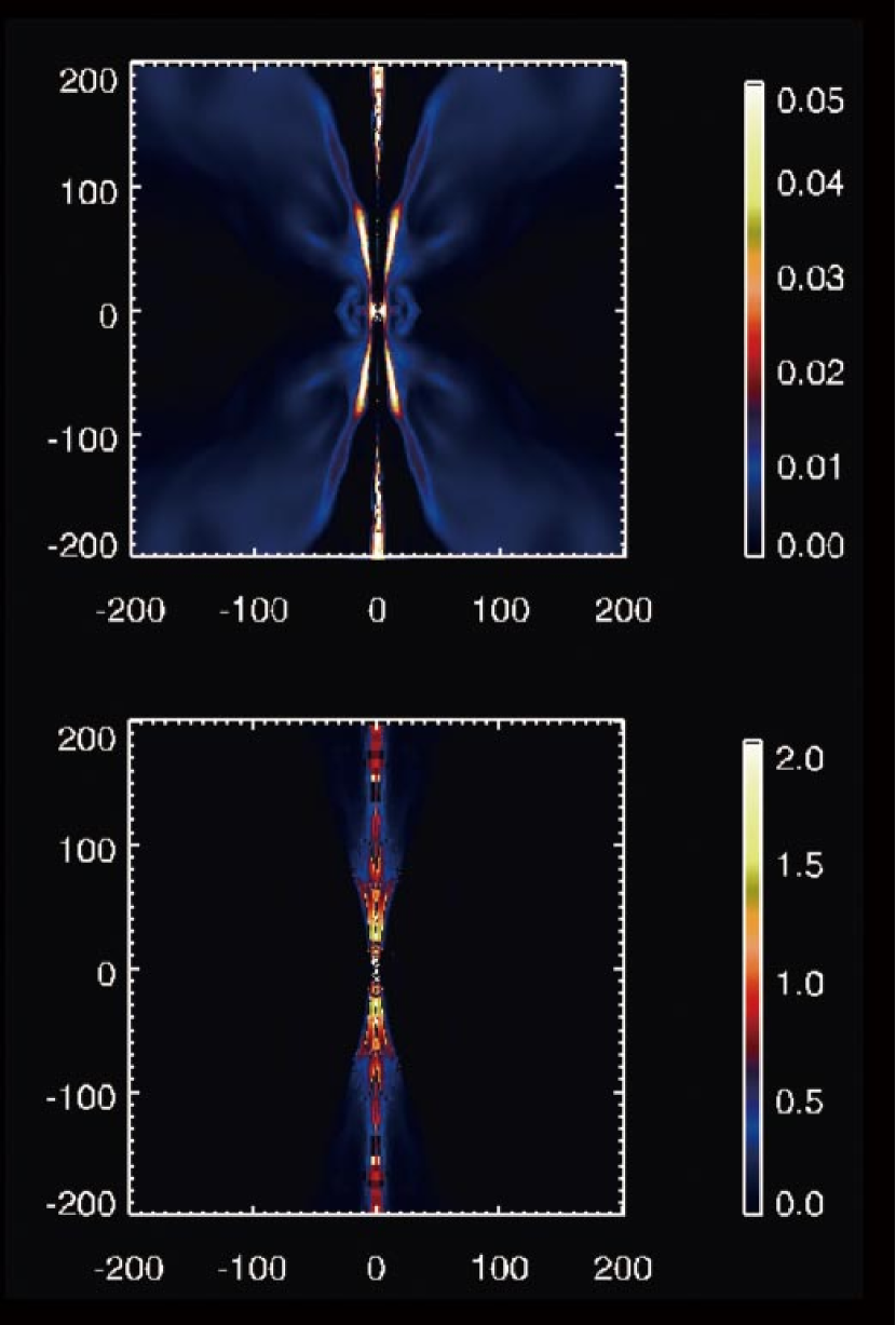
Figure 15.— Upper panel (a): contours of bulk Lorentz factor around the central region at $t=180000$. Lower panel (b): contours of the energy flux per unit rest-mass flux at $t=180000$ that represent the bulk Lorentz factor ($\Gamma_{\infty}$) of the invischid fluid element when all of the internal and magnetic energy are converted into kinetic energy at large distances. The contours are written in logarithmic scale.

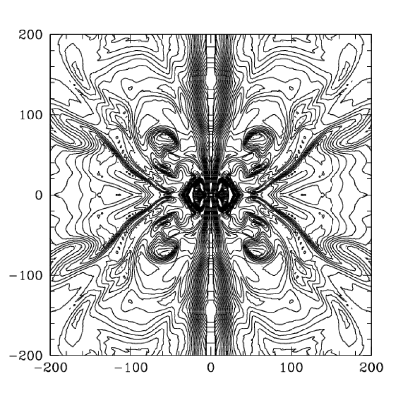
Figure 16.— Contours of the $\phi$ component of the vector potential ($A_{\phi}$) at $t=180000$. Level surfaces coincide with poloidal magnetic field lines, and field line density corresponds to poloidal field strength. The biggest amplitude of the magnetic fields is $\sim 10^{15}$G.

5. Summary and Discussion

In order to investigate the formation of relativistic jets at the center of a progenitor of a GRB, we have developed a two-dimensional GRMHD code. In order to confirm the reliability of the code, we have shown that the code passes many, well-known test calculations. Then we have performed a numerical simulation of a collapsar using a realistic progenitor model. We have followed the time evolution of the system for 1.773 s, and it was shown that a jet is launched from the center of the progenitor. We also found that the mass accretion rate is in quasi-stable state before the launch of the jet, while it shows rapid time variability that resembles to a typical time profile of a GRB after the launch. The structure of the jet is similar to the previous study: a poynting flux jet is surrounded by a funnel-wall jet. Even at the final stage of the simulation, the bulk Lorentz factor of the jet is still low, and the total energy of the jet is still as small as $10^{48}$ erg. However, we found that the energy flux per unit rest-mass flux ($E=-T^{r}_{t}/(\rho u^{r})$) is as high as $10^{2}$ at the at the bottom of the jet. Thus we conclude that the bulk Lorentz factor of the jet can be potentially high when it propagates outward. Also, as long as the duration of the activity of the central engine is long enough, the total energy of the jet can be large enough to explain the typical explosion energy of a GRB ($\sim 5\times 10^{50}$ erg). It is shown that the outgoing poynting flux exists at the horizon around the polar region, which proves that the Blandford-Znajek mechanism is working. However, we conclude that the jet is launched mainly by the magnetic field amplified by the gravitational collapse and differential rotation around the BH, rather than the Blandford-Znajek mechanism in this study.

When we apply the Blandford-Znajek formula Barkov & Komissarov 2008b , the integrated outgoing poynting flux is

$$\dot{E}=3.6\times 10^{50}f(a)\Psi^{2}_{27}M_{2}^{-2}\;\;\rm erg\;s^{-1}$$ (15)

where $M_{2}=M_{\rm BH}/2M_{\odot}=1$, $\Psi_{27}=\Psi/10^{27}$ G cm², and $f(a)=a^{2}/(1+\sqrt{1-a^{2}})^{2}=0.07179$. This value becomes $2.3\times 10^{46}B_{15}^{2}$ erg s^-1 for the jet with opening angle $\theta=5^{\circ}$, which is comparable to our numerical result (Fig.17(c)).

Figure 17.— The top panel (a): the rest-mass density (g cm^-3) as a function of the zenith angle at $r=10r_{\rm ms}=42.3$. The middle panel (b): the outgoing mass flux $\rho u^{r}$ (g cm^-2 s^-1) at $r=10r_{\rm ms}$. The bottom panel (c): the outgoing poynting flux (in units of 10⁵⁰erg s^-1 rad^-1) at $r=r_{+}$. These values are evaluated at the final stage of the simulation ($t=180000$).

As for the efficiency of converting the released gravitational energy to the jet’s energy, it can be estimated as follows: the mass accretion rate is $\sim 0.1M_{\odot}$ s^-1 (Fig.13), the total energy of the jet at the final stage is $\sim 10^{48}$ erg (Table.3), and the duration of the jet is $\sim 0.7$ s (Fig.13). Thus the efficiency can be estimated as $\sim 10^{-5}$. When we use the outgoing poynting flux at the horizon (4.6$\times 10^{46}$erg s^-1), the efficiency is as low as $\sim 3\times 10^{-7}$. These values seem to be very small compared with the previous study (De Villiers et al., 2005; Mckinney & Narayan 2007a, ). One of the reason will be because they used an almost steady disk model. On the other hand, we used a realistic progenitor model that collapses gravitationally. Thus the resulting mass accretion rate is pretty high. Second reason may be because the efficiency is still low even at the final stage of the simulation. If we perform the simulation further, the efficiency may become higher with time: mass accretion rate will become smaller, and the jet energy might be larger due to the amplification of the magnetic fields due to winding-up (and MRI) effects. Also, when the initial amplitude of the magnetic field is set to be larger (as in Barkov and Komissarov 2008), the efficiency may be enhanced. Further, we should investigate the dependence of the dynamics on progenitor models as well as the Kerr parameter of the BH. We are planning to investigate this point systematically in the next paper.

It is well known that the system is unstable against MRI when there is a strong negative shear profile $(d\Omega/d\ln r)$ (Balbus & Hawley, 1991, 1994), where $\Omega$ is the angular velocity. The saturation toroidal magnetic field strength is roughly expected to be $B_{\phi}\sim(4\pi\rho)^{1/2}r\Omega$ (Akiyama et al., 2003; Akiyama & Wheeler, 2005), which is confirmed by semi-global simulations Obergaulinger et al. (2008). The saturation poloidal magnetic field strength is roughly an order of magnitude smaller Obergaulinger et al. (2006). Thus $B_{\phi}$ may be amplified by MRI as strong as $1.4\times 10^{15}$G $\rho_{9}r_{\rm ms}\Omega_{4}$ where $\Omega_{4}$ is $\Omega/10^{4}$ rad s^-1. The characteristic timescale for saturating the MRI is the Alfv$\rm\acute{e}$n crossing time: $t_{A}\sim 0.1$ms $R_{6}\rho_{9}^{1/2}B_{15}^{-1}$ where $R_{6}$, $\rho_{9}$, and $B_{15}$ are the radius in units of $10^{6}$cm, the density in units of $10^{9}$ g cm^-3, and the amplitude of magnetic fields in units of $10^{15}$G, respectively. Thus this characteristic timescale can be shorter than the winding-up timescale for strong magnetic fields. However, the length scale of the mode with the largest MRI growth rate is approximately $\lambda_{\rm MRI}\sim 50$ cm $P_{0.5}B_{10}\rho_{9}^{-1/2}$ where $P_{0.5}$ is the rotation period in units of 0.5 ms, which is too short to be resolved numerically. At least, it is not resolved in the beginning of the simulations. After the magnetic field is amplified to a certain value due to gravitational collapse and winding-up effect, MRI may be working in this study (Obergaulinger et al. 2006b, ; Ott et al., 2006; Burrows et al., 2007; Dessart et al., 2008). It will be necessary to develop a sophisticated code that takes into account the MRI effectively with help of semi-global simulations Obergaulinger et al. (2008) in order to evaluate the influence of MRI on the dynamics of a collapsar.

It is well known that it becomes difficult to obtain the matter part of the primitive variables ($\rho$,$u$,$u^{i}$) precisely by the Newton-Raphson method Noble et al. (2006) due to numerical truncation errors (Komissarov, 2002; Komissarov 2004a, ; Komissarov 2004b, ; McKinney & Gammie, 2004; Komissarov, 2005; Mckinney 2006b, ) when the electromagnetic part of the stress energy tensor ( $T^{\mu\nu}_{\rm EM}$) greatly exceeds the matter part ( $T^{\mu\nu}_{\rm Matter}$). The problem is that the time integration of the electromagnetic part does not become so reliable, either. This is because the MHD condition ($u_{\mu}F^{\mu\nu}=0$) is implicitly assumed in the basic equations, and the resulting basic equation of electromagnetic part depends on the velocity of fluid (Eq.3). Such pathological conditions may be realized at the bottom of the jet in our study. In order to confirm the validity of our results in this study, we are planning to develop a general relativistic force-free code that is coupled with the GRMHD code sophisticatedly Mckinney 2006b .

It is very important to evaluate the terminal bulk Lorentz factor, because GRBs are considered to be emissions from relativistic flows with their bulk Lorentz factors greater than $10^{2}$ (e.g. Lithwick & Sari (2001)). Although an ad-hoc thermal (and kinetic) energy deposition into the polar region seems to lead to relativistic jets with bulk Lorentz factors $\sim 100$ (Aloy et al., 2000, 2002; Zhang et al., 2003, 2004; Cannizzo et al., 2004; Mizuta et al., 2006; Mizuta & Aloy, 2008; Morsony et al., 2007; Wang et al., 2008), it is still controversial whether such ad-hoc energy deposition is justified by numerical simulations with proper neutrino physics Nagataki et al. (2007). On the other hand, numerical study on the acceleration of electromagnetically powered jet requires quite high-resolution (Komissarov et al., 2007; Narayan et al., 2007; Tchekhovskoy et al., 2008; Komissarov et al., 2008). Due to the reason, a simplified jet model with an idealized boundary condition is used at present in order to investigate whether the initial poynting flux can be effectively converted into kinetic energy (Tchekhovskoy et al., 2008; Komissarov et al., 2008). According to their results, as long as confinement of the jet is realized, acceleration operates over several decades in radius and considerable fraction of the poynting flux can be converted into the kinetic energy. Thus, from the high-ratio of the poynting flux relative to rest-mass flux seen in our study (Fig.15(b)), a relativistic jet with high bulk Lorentz factor may be realized at large radius.

It is true that the two-dimensional restriction can be a significant limitation. First, anti-dynamo theorem Moffat (1978) prevents the indefinite maintenance of the poloidal magnetic field in the face of dissipation. Second, axisymmetric simulations tend to overemphasize the channel mode Hawley & Balbus (1992), which produces coherent internal magnetized flows rather than the more generic MHD turbulence. Hydrodynamic instability in the azimuthal direction may be also very important (Nagakura & Yamada, 2008, 2009). Thus we are planning to develop a three-dimensional GRMHD code (De Villiers et al., 2003; Hirose et al., 2004; De Villiers et al., 2005; Hawley & Krolik, 2006; Beckwith et al., 2008; Shafee et al., 2008; Mckinney & Blandford, 2008) and investigate the difference between two-dimensional simulations of collapsars with three-dimensional ones.

In this study, we assumed that the central region of the progenitor has collapsed and a BH is formed at the center with surrounding envelope unchanged. Thus we solved the GRMHD equation on a fixed background. But the final goal of our project is to study how a GRB is formed from the gravitational collapse of a massive star. Thus we are planning to develop a GRMHD code on a dynamical background, which makes the study on the gravitational collapse and BH formation at the center of a massive star possible (Shibata, 2003; Sekiguchi & Shibata, 2004, 2005; Baiotti et al., 2005; Duez et al., 2006; Sekiguchi & Shibata, 2007).

In this study, photo-disintegration of nuclei and neutrino processes are not taken into account. Photo-disintegration absorb considerable amount of thermal energy, and cooling/heating due to neutrino processes may have great influence on the dynamics of a collapsar (Di Matteo et al., 2002; Kohri & Mineshige, 2002; Nagataki et al. 2003a, ; Surman & McLaughlin, 2004; Lee et al., 2005; Gu et al., 2006; Nagataki et al., 2007; Kawanaka & Mineshige, 2007; Kawabata et al., 2008; Rossi et al., 2008; Zhang & Dai, 2009; Cannizzo & Gehrels, 2009). Especially, pair-annihilation of electron-type neutrinos may be a key process to drive a GRB jet (Woosley, 1993; MacFadyen & Woosley, 1999; Asano & Fukuyama, 2000, 2001; Miller et al., 2003; Surman & McLaughlin, 2005; Kneller et al., 2006; Shibata et al., 2007; Birkl et al., 2007). Thus we are planning to include such microphysics in our code, and perform more realistic simulations of collapsars.

The SNe associated with GRBs often show peculiar properties. Some are very energetic and blight (Galama et al., 1998; Iwamoto et al., 1998; Hjorth et al., 2003; Malesani et al., 2004), but others prohibit such blight SNe from being accompanied (Fynbo et al., 2006; Della Valle et al., 2006; Gal-Yam et al., 2006). Since the brightness of SNe depends on the mass of produced $\rm{}^{56}Ni$ (Woosley et al., 1999; Nakamura et al., 2001), it is suggested that there is a huge variety of the amount of $\rm{}^{56}Ni$ in a SN that associates with a GRB. It is still controversial where and when $\rm{}^{56}Ni$ is produced in a SN accompanied by a GRB (Nagataki et al. 2003b, ; Nagataki et al., 2006). It may be produced in a GRB jet (Maeda et al., 2002; Maeda & Nomoto, 2003; Tanaka et al., 2007; Maeda et al., 2008; Tominaga, 2009; Maeda & Tominaga, 2009; Bucciantini et al., 2009), or it may be produced in (or outflow from) the accretion disk around the BH (MacFadyen & Woosley, 1999; Pruet et al., 2004; Fujimoto et al., 2004; Surman et al., 2006; Hu & Peng, 2008), or it may be synthesized around a proto-neutron star Uzdensky & MacFadyen (2007). At present, it is impossible to investigate the explosive nucleosynthesis in a collapsar in our code because nuclear reactions are not taken into account. We are planning to include this effect, and study the site of $\rm{}^{56}Ni$ production. Also, study of a GRB as a possible site where very heavy elements and light elements are synthesized is very important (Lemoine, 2002; Beloborodov, 2003; Suzuki & Nagataki, 2005).

Table 1Initial Conditions for Shock Tube Test1 and Collision Test

Test Type		$\rho$	$p$	$v^{x}$	$v^{y}$	$v^{z}$	$B^{x}$	$B^{y}$	$B^{z}$
Shock Tube Test1	left state	1	1000	0	0	0	1	0	0
	right state	0.1	1	0	0	0	1	0	0
Collision Test	left state	1	1	5/$\sqrt{26}$	0	0	10	10	0
	right state	1	1	-5/$\sqrt{26}$	0	0	10	-10	0

Table 2Initial Conditions for 2D Shock Tube Problem

Region	$x$	$y$	$\rho$	$p$	$v^{x}$	$v^{y}$
A	0 $\leqq$ $x$ $\leqq$ 0.5	0.5 $\leqq$ $y$ $\leqq$ 1	0.1	1	0.99	0
B	0.5 $\leqq$ $x$ $\leqq$ 1	0.5 $\leqq$ $y$ $\leqq$ 1	0.1	0.01	0	0
C	0 $\leqq$ $x$ $\leqq$ 0.5	0 $\leqq$ $y$ $\leqq$ 0.5	0.5	1	0	0
D	0.5 $\leqq$ $x$ $\leqq$ 1	0 $\leqq$ $y$ $\leqq$ 0.5	0.1	1	0	0.99

Table 3Integrated Energies of Matter and Field (r$\leq$200)

$\theta$	$0.714^{\circ}$	$1.43^{\circ}$	$2.14^{\circ}$	$2.86^{\circ}$	$3.57^{\circ}$
Matter	1.44E+46	7.09E+46	1.70E+47	3.14E+47	5.10E+47
Field	2.96E+46	1.11E+47	2.39E+47	4.12E+47	6.30E+47
$\theta$	$4.29^{\circ}$	$5.00^{\circ}$	$5.71^{\circ}$	$6.42^{\circ}$	$7.14^{\circ}$
Matter	7.66E+47	1.10E+48	1.52E+48	2.05E+48	2.69E+48
Field	8.91E+47	1.19E+48	1.52E+48	1.88E+48	2.26E+48

Table 4Integrated Energies of Matter and Field (r$\leq$40)

$\theta$	$0.714^{\circ}$	$1.43^{\circ}$	$2.14^{\circ}$	$2.86^{\circ}$	$3.57^{\circ}$
Matter	6.89E+43	3.15E+44	8.96E+44	2.03E+45	3.95E+45
Field	8.60E+45	3.44E+46	7.73E+46	1.37E+47	2.14E+47
$\theta$	$4.29^{\circ}$	$5.00^{\circ}$	$5.71^{\circ}$	$6.42^{\circ}$	$7.14^{\circ}$
Matter	6.76E+45	1.04E+46	1.47E+46	1.96E+46	2.50E+46
Field	3.08E+47	4.19E+47	5.46E+47	6.91E+47	8.52E+47

References

- Abramowicz et al. (1978) Abramowicz, M., Jaroszinski, M., Sikora, M. 1978, A&A, 63, 221
- Aloy et al. (2000) Aloy, M.A., Mller, E., Ibez, J.M., Mrt, J.M., MacFadyen, A. 2000, ApJ, 531, L119
- Aloy et al. (2002) Aloy, M.A., Ibez, J.M., Miralles, J.-A., Urpin, V. 2002, A&A, 396, 693
- Anninos et al. (2005) Anninos, P., Fragile, P.C., Salmonson, J.D. 2005, ApJ, 635, 723
- Antn et al. (2006) Antn, L., Zanotti, O., Miralles, J.A., et al. 2006, ApJ, 637, 296
- Akiyama et al. (2003) Akiyama, S., Wheeler, J.C., Meier, D.L., Lichtenstadt, I. 2003, ApJ, 584, 954
- Akiyama & Wheeler (2005) Akiyama, S., Wheeler, J.C. 2005, ApJ, 629, 414
- Asano & Fukuyama (2000) Asano, K., Fukuyama, T. 2000, ApJ, 531, 949
- Asano & Fukuyama (2001) Asano, K., Fukuyama, T. 2001, ApJ, 546, 1019
- Baiotti et al. (2005) Baiotti, L. et al. 2005, Phys. Rev. D, 71, 024035
- Balbus & Hawley (1991) Balbus, S.A., Hawley, J.F. 1991, ApJ, 376, 214
- Balbus & Hawley (1994) Balbus, S.A., Hawley, J.F. 1994, MNRAS, 266, 769
- Balsara (2001) Balsara, D. 2001, ApJS, 132, 83
- (14) Barkov, M., Komissarov, S.S. 2008, MNRAS, 385, L28
- (15) Barkov, M., Komissarov, S.S. 2008, arXiv:0809.1402
- Beckwith et al. (2008) Beckwith, K., Hawley, J.F., Krolik, J.H. 2008, ApJ, 678, 1180
- Beloborodov (2003) Beloborodov, A.M. 2003, ApJ, 588, 931
- Bethe (1990) Bethe, H.A. 1990, Rev. Mod. Phys., 62, 801
- Birkl et al. (2007) Birkl, R., Aloy, M.A., Janka, H.-Th., Mller, E. 2007, A&A, 463, 51
- Blandford & Znajek (1977) Blandford, R.D., Znajek, R.L. 1977, MNRAS, 179, 433
- Blandford & Payne (1982) Blandford, R.D., Payne, D.G. 1982, MNRAS, 199, 883
- Bucciantini et al. (2008) Bucciantini, N., Quataert, E., Arons, J., Metzger, B.D., Thompson, T.A. 2008, MNRAS, 383, 25
- Bucciantini et al. (2009) Bucciantini, N., Quataert, E., Metzger, B.D., Thompson, T.A., Arons, J., Del Zanna, L. 2009, arXiv:0901.3801
- Burrows et al. (2007) Burrows, A., Dessart, L., Livne, E., Ott, C.D., Murphy, J. ApJ, 664, 416
- Cannizzo et al. (2004) Cannizzo, J.K., Gehrels, N., Vishniac, E.T. 2004, ApJ, 601, 380
- Cannizzo & Gehrels (2009) Cannizzo, J.K., Gehrels, N. 2009, arXiv:0901.3564
- De Villiers & Hawley (2003) De Villiers, J.-P., Hawley, J.F. 2003, ApJ, 589, 458
- De Villiers et al. (2003) De Villiers, J.-P., Hawley, J.F., Krolik, J.H. 2003, ApJ, 599, 1238
- De Villiers et al. (2005) De Villiers, J.-P., Hawley, J.F., Krolik, J.H., Hirose, S. 2005, ApJ, 620, 878
- Del Zanna & Bucciantini (2001) Del Zanna, L., Bucciantini, N. 2002, A&A, 390, 1177
- Del Zanna et al. (2003) Del Zanna, L., Bucciantini, N., Londrillo, P. 2003, A&A, 400, 397
- Del Zanna et al. (2007) Del Zanna, L., Zanotti, O., Bucciantini, N., Londrillo, P. 2007, A&A, 473, 11
- Della Valle et al. (2006) Della Valle, M., et al. 2006, Nature, 444, 1050
- Dessart et al. (2008) Dessart, L., Burrows, A., Livne, E., Ott, C.D. 2008, ApJ, 673, L43
- Di Matteo et al. (2002) Di Matteo, T., Perna, R., Narayan, R. 2002, ApJ, 579, 706
- Duez et al. (2006) Duez, M.D., Liu, Y.T., Shapiro, S.L., Shibata, M., Stephens, B.C. 2006 Phys. Rev. Lett., 96, 031101
- Fishbone & Moncrief (1976) Fishbone, L.G., Moncrief, V. 1976, ApJ, 207, 962
- Frail et al. (2001) Frail, D.A., et al. 2001, ApJ, 562, L55
- Fryer & Mszros (2000) Fryer, C., Mszros, P. 2000, ApJ, 588, L25
- Fujimoto et al. (2004) Fujimoto, S., Hashimoto, M., Arai, K., Matsuba, R. 2004, ApJ, 614, 847
- Fujimoto et al. (2006) Fujimoto, S., et al. 2006, ApJ, 644, 1040
- Fynbo et al. (2006) Fynbo, J.P.U., et al. 2006, Nature, 444, 1047
- Galama et al. (1998) Galama, T.J., et al., 1998, Nature, 395, 670
- Gal-Yam et al. (2006) Gal-Yam, A., et al. 2006, Nature, 444, 1053
- Gammie (1999) Gammie, C.F. 1999, ApJ, 522, L57
- Gammie et al. (2003) Gammie, C.F., McKinney, J.C., Tth, G. 2003, ApJ, 589, 444
- Gu et al. (2006) Gu, W.-M., Liu, T., Lu, J.-F. 2006, ApJ, 643, L87
- Harten et al. (1983) Harten, A., Lax, P.D., van Lerr, B. 1983, SIAM Rev. 25, 35
- Hawley & Balbus (1992) Hawley, J.F., Balbus, S.A. 1992, ApJ, 400, 595
- Hawley & Krolik (2006) Hawley, J.F., Krolik, J.H. 2006, ApJ, 641, 103
- Hirose et al. (2004) Hirose, S., Krolik, J.H., De Villiers, J.-P., Hawley, J.F. 2004, ApJ, 606, 1083
- Hjorth et al. (2003) Hjorth, J., et al. 2003, Nature, 423, 847
- Hu & Peng (2008) Hu, T., Peng, Q. 2008, ApJ, 681, 96
- Iwamoto et al. (1998) Iwamoto, K., et al., 1998, Nature, 395, 672
- Kato et al. (2004) Kato, Y., Mineshige, S., Shibata, K. 2004, ApJ, 605, 307
- Kawabata et al. (2008) Kawabata, R., Mineshige, S., Kawanaka, N. 2008, ApJ, 675, 596
- Kawanaka & Mineshige (2007) Kawanaka, N., Mineshige, S. 2007, ApJ, 662, 1156
- Klebesadel et al. (1973) Klebesadel, R.W., Strong, I.B., Olson, R.A. 1973, ApJ, 182, L85
- Kneller et al. (2006) Kneller, J.P., McLaughlin, G.C., Surman, R.A. 2006, J. Phys. G., 32, 443
- Kohri & Mineshige (2002) Kohri, K., Mineshige, S. 2002, ApJ, 577, 311
- Komissarov (1999) Komissarov, S.S. 1999, MNRAS, 303, 343
- Komissarov (2002) Komissarov, S.S. 2002, MNRAS, 336, 759
- (63) Komissarov, S.S. 2004b, MNRAS, 350, 427
- (64) Komisarrov, S.S. 2004a, MNRAS, 350, 1431
- Komissarov (2005) Komissarov, S.S. 2005, MNRAS, 359, 801
- Komissarov et al. (2007) Komissarov, S.S., Barkov, M.V., Vlahakis, N., Knigl, A. 2007, MNRAS, 380, 51
- Komissarov & Barkov (2007) Komissarov, S.S., Barkov, M.V. 2007, MNRAS, 382, 1029
- Komissarov et al. (2008) Komissarov, S.S., Vlahakis, N., Knigl, A., Barkov, M.V. 2008, arXiv:0811.1467
- Lee et al. (2005) Lee, W.H., Rmirez-Ruiz, E., Page, D. 2005, ApJ, 632, 421
- Leismann et al. (2005) Leismann, T., Antn , L., Aloy, M.A., Mller, E., Mart, J.M., Miralles, J.A., Ibez, J.M. 2005, A&A, 436, 503
- Lemoine (2002) lemoine, M. 2002, A&A, 390, L31
- Lithwick & Sari (2001) Lithwick, Y., Sari, R. 2001, ApJ, 555, 540
- MacFadyen & Woosley (1999) MacFadyen, A.I., Woosley, S.E., ApJ, 1999, 524, 262
- Maeda et al. (2002) Maeda, K., et al., 2002, ApJ, 565, 405
- Maeda & Nomoto (2003) Maeda, K., Nomoto, K. 2003, ApJ, 598, 1163
- Maeda et al. (2008) Maeda, K., et al. 2008, Science, 319, 1220
- Maeda & Tominaga (2009) Maeda, K., Tominaga, N. 2009, arXiv:0901.0410
- Malesani et al. (2004) Malesani, D., et al. 2004, ApJ, 609, L5
- McKinney & Gammie (2004) McKinney, J.C., Gammie, C.F. 2004, ApJ, 611, 977
- (80) McKinney, J.C. 2006a, MNRAS, 368, 1561
- (81) McKinney, J.C. 2006b, MNRAS, 367, 1797
- (82) McKinney, J.C., Narayan, R. 2007a, MNRAS, 375, 513
- (83) McKinney, J.C., Narayan, R. 2007b, MNRAS, 375, 531
- Mckinney & Blandford (2008) McKinney, J.C., Blandford, R. 2008, arXiv:0812.1060
- Melesani et al. (2004) Melesani, D., et al. 2004, ApJ, 609, L5
- Miller et al. (2003) Miller, W., George, N.D., Kheyfets, A., McGhee, J.M. 2003, ApJ, 583, 833
- Misner et al. (1970) Misner, J.C., Thorne, K., Wheeler, J.A., Gravitation (W.H. Freeman and Co., San Francisco, 1970)
- (88) Mizuno, Y., Yamada, S., Koide, S., Shibata, K. 2004a, ApJ, 606, 395
- (89) Mizuno, Y., Yamada, S., Koide, S., Shibata, K. 2004b, ApJ, 615, 389
- Mizuno et al. (2006) Mizuno, Y., Nishikawa, K., Koide, S., Hardee, P., Fishman, G.J. 2006, astro-ph/0609004
- Mizuta et al. (2006) Mizuta, A., Yamasaki, T., Nagataki, S., Mineshige, S. 2006, ApJ, 651, 960
- Mizuta & Aloy (2008) Mizuta, A., Aloy, M.A. 2008, arXiv:0812.4813
- Moffat (1978) Moffat, K. 1978, Magnetic Field Generation in electrically Conducting Fluids (Cambridge: Cambridge Univ. Press)
- Morsony et al. (2007) Morsony, B.J., Lazzati, D., Begelman, M.C. 2007, ApJ, 665, 569
- Nagakura & Yamada (2008) Nagakura, H., Yamada, S. 2008, ApJ, 689, 391
- Nagakura & Yamada (2009) Nagakura, H., Yamada, S. 2009, arXiv:0901.4053
- (97) Nagataki, S., Kohri, K., Ando, S., Sato, K. 2003a, APh, 18, 551
- (98) Nagataki, S., Mizuta, A., Yamada, S. Takabe, H., Sato, K. 2003b, ApJ, 596, 401
- Nagataki et al. (2006) Nagataki, S., Mizuta, A., Sato, K. 2006, ApJ, 647, 1255
- Nagataki et al. (2007) Nagataki, S., Takahashi, R., Mizuta, A., Takiwaki, T. 2007, ApJ, 659, 512
- Nakamura et al. (2001) Nakamura, T., et al. 2001, ApJ, 555, 880
- Narayan et al. (2007) Narayan. R., McKinney, J.C., Farmer, A.J. 2007, MNRAS, 375, 548
- Noble et al. (2006) Noble, S.C., Gammie, C.F., McKinney, J.C., Del Zanna, L. 2006, ApJ, 641, 626
- Obergaulinger et al. (2006) Obergaulinger, M., Aloy, M.A., Mller, E. 2006, A&A, 450, 1107
- (105) Obergaulinger, M., Aloy, M.A., Dimmelmeier, H., Mller, E. 2006, A&A, 457, 209
- Obergaulinger et al. (2008) Obergaulinger, M., Cerd-Durn, P., Mller, E., Aloy, M.A. 2008, arXiv:0811.1652
- Ott et al. (2006) Ott, C.D., Burrows, A., Thompson, T.A., Livne, E., Walder, R. 2006, ApJS, 164, 130
- Proga et al. (2003) Proga, D., MacFadyen, A.I., Armitage, P.J., Begelman, M.C. 2003, ApJ, 599, L5
- Proga & Begelman (2003) Proga, D., Begelman, M.C. 2003, ApJ, 582, 69
- Proga (2005) Proga, D. 2005, ApJ, 629, 397
- Pruet et al. (2004) Pruet, J., Thompson, T.A., Hoffman, R.D. 2004, ApJ, 606, 1006
- Rossi et al. (2008) Rossi, E.M., Armitage, P.J., Menou, K. 2008, MNRAS, 391, 922
- Sekiguchi & Shibata (2004) Skiguchi, Y., Shibata, M. 2004, Phys. Rev. D, 70, 084005
- Sekiguchi & Shibata (2005) Skiguchi, Y., Shibata, M. 2005, Phys. Rev. D, 71, 084013
- Sekiguchi & Shibata (2007) Skiguchi, Y., Shibata, M. 2007, PThPh, 117, 1029
- Shafee et al. (2008) Shafee, R., et al. 2008, ApJ, 687, L25
- Shibata (2003) Shibata, M. 2003, Phys. Rev. D, 67, 024033
- Shibata et al. (2006) Shibata, M., Liu, Y.T., Shapiro, S.L., Stephens, B.C. 2006, Phys. Rev. D, 74, 104026
- Shibata et al. (2007) Shibata, M., Sekiguchi, Y., Takahashi, R. 2007, PThPh, 118, 257
- Surman & McLaughlin (2004) Surman, R., McLaughlin, G.C. 2004, ApJ, 603, 611
- Surman & McLaughlin (2005) Surman, R., McLaughlin, G.C. 2005, ApJ, 618, 397
- Surman et al. (2006) Surman, R., McLaughlin, G.C., Hix, W.R. 2006, ApJ, 643, 1057
- Suwa et al. (2007) Suwa, Y., Takiwaki, T., Kotake, K., Sato, K. 2007, PASJ, 59, 771
- Suzuki & Nagataki (2005) Suzuki, T.K., Nagataki, S. 2005, ApJ, 628, 914
- Takahashi et al. (1990) Takahashi, M., Nitta, S., Tatematsu, Y., Tomimatsu, A. 1990, ApJ, 363, 206
- Takiwaki et al. (2004) Takiwaki, T., Kotake, K., Nagataki, S., Sato, K. 2004, ApJ, 616, 1086
- Takiwaki et al. (2008) Takiwaki, T., Kotake, K., Sato, K. 2008, arXiv:0712.1949
- Tanabe & Nagataki (2008) Tanabe, K., Nagataki, S. 2008, Phys. Rev. D, 78, 024004
- Tanaka et al. (2007) Tanaka, M., Maeda, K., Mazzali, P.A., Nomoto, K. 2007, ApJ, 668, L19
- Tchekhovskoy et al. (2007) Tchekhovskoy, A., McKinney, J.C., Narayan, R. 2007, MNRAS, 379, 469
- Tchekhovskoy et al. (2008) Tchekhovskoy, A., McKinney, J.C., Narayan, R. 2008, MNRAS, 388, 511
- Tominaga (2009) Tominaga, N. 2009, ApJ, 690, 526
- Tth (2000) Tth, J. 2000, Compt. Phys. 161, 605
- Usov (1992) Usov, V.V. 1992, Nature, 357, 472
- Uzdensky & MacFadyen (2007) Uzdensky, D.A., MacFadyen, A.I. 2007, ApJ, 669, 546
- van Leer (1977) van Leer, B.J. 1977, J. Compt. Phys. 23, 276
- Yoon et al. (2006) Yoon, S.-C., Langer, N., Norman, C. 2006, A&A, 460, 199
- Wang et al. (2008) Wang, P., Abel, T., Zhang, W. 2008, ApJ, 176, 467
- Woosley (1993) Woosley, S.E., ApJ, 1993, 405, 273
- Woosley et al. (1999) Woosley, S.E., Eastman, R.G., Schmidt, B.P. 1999, ApJ, 516, 788
- Woosley & Bloom (2006) Woosley, S.E., Bloom, J. 2006, ARA&A, 44, 507
- Woosley & Heger (2006) Woosley, S.E., Heger, A. 2006, ApJ, 637, 914
- Zhang & Dai (2009) Zhang, D., Dai, Z.G. 2009, arXiv:0901.0431
- Zhang et al. (2003) Zhang, W., Woosley, S.E., MacFadyen, A. 2003, ApJ, 586, 356
- Zhang et al. (2004) Zhang, W., Woosley, S.E., Heger, A. 2003, ApJ, 608, 365
- Zhang & MacFadyen (2006) Zhang, W., MacFadyen, A.I. 2006, ApJS, 164, 255