Alternative quantization of the Hamiltonian in isotropic loop quantum cosmology

Abstract

Since there are quantization ambiguities in constructing the Hamiltonian constraint operator in isotropic loop quantum cosmology, it is crucial to check whether the key features of loop quantum cosmology, such as the quantum bounce and effective scenario, are robust against the ambiguities. In this paper, we consider a typical quantization ambiguity arising from the quantization of the field strength of the gravitational connection. An alternative Hamiltonian constraint operator is constructed, which is shown to have the correct classical limit by the semiclassical analysis. The effective Hamiltonian incorporating higher order quantum corrections is also obtained. In the spatially flat FRW model with a massless scalar field, the classical big bang is again replaced by a quantum bounce. Moreover, there are still great possibilities for the expanding universe to recollapse due to the quantum gravity effect. Thus, these key features are robust against this quantization ambiguity.

I Introduction

An important motivation of the theoretical search for a quantum theory of gravity is the expectation that the singularities predicted by classical general relativity would be resolved by the quantum gravity theory. This expectation has been confirmed by the recent study of certain isotropic models in loop quantum cosmology (LQC) bojowald ; apsL ; aps , which is a simplified symmetry-reduced model of a full background-independent quantum theory of gravity lrr , known as loop quantum gravity (LQG) rev ; rov ; thie ; hhm . In loop quantum cosmological scenario for a universe filled with a massless scalar field, the classical singularity gets replaced by a quantum bounce aps ; bojow-r ; AshR . Moreover, it is revealed in the effective scenarios that there are great possibilities for a spatially flat FRW expanding universe to recollapse due to the quantum gravity effect dmy . However, as in the ordinary quantization procedure, there are quantization ambiguities in constructing the Hamiltonian constraint operator. Thus a crucial question arises. Whether the above significant results come from certain particular treatment of quantization? Before confirming the robustness of the key results against the quantization ambiguities, one could not believe that they are not some artifact under particular assumptions.

In this paper, we consider a typical quantization ambiguity arising from the quantization of the field strength of the gravitational connection. An alternative Hamiltonian constraint operator is constructed. Semiclassical states are then employed to show that the new Hamiltonian operator has the correct classical limit. The effective Hamiltonian incorporating higher order quantum corrections is also obtained. In the spatially flat FRW model with a massless scalar field, the classical big bang is again replaced by a quantum bounce. Moreover, there are still great possibilities for the expanding universe to recollapse due to the quantum gravity effect.

In the spatially flat isotropic model of LQC, one has to first introduce an elementary cell ${\cal V}$ and restrict all integrations to this cell. Fix a fiducial flat metric ${{}^{o}\!q}_{ab}$ and denote by $V_{o}$ the volume of the elementary cell ${\cal V}$ in this geometry. The gravitational phase space variables —the connections $A_{a}^{i}$ and the density-weighted triads $E^{a}_{i}$— can be expressed as

$$A_{a}^{i}=c\,V_{o}^{-1/3}\,\,{}^{o}\!\omega_{a}^{i}\quad\mathrm{and}\quad E^{a}_{i}=p\,V_{o}^{-2/3}\,\sqrt{{}^{o}\!q}\,\,{}^{o}\!e^{a}_{i},$$ (1)

where $({}^{o}\!\omega_{a}^{i},{}^{o}\!e^{a}_{i})$ are a set of orthonormal co-triads and triads compatible with ${{}^{o}\!q}_{ab}$ and adapted to the edges of the elementary cell ${\cal V}$. The basic (nonvanishing) Poisson bracket is given by

$$\{c,\,p\}=\frac{8\pi G\gamma}{3},$$ (2)

where $G$ is the Newton’s constant and $\gamma$ is the Barbero-Immirzi parameter.

To pass to the quantum theory, one constructs a kinematical Hilbert space ${\cal H}^{\mathrm{grav}}_{\mathrm{kin}}=L^{2}(\mathbb{R}_{\mathrm{Bohr}},{\mathrm{d}}\mu_{\mathrm{Bohr}})$, where $\mathbb{R}_{\mathrm{Bohr}}$ is the Bohr compactification of the real line and ${\mathrm{d}}\mu_{\mathrm{Bohr}}$ is the Haar measure on it math . The abstract $*$-algebra represented on the Hilbert space is based on the holonomies of connection $A^{i}_{a}$. In the Hamiltonian constraint of LQG, the gravitational connection $A^{i}_{a}$ appears through its curvature $F^{i}_{ab}$. Since there exists no operator corresponding to $c$, only holonomy operators are well defined. Hence one is led to express the curvature in terms of holonomies. Similarly, in the improved dynamics setting of LQC aps , to express the curvature one employed the holonomies

$$h_{i}^{(\bar{\mu})}:=\cos\frac{\bar{\mu}c}{2}\,\mathbb{I}+2\sin\frac{\bar{\mu}c}{2}\,\tau_{i}$$ (3)

along an edge parallel to the triad ${}^{o}\!e^{a}_{i}$ of length $\bar{\mu}\sqrt{|p|}$ with respect to the physical metric $q_{ab}$, where $\mathbb{I}$ is the identity $2\times 2$ matrix and $\tau_{i}=-i\sigma_{i}/2$ ($\sigma_{i}$ are the Pauli matrices). Thus, the elementary variables could be taken as the functions $\exp(i\bar{\mu}c/2)$ and the physical volume $V=|p|^{3/2}$ of the cell, which have unambiguous operator analogs.

II The alternative Hamiltonian constraint operator

In general relativity, the dynamics of a gravitational system is determined by the Hamiltonian constraint. Many problems, such as the big-bang singulary, arise in classical dynamics. One expects that some quantum dynamics can resolve these problems. Hence, it is important to have a well-defined Hamiltonian constraint operator in LQC. An improved Hamiltonian constraint operator has been constructed in aps . However, there are quantization ambiguities in the construction. In this section, we will construct an alternative Hamiltonian constraint operator by a different quantization procedure.

Because of spatial flatness and homogeneity, the gravitational part of the Hamiltonian constraint of full general relativity is simplified to the form

$$C_{\mathrm{grav}}=-\gamma^{-2}\int_{\cal V}{\mathrm{d}}^{3}xN\epsilon_{ijk}F^{i}_{ab}e^{-1}E^{aj}E^{bk},$$ (4)

where $e:=\sqrt{|\det{E}|}$, the lapse $N$ is constant and we will set it to one.

The procedure used in LQC (and specifically in aps ; math ) so far can be summarized as follows. The term involving the triads can be written as

$$\epsilon_{ijk}e^{-1}E^{aj}E^{bk} =\sum_{k}\frac{\mathrm{sgn}(p)}{2\pi\gamma G\bar{\mu}V_{o}^{1/3}}\,\,\epsilon^{abc}\,\,{}^{o}\!\omega_{c}^{k}$$

$$\quad\times\mathrm{Tr}\left(h_{k}^{(\bar{\mu})}\left\{{h_{k}^{(\bar{\mu})}}^{-1},V\right\}\tau_{i}\right).$$ (5)

To express the curvature components $F^{i}_{ab}$ in terms of holonomies, one considers a square $\Box_{ij}$ in the $i$-$j$ plane spanned by a face of ${\cal V}$, each of whose sides has length $\bar{\mu}\sqrt{|p|}$ with respect to $q_{ab}$. Then the $ab$ component of the curvature is given by

$$F^{i}_{ab}\tau_{i}=\lim_{Ar_{\Box}\rightarrow 0}\frac{h_{\Box_{ij}}^{(\bar{\mu})}-1}{\bar{\mu}^{2}V_{o}^{2/3}}{}^{o}\!\omega_{[a}^{i}{}^{o}\!\omega_{b]}^{j},$$ (6)

where $Ar_{\Box}$ is the area of the square under consideration, and the holonomy $h_{\Box_{ij}}^{(\bar{\mu})}$ around the square $\Box_{ij}$ is just the product of holonomies along the four edges of $\Box_{ij}$,

$$h_{\Box_{ij}}^{(\bar{\mu})}=h_{i}^{(\bar{\mu})}h_{j}^{(\bar{\mu})}{h_{i}^{(\bar{\mu})}}^{-1}{h_{j}^{(\bar{\mu})}}^{-1}.$$ (7)

However, quantization ambiguities arise here, since the approach to express the curvature components $F^{i}_{ab}$ in terms of holonomies is not unique. Hence the corresponding operators in different approaches will be different from each other. In the following, we will consider an expression of the curvature components different from Eq. (6). Taking account of the definition (3) of holonomies, we have the identity

$$\lim_{\bar{\mu}\rightarrow 0}\frac{h_{i}^{(\bar{\mu})}-{h_{i}^{(\bar{\mu})}}^{-1}}{\bar{\mu}}=\lim_{\bar{\mu}\rightarrow 0}\frac{4\sin(\bar{\mu}c/2)\,\tau_{i}}{\bar{\mu}}=2c\tau_{i}.$$ (8)

Hence the curvature of connection can be written in terms of the holomomies as

$$F^{k}_{ab}\tau_{k} =c^{2}V_{o}^{-2/3}\epsilon_{ijk}\,\,{}^{o}\!\omega_{a}^{i}\,\,{}^{o}\!\omega_{b}^{j}\tau_{k}$$

$$=\lim_{\bar{\mu}\rightarrow 0}\frac{\left(h_{i}^{(\bar{\mu})}-{h_{i}^{(\bar{\mu})}}^{-1}\right)\left(h_{j}^{(\bar{\mu})}-{h_{j}^{(\bar{\mu})}}^{-1}\right)}{2\bar{\mu}^{2}V_{o}^{2/3}}\,\,{}^{o}\!\omega_{[a}^{i}\,\,{}^{o}\!\omega_{b]}^{j}.$$ (9)

Combining Eqs. (II) and (II), the Hamiltonian constraint can be written as

$$C_{\mathrm{grav}} =-\lim_{\bar{\mu}\rightarrow 0}\frac{\mathrm{sgn}(p)}{4\pi\gamma^{3}G\bar{\mu}^{3}}\epsilon^{ijk}\mathrm{Tr}\Big{[}\left(h_{i}^{(\bar{\mu})}-{h_{i}^{(\bar{\mu})}}^{-1}\right)$$

$$\quad\quad\quad\quad\times\left(h_{j}^{(\bar{\mu})}-{h_{j}^{(\bar{\mu})}}^{-1}\right)h_{k}^{(\bar{\mu})}\left\{{h_{k}^{(\bar{\mu})}}^{-1},V\right\}\Big{]}$$

$$\equiv\lim_{\bar{\mu}\rightarrow 0}{C^{\mathrm{R}}}^{(\bar{\mu})}_{\mathrm{grav}}.$$ (10)

Since the constraint is now expressed in terms of elementary variables and their Poisson bracket, it can be promoted to a quantum operator directly. The resulting alternative regulated constraint operator with symmetric factor-ordering reads

$$\hat{C^{\mathrm{R}}}^{(\bar{\mu})}_{\mathrm{grav}} =\sin\frac{\bar{\mu}c}{2}\Big{[}\frac{12i\,\mathrm{sgn}(\hat{p})}{\pi\gamma^{3}\bar{\mu}^{3}\ell_{p}^{2}}\Big{(}\sin\frac{\bar{\mu}c}{2}\hat{V}\cos\frac{\bar{\mu}c}{2}$$

$$\quad\quad\quad\quad-\cos\frac{\bar{\mu}c}{2}\hat{V}\sin\frac{\bar{\mu}c}{2}\Big{)}\Big{]}\sin\frac{\bar{\mu}c}{2},$$ (11)

where, for clarity, we have suppressed hats over the operators $h_{i}^{(\bar{\mu})}$, $\sin(\bar{\mu}c/2)$ and $\cos(\bar{\mu}c/2)$, and $\ell_{p}^{2}=\sqrt{G\hbar}$. To deal with the regulator $\bar{\mu}$, we adopt the improved scheme aps . We shrink the length of holonomy edges, as measured by the physical metric $q_{ab}$, to the value $\sqrt{\Delta}$, where $\Delta=4\sqrt{3}\pi\gamma\ell^{2}_{p}$ is a minimum nonzero eigenvalue of the area operator AshR . Thus we are led to choose for $\bar{\mu}$ a specific function $\bar{\mu}(p)$, given by

$$\bar{\mu}=\sqrt{\Delta/|p|}\,.$$ (12)

It is convenient to work with the $v$-representation. In this representation, states $|v\rangle$ constituting an orthonormal basis in ${\cal H}^{\mathrm{grav}}_{\mathrm{kin}}$ is more directly adapted to the volume operator $\hat{V}$,

$$\hat{V}|v\rangle=\left(\frac{8\pi\gamma\ell_{p}^{2}}{6}\right)^{3/2}\frac{|v|}{K}|v\rangle,$$ (13)

where

$$K=\frac{4}{3}\sqrt{\frac{\pi\gamma\ell_{p}^{2}}{3\Delta}}.$$ (14)

The action of $\widehat{\exp(i\bar{\mu}c/2)}$ is given by

$$\widehat{\exp(i\bar{\mu}c/2)}|v\rangle=|v+1\rangle.$$ (15)

Hence the alternative Hamiltonian constraint operator is given by

$$\hat{C}^{\mathrm{R}}_{\mathrm{grav}} =\sin\frac{\bar{\mu}c}{2}\Big{[}\frac{12i\,\mathrm{sgn}(v)}{\pi\gamma^{3}\bar{\mu}^{3}\ell_{p}^{2}}\Big{(}\sin\frac{\bar{\mu}c}{2}\hat{V}\cos\frac{\bar{\mu}c}{2}$$

$$\quad\quad\quad\quad-\cos\frac{\bar{\mu}c}{2}\hat{V}\sin\frac{\bar{\mu}c}{2}\Big{)}\Big{]}\sin\frac{\bar{\mu}c}{2}$$

$$=:\sin\frac{\bar{\mu}c}{2}\,4\hat{A}\,\sin\frac{\bar{\mu}c}{2}.$$ (16)

It is easy to show that $\hat{A}$ is well defined and $|v\rangle$ is an eigenvector of $\hat{A}$. Furthermore, the eigenvalues of $\hat{A}$ are real and negative. So $\hat{A}$ is a negative definite self-adjoint operator on ${\cal H}^{\mathrm{grav}}_{\mathrm{kin}}$. Hence, $\hat{C}^{\mathrm{R}}_{\mathrm{grav}}$ is a negative-definite self-adjoint operator on ${\cal H}^{\mathrm{grav}}_{\mathrm{kin}}$. The action of $\hat{C}^{\mathrm{R}}_{\mathrm{grav}}$ on the basis $|v\rangle$ of ${\cal H}^{\mathrm{grav}}_{\mathrm{kin}}$ is given by

$$\hat{C}^{\mathrm{R}}_{\mathrm{grav}}|v\rangle=f^{\prime}_{+}(v)|v+2\rangle+f^{\prime}_{o}(v)|v\rangle+f^{\prime}_{-}(v)|v-2\rangle,$$ (17)

where

$$f^{\prime}_{+}(v) =\frac{27}{4}\sqrt{\frac{8\pi}{6}}\frac{K\ell_{p}}{\gamma^{3/2}}(v+1)\big{(}|v+2|-|v|\big{)},$$

$$f^{\prime}_{-}(v) =f^{\prime}_{+}(v-2),\quad f^{\prime}_{o}(v)=-f^{\prime}_{+}(v)-f^{\prime}_{-}(v).$$ (18)

Thus, $\hat{C}^{\mathrm{R}}_{\mathrm{grav}}$ is again a difference operator. Recall that by contrast to Eq. (II), the Hamiltonian constraint operator defined in aps reads

$$\hat{C}_{\mathrm{grav}} =\sin(\bar{\mu}c)\Big{[}\frac{3i\,\mathrm{sgn}(v)}{\pi\gamma^{3}\bar{\mu}^{3}\ell_{p}^{2}}\Big{(}\sin\frac{\bar{\mu}c}{2}\hat{V}\cos\frac{\bar{\mu}c}{2}$$

$$\quad\quad\quad\quad-\cos\frac{\bar{\mu}c}{2}\hat{V}\sin\frac{\bar{\mu}c}{2}\Big{)}\Big{]}\sin(\bar{\mu}c)$$

$$=:\sin(\bar{\mu}c)\hat{A}\sin(\bar{\mu}c).$$ (19)

This shows a quantization ambiguity arising from the quantization of the field strength of the gravitational connection.

To identify a dynamical matter field as an internal clock, we take a massless scalar field $\phi$ with Hamiltonian $C_{\phi}=|p|^{-3/2}\,p_{\phi}^{2}/2$, where $p_{\phi}$ denotes the momentum of $\phi$. In the standard Schrödinger representation, the matter part of the quantum Hamiltonian constraint reads $\hat{C_{\phi}}=\widehat{|p|^{-3/2}}\,\widehat{p_{\phi}^{2}}/2$. Thus we get the total constraint as $\hat{C}^{\mathrm{R}}=\frac{1}{16\pi G}\hat{C}^{\mathrm{R}}_{\rm grav}+\hat{C}_{\phi}$.

III The classical limit and the modified Friedmann equation

It has been shown in ta ; dmy that the improved Hamiltonian constraint operator constructed in aps has the correct classical limit. In this section, we will show that the alternative Hamiltonian constraint operator constructed in last section also has the correct classical limit. Moreover, the effective Hamiltonian incorporating higher order quantum corrections can also be obtained. In order to do the semiclassical analysis, it is convenient to introduce new conjugate variables by a canonical transformation of $(c,p)$ as

$$b:=\frac{\sqrt{\Delta}}{2}\frac{c}{\sqrt{|p|}}\quad\mathrm{and}\quad v:=\frac{\mathrm{sgn}(p)|p|^{3/2}}{2\pi\gamma\ell_{p}^{2}\sqrt{\Delta}},$$ (20)

with the Poisson bracket $\{b,v\}=1/\hbar$. In terms of these new variables, the classical Hamiltonian constraint can be written as

$$C =\frac{C_{\rm grav}}{16\pi G}+C_{\phi}$$

$$=-\frac{27}{8\pi G}\sqrt{\frac{8\pi}{6}}\frac{K\ell_{p}}{\gamma^{3/2}}\,b^{2}|v|+\frac{1}{2}\left(\frac{6}{8\pi\gamma\ell_{p}^{2}}\right)^{3/2}\frac{K}{|v|}\,p_{\phi}^{2}.$$ (21)

Let us first consider the gravitational part. Since there are uncountable basis vectors, the natural Gaussian semiclassical states live in the algebraic dual space of some dense set in ${\cal H}^{\rm{grav}}_{\rm{kin}}$. A semiclassical state $(\Psi_{(b_{o},v_{o})}|$ peaked at a point $(b_{o},v_{o})$ of the gravitational classical phase space reads:

$$(\Psi_{(b_{o},\,v_{o})}|=\sum_{v\in\mathbb{R}}e^{-[(v-v_{o})^{2}/2d^{2}]}e^{i\,b_{o}(v-v_{o})}(v|,$$ (22)

where $d$ is the characteristic “width” of the coherent state. For practical calculations, we use the shadow of the semiclassical state $(\Psi_{(b_{o},v_{o})}|$ on the regular lattice with spacing 1 shad , which is given by

$$|\Psi\rangle\,=\,\sum_{n\in{\mathbb{Z}}}\,\left[e^{-(\epsilon^{2}/2)(n-N)^{2}}\,\,e^{-i\,(n-N)b_{o}}\right]|n+\lambda\rangle,$$ (23)

where $\lambda\in[0,1)$, $\epsilon=1/d$ and we choose $v_{o}=N+\lambda$, here $N\in\mathbb{Z}$. Since we consider large volumes and late times, the relative quantum fluctuations in the volume of the universe must be very small. Therefore we have the restrictions: ${1}/{N}\ll\epsilon\ll 1$ and $b_{o}\ll 1$. One can check that the state (22) is sharply peaked at $(b_{o},v_{o})$ and the fluctuations are within specified tolerance dmy ; ta . The semiclassical state of matter part is given by the standard coherent state

$$(\Psi_{(\phi_{o},p_{\phi})}|=\int{\mathrm{d}}\phi\,e^{-[(\phi-\phi_{o})^{2}/2\sigma^{2}]}\,e^{{ip_{\phi}}(\phi-\phi_{o})/\hbar}(\phi|,$$ (24)

where $\sigma$ is the width of the Gaussian. Thus the whole semiclassical state reads $(\Psi_{(b_{o},\,v_{o})}|\bigotimes(\Psi_{(\phi_{o},p_{\phi})}|$.

The task is to use this semiclassical state to calculate the expectation value of the Hamiltonian operator to a certain accuracy. In the calculation of $\langle\hat{C}^{\mathrm{R}}_{\mathrm{grav}}\rangle$, one gets the expression with the absolute values, which is not analytical. To overcome the difficulty we separate the expression into a sum of two terms: one is analytical and hence can be calculated straightforwardly, while the other becomes exponentially decayed out. We thus obtain (see the Appendix for details)

$$\langle{\hat{C}^{\mathrm{R}}}_{\mathrm{grav}}\rangle= -54\sqrt{\frac{8\pi}{6}}\frac{K\ell_{p}}{\gamma^{3/2}}|v_{o}|\Big{[}e^{-\epsilon^{2}}\sin^{2}b_{o}+\frac{1}{2}\left(1-e^{-\epsilon^{2}}\right)\Big{]}$$

$$\quad+O(e^{-N^{2}\epsilon^{2}}).$$ (25)

In the calculation of $\langle\hat{C}_{\phi}\rangle$, one has to calculate the expectation value of the operator $\widehat{|p|^{-3/2}}$. A straightforward calculation gives:

$$\langle\widehat{|p|^{-3/2}}\rangle= \left(\frac{6}{8\pi\gamma\ell_{p}^{2}}\right)^{3/2}\,\frac{K}{|v_{o}|}\Big{[}1+\frac{1}{2|v_{o}|^{2}\epsilon^{2}}+\frac{5}{9|v_{o}|^{2}}$$

$$+O(1/|v_{o}|^{4}\epsilon^{4})\Big{]}+O\big{(}e^{-N^{2}\epsilon^{2}}\big{)}+O\big{(}e^{-\pi^{2}/\epsilon^{2}}\big{)}.$$ (26)

Collecting these results we can express the expectation value of the total Hamiltonian constraint, up to corrections of order $1/|v_{o}|^{4}\epsilon^{4}$ and $e^{-\pi^{2}/\epsilon^{2}}$, as follows:

$$\langle{\hat{C}^{\mathrm{R}}}\rangle= -\frac{27}{8\pi G}\sqrt{\frac{8\pi}{6}}\frac{K\ell_{p}}{\gamma^{3/2}}|v_{o}|\Big{[}e^{-\epsilon^{2}}\sin^{2}b_{o}$$

$$+\frac{1}{2}\left(1-e^{-\epsilon^{2}}\right)\Big{]}+\frac{1}{2}\left(\frac{6}{8\pi\gamma\ell_{p}^{2}}\right)^{3/2}\frac{K}{|v_{o}|}$$

$$\times\left(p^{2}_{\phi}+\frac{\hbar^{2}}{2\sigma^{2}}\right)\left(1+\frac{1}{2|v_{o}|^{2}\epsilon^{2}}+\frac{5}{9|v_{o}|^{2}}\right).$$ (27)

Hence the classical constraint (III) is reproduced up to small quantum corrections. Therefore, the new Hamiltonian operator is also a viable quantization of the classical expression. For clarity, we will suppress the label $o$ in the following. Using the expectation value of the Hamiltonian operator in Eq. (27), we can further obtain an effective Hamiltonian with the relevant quantum corrections of order $\epsilon^{2},1/v^{2}\epsilon^{2},\hbar^{2}/\sigma^{2}$ as

$${\cal H}^{\mathrm{R}}_{\mathrm{eff}} =-\frac{27}{8\pi G}\sqrt{\frac{8\pi}{6}}\frac{K\ell_{p}}{\gamma^{3/2}}\;|v|\left(\sin^{2}b+\frac{1}{2}\;\epsilon^{2}\right)$$

$$\quad\quad+\left(\frac{8\pi\gamma\ell_{p}^{2}}{6}\right)^{3/2}\frac{|v|}{K}\;\rho\left(1+\frac{\hbar^{2}}{2\sigma^{2}p_{\phi}^{2}}+\frac{1}{2v^{2}\epsilon^{2}}\right),$$ (28)

where $\rho=\frac{1}{2}\left(\frac{6}{8\pi\gamma\ell_{p}^{2}}\right)^{3}\left(\frac{K}{v}\right)^{2}p_{\phi}^{2}$ is the density of the matter field. Then we obtain the Hamiltonian evolution equation for $v$ by taking its Poisson bracket with $\cal{H}^{\mathrm{R}}_{\mathrm{eff}}$ as

$$\dot{v} =\{v,{\cal H}^{\mathrm{R}}_{\mathrm{eff}}\}=\frac{27K}{2\sqrt{3\pi G\hbar\gamma^{3}}}\;|v|\sin b\cos b.$$ (29)

Further, the vanishing of ${\cal H}^{\mathrm{R}}_{\mathrm{eff}}$ implies

$$\sin^{2}b =\frac{\rho}{\rho^{\prime}_{c}}\left(1+\frac{\hbar^{2}}{2\sigma^{2}p_{\phi}^{2}}+\frac{1}{2v^{2}\epsilon^{2}}\right)-\frac{\epsilon^{2}}{2},$$ (30)

where $\rho^{\prime}_{c}=3/(2\pi G\gamma^{2}\Delta)$. The modified Friedmann equation can then be derived from Eqs. (29) and (30) as

$${H}^{2} =\left(\frac{\dot{v}}{3v}\right)^{2}=\frac{8\pi G}{3}\,\rho^{\prime}_{c}\sin^{2}b\cos^{2}b$$

$$=\frac{8\pi G}{3}\,\rho\Big{[}1-\frac{\rho}{\rho^{\prime}_{c}}\left(1+\frac{\hbar^{2}}{\sigma^{2}p_{\phi}^{2}}+\frac{1}{v^{2}\epsilon^{2}}\right)$$

$$\quad\quad\quad\quad+\frac{\hbar^{2}}{2\sigma^{2}p_{\phi}^{2}}+\frac{1}{2v^{2}\epsilon^{2}}-\frac{\epsilon^{2}}{2}\frac{\rho^{\prime}_{c}}{\rho}\Big{]}.$$ (31)

Recall that, up to the quantum fluctuation of matter field, the modified Friedmann equation given in dmy reads

$$H^{2} =\frac{8\pi G}{3}\,\rho\left[1-\frac{\rho}{\rho_{c}}\left(1+\frac{1}{v^{2}\epsilon^{2}}\right)+\frac{1}{2v^{2}\epsilon^{2}}-2\epsilon^{2}\frac{\rho_{c}}{\rho}\right],$$ (32)

where $\rho_{c}=3/(8\pi G\gamma^{2}\Delta)$. Comparing Eq. (III) with (32), we find that the leading order critical energy density reads $\rho^{\prime}_{\mathrm{crit}}=4\rho_{\mathrm{crit}}$. We can also express the new modified Friedmann equation by using $\rho_{c}$ as

$$H^{2} =\frac{8\pi G}{3}\,\rho\Big{[}1-\frac{\rho}{4\rho_{c}}\left(1+\frac{\hbar^{2}}{\sigma^{2}p_{\phi}^{2}}+\frac{1}{v^{2}\epsilon^{2}}\right)$$

$$\quad\quad\quad\quad\quad+\frac{\hbar^{2}}{2\sigma^{2}p_{\phi}^{2}}+\frac{1}{2v^{2}\epsilon^{2}}-2\epsilon^{2}\frac{\rho_{c}}{\rho}\Big{]}.$$ (33)

IV Discussion

Because the properties of the alternative Hamiltonian constraint operator in Eq. (II) are similar to the one in Eq. (II), the physical Hilbert space, Dirac observables and so on investigated in aps can also be straight-forwardly obtained. Although there are quantitative differences between the two versions of quantum dynamics, qualitatively they have the same dynamical features. In the leading order approximation, the universe would bounce again from the contracting branch to the expanding branch when the energy density of scalar field reaches to the critical $\rho^{\prime}_{\mathrm{crit}}=4\rho_{\mathrm{crit}}$. The quantum bounce implied by Eq. (III) is shown in Fig. 1.

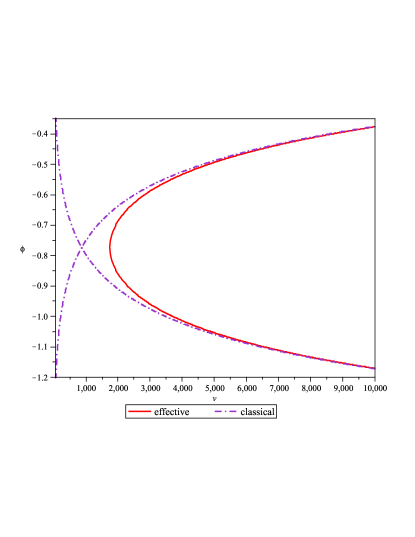
Figure 1: The effective dynamics represented by the observable $v|_{\phi}$ are compared to classical trajectories. In this simulation, the parameters were: $G=\hbar=1\,$, $p_{\phi}=10\,000,$ $\epsilon=0.001\,,\sigma=0.01$ with initial data $v_{o}=100\,000\,$.

On the other hand, the key results discussed in dmy can be carried out similarly. It is easy to see from Eq. (III) that, while the term containing the quantum fluctuations of matter field is qualitatively negligible, the asymptotic behavior of the quantum geometric fluctuations plays a key role for the fate of the universe. By the ansatz $\epsilon=\alpha(r)v^{-r(\phi)}$ with $0\leq r(\phi)\leq 1$, there are great possibilities for the expanding universe to undergo a recollape in the future. The recollape can happen provided $0\leq r<1$ in the large scale limit. Suppose that the semiclassicality of our coherent state is maintained asymtotically. This means that the quantum fluctuation $1/\epsilon$ of $v$ cannot increase as $v$ unboundedly as $v$ approaches infinity. Thus the recollape is in all probability as viewed from the parameter space of $r(\phi)$. For example, in the scenario when $r=0$ asymtotically, besides the quantum bounce when the matter density $\rho$ increases to the Planck scale, the universe would also undergo a recollapse when $\rho$ decreases to $\rho_{\rm coll}\approx\epsilon^{2}\rho^{\prime}_{c}/2$. Therefore, the quantum fluctuations again lead to a cyclic universe in this case. The cyclic universe in this effective scenario is illustrated in Fig. 2.

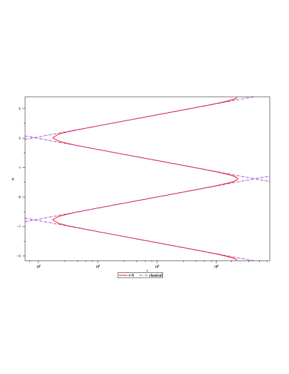
Figure 2: The cyclic model is compared with expanding and contracting classical trajectories. In this simulation, the parameters were: $G=\hbar=1$ , $p_{\phi}=10\,000\,,\epsilon=0.001,\sigma=0.01$ with initial data $v_{o}=100\,000$.

This is an amazing possibility that quantum gravity manifests herself in the large scale cosmology. Nevertheless, the condition that the semiclassicality is maintained in the large scale limit has not been confirmed. Hence further numerical and analytic investigations to the properties of dynamical semiclassical states in the model are still desirable. It should be noted that in some simplified completely solvable models of LQC (see bojow-r and acs ), the dynamical coherent states could be obtained, where $r(\phi)$ approaches $1$ in the large scale limit. While those treatments lead to the quantum dynamics different from ours, they raise caveats to the inferred re-collapse.

In conclusion, the key features of LQC in this model, that the big bang singularity is replaced by a quantum bounce and there are great possibilities for an expanding universe to recollapse, are robust against the quantization ambiguity which we have considered.

APPENDIX

Let us calculate the expectation value of $\hat{C}^{\mathrm{R}}_{\rm grav}$,

$$\langle\hat{C}^{\mathrm{R}}_{\rm grav}\rangle=\frac{(\Psi|\hat{C}^{\mathrm{R}}_{\rm grav}|\Psi\rangle}{\langle\Psi|\Psi\rangle}.$$ (34)

Applying the Poisson resummation formula

$$\sum_{n=-\infty}^{\infty}g(n+x)=\sum_{n=-\infty}^{\infty}e^{2\pi inx}\int_{-\infty}^{\infty}g(y)e^{-2\pi iny}\mathrm{d}y$$ (35)

to the norm of the shadow state (23), one obtains

$$\langle\Psi|\Psi\rangle=\sum_{n\in{\mathbb{Z}}}e^{-\epsilon^{2}n^{2}}=\frac{\sqrt{\pi}}{\epsilon}\left(1+O(e^{-\frac{\pi^{2}}{\epsilon^{2}}})\right).$$ (36)

By Eq. (17), we obtain the action of the gravitational Hamiltonian operator on the shadow state as

$$\hat{C}^{\mathrm{R}}_{\mathrm{grav}}|\Psi\rangle= \sum_{n\in{\mathbb{Z}}}\,e^{-(\epsilon^{2}/2)(n-N)^{2}}e^{-i(n-N)b_{o}}$$

$$\times\Big{[}f^{\prime}_{+}(n+\lambda)|n+\lambda+2\rangle+f^{\prime}_{o}(n+\lambda)|n+\lambda\rangle$$

$$\quad\quad+f^{\prime}_{-}(n+\lambda)|n+\lambda-2\rangle\Big{]}.$$

Then a straightforward calculation shows that

$$(\Psi|\hat{C}^{\mathrm{R}}_{\mathrm{grav}}|\Psi\rangle$$

$$=\sum_{n\in{\mathbb{Z}}}e^{-\epsilon^{2}(n-N)^{2}}\Big{[}2e^{-\epsilon^{2}}\cos(2b_{o})f^{\prime}_{+}(n+\lambda-1)$$

$$\quad\quad\quad\quad\quad\quad\quad\quad-(f^{\prime}_{+}(n+\lambda)+f^{\prime}_{-}(n+\lambda))\Big{]}$$

$$=\frac{27}{4}\sqrt{\frac{8\pi}{6}}\frac{K\ell_{p}}{\gamma^{3/2}}\left[2e^{-\epsilon^{2}}\cos(2b_{o})\bar{S}_{0}-(\bar{S}_{1}+\bar{S}_{-1})\right],$$ (37)

where

$$f^{\prime}_{+}(n)=\frac{27}{4}\sqrt{\frac{8\pi}{6}}\frac{K\ell_{p}}{\gamma^{3/2}}(n+1)\big{(}|n+2|-|n|\big{)},$$

$$f^{\prime}_{-}(n)=\frac{27}{4}\sqrt{\frac{8\pi}{6}}\frac{K\ell_{p}}{\gamma^{3/2}}(n-1)\big{(}|n|-|n-2|\big{)},$$

and we have set

$$\bar{S}_{m}:= \sum_{n\in{\mathbb{Z}}}e^{-\epsilon^{2}(n-N)^{2}}(n+\lambda+m)$$

$$\quad\times\big{(}|n+\lambda+m+1|-|n+\lambda+m-1|\big{)},$$

$$S_{m}:= 2\sum_{n\in{\mathbb{Z}}}e^{-\epsilon^{2}(n-N)^{2}}(n+\lambda+m)$$

$$= 2(N+\lambda+m)\sum_{n\in{\mathbb{Z}}}e^{-\epsilon^{2}n^{2}}.$$

We may bound $|\bar{S}_{m,k}-S_{m}|$ by an exponentially suppressed term:

$$|\bar{S}_{m}-S_{m}|= \,\bigg{|}\sum_{n\in{\mathbb{Z}}}e^{-\epsilon^{2}(n-N)^{2}}(n+\lambda+m)$$

$$\quad\quad\times\big{(}|n+\lambda+m+1|$$

$$\quad\quad\quad-|n+\lambda+m-1|-2\big{)}\bigg{|}$$

$$= \,\bigg{|}\sum_{-1<n+\lambda+m<1}e^{-\epsilon^{2}(n-N)^{2}}(n+\lambda+m)$$

$$\quad\quad\times\big{(}2(n+\lambda+m)-2\big{)}$$

$$\quad\quad+\,4\sum_{n+\lambda+m\leq-1}e^{-\epsilon^{2}(n-N)^{2}}(n+\lambda+m)\bigg{|}$$

$$\leq \,\bigg{|}\sum^{0}_{n+m=-1}e^{-\epsilon^{2}(n-N)^{2}}(n+\lambda+m)$$

$$\quad\quad\times\big{(}2(n+\lambda+m)-2\big{)}\bigg{|}$$

$$\quad\quad+\,4\bigg{|}\sum_{n+m\leq-1}e^{-\epsilon^{2}(n-N)^{2}}(n+m)\bigg{|}$$

$$\quad\quad+4\lambda\sum_{n+m\leq-1}e^{-\epsilon^{2}(n-N)^{2}}$$

$$= \bigg{|}e^{-\epsilon^{2}(m+N)^{2}}\lambda(\lambda-1)$$

$$\,+e^{-\epsilon^{2}(m+N)^{2}}(\lambda-1)(\lambda-2)\bigg{|}$$

$$+\,4\sum_{n\geq 1}e^{-\epsilon^{2}(n+m+N)^{2}}n$$

$$+4\lambda\sum_{n\geq 1}e^{-\epsilon^{2}(n+m+N)^{2}}$$ (38)

Using the Euler-Maclaurin summation, for some positive constant $\alpha$ independent of $N,m$ or $\epsilon$, we obtain:

$$4\sum_{n\geq 1}e^{-\epsilon^{2}(n+m+N)^{2}}n\leq \alpha e^{-N^{2}\epsilon^{2}}+4\int_{1}^{\infty}e^{-\epsilon^{2}(x+m+N)^{2}}x{\mathrm{d}}x$$

$$< \alpha e^{-N^{2}\epsilon^{2}}+\frac{2}{\epsilon^{3}(m+N)}e^{-\epsilon^{2}(m+N)^{2}}.$$ (39)

Hence we obtain $|\bar{S}_{m}-S_{m}|=O(e^{-\epsilon^{2}N^{2}})$. Therefore, we have

$$(\Psi|\hat{C}^{\mathrm{R}}_{\mathrm{grav}}|\Psi\rangle =\frac{27}{4}\sqrt{\frac{8\pi}{6}}\frac{K\ell_{p}}{\gamma^{3/2}}\Big{[}2e^{-\epsilon^{2}}\cos(2b_{o})S_{0}$$

$$\quad\quad-(S_{1}+S_{-1})\Big{]}+O(e^{-N^{2}\epsilon^{2}}).$$ (40)

Finally, we can collect the above terms to calculate the expectation value (34). Using $\langle\Psi|\Psi\rangle=\sum_{n\in{\mathbb{Z}}}e^{-\epsilon^{2}n^{2}}$, we have

$$\langle\hat{C}^{\mathrm{R}}_{\mathrm{grav}}\rangle =27\sqrt{\frac{8\pi}{6}}\frac{K\ell_{p}}{\gamma^{3/2}}(N+\lambda)\left[e^{-\epsilon^{2}}\cos(2b_{o})-1\right]$$

$$\quad+O(e^{-N^{2}\epsilon^{2}})$$

$$=-54\sqrt{\frac{8\pi}{6}}\frac{K\ell_{p}}{\gamma^{3/2}}|v_{o}|\left[e^{-\epsilon^{2}}\sin^{2}b_{o}+\frac{1}{2}(1-e^{-\epsilon^{2}})\right]$$

$$\quad\quad+O(e^{-N^{2}\epsilon^{2}}).$$ (41)

References

- (1) M. Bojowald, Phys. Rev. Lett. 86, 5227 (2001).
- (2) A. Ashtekar, T. Powlowski and P. Singh, Phys. Rev. Lett. 96, 141301 (2006).
- (3) A. Ashtekar, T. Pawlowski and P. Singh, Phys. Rev. D 74, 084003 (2006).
- (4) M. Bojowald, Living Rev. Rel. 8, 11 (2005).
- (5) A. Ashtekar and J. Lewandowski, Class. Quantum Grav. 21, R53 (2004).
- (6) C. Rovelli, Quantum Gravity, (Cambridge University Press, Cambridge, England, 2004).
- (7) T. Thiemann, Modern Canonical Quantum General Relativity, (Cambridge University Press, Cambridge, England, 2007).
- (8) M. Han, Y. Ma and W. Huang, Int. J. Mod. Phys. D 16, 1397 (2007).
- (9) M. Bojowald, Phys. Rev. D 75, 081301(R) (2007).
- (10) A. Ashtekar, Loop quantum cosmology: an overview, arXiv:0812.0177.
- (11) Y. Ding, Y. Ma and J. Yang, Phys. Rev. Lett. 102, 051301 (2009).
- (12) A. Ashtekar, M. Bojowald and J. Lewandowski, Adv. Theor. Math. Phys. 7, 233 (2003).
- (13) V. Taveras, Phys. Rev. D 78, 064072 (2008).
- (14) A. Ashtekar, S. Fairhurst and J. Willis, Class. Quantum Grav. 20, 1031 (2003); J. Willis, PhD Thesis, (Pennsylvania State University, 2004).
- (15) A. Ashtekar, A. Corichi and P. Singh, Phys. Rev. D 77, 024046 (2008).