Grain Growth and Density Distribution of the Youngest Protostellar Systems

Abstract

We present dust opacity spectral indexes ($\beta$) of the youngest protostellar systems (so-called Class 0 sources), L1448 IRS 2, L1448 IRS 3, and L1157, obtained between the $\lambda=1.3$ mm and 2.7 mm continua, using the Combined Array for Research in Millimeter-wave Astronomy (CARMA). The unprecedented compact configuration and image fidelity of CARMA allow a better detection of the dust continuum emission from Class 0 sources, with a less serious missing flux problem normally associated with interferometry. Through visibility-modeling at both $\lambda=1.3$ mm and 2.7 mm simultaneously, as well as image- and visibility-comparison, we show that $\beta$ of the three Class 0 sources are around or smaller than 1, indicating that dust grains have already significantly grown at the Class 0 stage. In addition, we find a radial dependence of $\beta$, which implies faster grain growth in the denser central regions and/or dust segregation. Density distributions of the Class 0 sources are also addressed by visibility-modeling.

1. Introduction

Although dust grains are only about one hundredth of the interstellar medium by mass, they play crucial roles for star formation, planet formation, and furthermore the origin of life. They are essential places to form and store molecules, and they are the main ingredient to form terrestrial planets, as well as playing a role in the heating and cooling mechanisms during star and planet formation.

The dust opacity spectral index ($\beta$) is related to dust properties. It depends on dust grain sizes, compositions, and shapes (e.g., Pollack et al., 1994; Draine, 2006). In particular, it is largely sensitive to grain sizes; larger grains give smaller $\beta$ (e.g., Draine, 2006). Many observational studies at infrared and millimeter wavelengths toward T Tauri circumstellar disks have reported smaller values of $\beta$ ($\sim 1.0$) (e.g., Andrews & Williams, 2007) compared to that of the interstellar medium ($\sim 1.7$) (Finkbeiner et al., 1999; Li & Draine, 2001). In the sense that dust grains may develop terrestrial planets, it is very encouraging to see signatures of larger dust grains in T Tauri disks, evolved young stellar objects (YSOs), compared to grains in the interstellar medium.

However, it is not clear when the dust grain growth responsible for the opacity spectral index $\beta\sim 1$ mainly occurs. For example, while Andrews & Williams (2005) reported grain growth along the YSO evolution from Class I to Class II, using spectral energy distributions over $\lambda=1.3$ mm and submillimeter data, Natta et al. (2007) did not find such a tendency (a systematic variation of $\beta$). To distinguish when dust grains mainly grow up to the sizes for $\beta\sim 1$, Class 0 YSOs are the best targets to examine. Class 0 YSOs are at the starting point of low-mass star formation and they are well defined. They have more massive envelopes than or comparably massive envelopes to their central compact objects (e.g., Andre et al., 1993). They are also characterized with well-developed bipolar outflows. Earlier stages such as starless cores might be another good target but they are hardly confined. Their physical conditions including age have a much larger scatter than Class 0 sources. In addition, they are not all expected to form stars.

In fact, no definitive answer has been given to the opacity spectral index $\beta$ of Class 0 sources so far. It is another reason that this study is needed beyond the grain growth point of view. There are some previous studies about the flux density spectral indexes of Class 0 sources, which are related to the dust opacity spectral indexes, although they have not focused on dust properties (e.g., Hogerheijde & Sandell, 2000; Shirley et al., 2000). However, these studies used submillimeter to 1.3 mm wavelengths, which is near the range of peak intensities at envelope temperatures ($\sim 30$ K), so the Rayleigh-Jeans approximation is invalid. In that case, the estimate of $\beta$ is sensitive to the envelope temperature, which causes relatively large uncertainties in the $\beta$ estimate. In addition, optical thickness can cause another uncertainty, since Class 0 YSO envelopes can be optically thick at submillimeter wavelengths. On the other hand, Harvey et al. (2003) obtained $\beta\sim 0.8$ toward the Class 0 YSO B335 using $\lambda=1.2$ mm and 3 mm interferometric data, while carrying out modeling to test density distribution models of star formation. However, they did not have a good data set with comparable uv coverage at both wavelengths to discuss the $\beta$ in detail. In other words, there are no reliable $\beta$ estimates of Class 0 YSOs. As a result, many studies to estimate masses from spectral energy distributions (SEDs) and/or to constrain density distributions have assumed $\beta\sim 1$ (e.g., Looney et al., 2003) or considered a possible range of $\beta$ (e.g., $\beta=1-2$, Chandler & Richer, 2000).

Radio interferometry at millimeter wavelengths is the best means to investigate the $\beta$ of Class 0 YSOs. As mentioned, optical thickness and dust temperature issues cause large uncertainties at shorter wavelengths. On the other hand, contamination of non-thermal continuum increases with wavelength, so it is not negligible at longer centimeter wavelengths. In addition, considering envelope sizes of Class 0 YSOs and their environments (normally they are within extended molecular clouds), single dish observations are not appropriate due to their lack of angular resolution and the contamination of molecular clouds. In contrast, interferometers provide high angular resolution and resolve out the emission from the large-scale molecular cloud. However, they may also resolve out emission from the Class 0 envelopes. This is caused by limited uv coverage, particularly due to the absence of short baselines and zero-spacing. For these reasons, interferometers with good uv coverage are required. The recently commissioned Combined Array for Research in Millimeter-wave Astronomy (CARMA) provides the best opportunity with its unprecedented compact configuration and image fidelity (Woody et al., 2004).

In this paper, we present dust opacity spectral indexes $\beta$ of Class 0 sources (L1448 IRS 2, L1448 IRS 3, and L1157) in order to tackle when the dust grain growth responsible for $\beta\sim 1$ mainly occurs: before or after the Class 0 stage. We do a parametric modeling in uv space to address the $\beta$ values, as well as image and visibility comparisons. In addition, we examine power-law density indexes via modeling. First, we discuss our observations and data reduction, focusing on how well our CARMA data incorporate with this study. Afterward, we show our results in images, uv visibilities, and visibility modelings. At the end, we discuss the implications of our results.

2. Target YSOs

We have carried out observations of three Class 0 YSO regions (L1448 IRS 2, L1448 IRS 3, and L1157) using CARMA in the $\lambda=1.3$ mm and 2.7 mm continuum. These three targets are well defined as Class 0 YSOs by previous studies (e.g., Shirley et al., 2000; O’Linger et al., 1999). L1448 IRS 2 and IRS 3 are located in the dark cloud L1448 of the Perseus molecular cloud complex at a distance of 250 pc. They were first revealed by IRAS observations (Bachiller & Cernicharo, 1986). L1448 IRS 3 is the brightest infrared source in the dark cloud and has three Class 0 sources (3A, 3B, and 3C), revealed by radio interferometric observations (Curiel et al., 1990; Terebey & Padgett, 1997; Looney et al., 2000). Kwon et al. (2006) also studied the binary system of 3A and 3B, the two interacting bipolar outflows, and the magnetic field in the region, using polarimetric observations of the Berkeley Illinois Maryland Association (BIMA) array in the $\lambda=1.3$ mm continuum and CO $J=2\rightarrow 1$ transition line.

On the other hand, L1448 IRS 2 at $\sim 3\arcmin$ west of IRS 3 has not been focused on very much due to its weaker brightness. However, O’Linger et al. (1999) identified it as a Class 0 YSO, using far-infrared up to millimeter continuum observations. In addition, recent deep Spitzer Space Telescope (SST) IRAC observations have shown a large bipolar outflow spanning over $5\arcmin$ (Tobin et al., 2007). CARMA observations in CO $J=2\rightarrow 1$ and $J=1\rightarrow 0$ transitions also show a well-developed bipolar outflow (Kwon et al., 2009).

L1157 is a dark cloud in Cepheus. The distance is not well known but it is arguably about 250 pc (Looney et al., 2007). Its envelope and large bipolar outflow have been studied by radio single dish and interferometric observations (e.g., Bachiller et al., 2001; Gueth et al., 2003; Beltrán et al., 2004). The bipolar outflow is known as chemically active, since various molecules have been detected and interestingly there is an abundance gradient that cannot be explained purely by excitation temperature differences (Bachiller et al., 2001). Recently, a flattened envelope has been detected in absorption against polycyclic aromatic hydrocarbon (PAH) background emission by deep SST IRAC observations (Looney et al., 2007).

3. Observations and Data Reduction

We have carried out $\lambda=$ 1.3 mm and 2.7 mm continuum observations towards three Class 0 sources, L1448 IRS 2, L1448 IRS 3, and L1157, using CARMA (Woody et al., 2004), which is a recently commissioned millimeter array, combining the BIMA and OVRO (Owens Valley Radio Observatory). It consists of 6 elements of 10.4 m antennas and 9 elements of 6.1 m antennas. In order to achieve a similar synthesized beam at the two wavelengths, the $\lambda=$ 1.3 mm and 2.7 mm continuum data have been taken in the most compact E configuration and the D configuration, respectively. These two combinations of wavelengths and array configurations provide well matched synthesized beams, about $5\arcsec\times 5\arcsec$.

This moderately matched beam size at these two wavelengths has not been achievable before CARMA. In interferometric observations, while high angular resolution can be obtained via increasing baselines of antenna elements, there is the usual missing flux problem. This is because interferometric observations are only sensitive to size scales corresponding to the uv coverage. To mitigate the missing flux issue, we need either an additive single dish observation or well-defined uv coverage with short baselines. From this point of view, the most compact CARMA E configuration is just right to study Class 0 envelope structures, since the canonical size of Class 0 source envelopes is several thousands of AU corresponding to a few tens of arc-seconds in most nearby star forming regions (e.g., the Perseus molecular cloud at a distance of 250 pc). The E configuration provides baselines from $\sim 6$ m to $\sim 60$ m ($\sim 4.6-46$ k$\lambda$ at $\lambda=1.3$ mm), which result in a synthesized beam (angular resolution) of about $5\arcsec\times 5\arcsec$. A simulation shows that our data uv coverage recovers fluxes well ($>50$%) towards extended features about up to 4 times the synthesized beam size.

CARMA has a couple of special features to realize the most compact E configuration. One is an anti-collision system installed on the 6.1 m antennas, which are located in the inner region of the configuration. Antennas stop whenever they are in a danger of collision. The other feature is the coordinated movement. In larger configurations, D, C, and B configurations, antennas diagonally move (simultaneously in azimuth and elevation) to reach a target. However, in E configuration they go to a high elevation first and move in azimuth followed by a movement to arrive at a designated elevation, to reduce the collisional situations.

The $\lambda=2.7$ mm continuum was observed in the D-like commissioning configuration of 2006 fall and winter and D configuration of 2007 summer, while the $\lambda=1.3$ mm continuum was obtained in the E configuration of 2007 summer. Each data set was taken with one or two double-side bands of a 500 MHz bandwidth in each single-side band for the continuum observations. Two or one extra bands were assigned to a CO rotational transition ($J=2\rightarrow 1$ or $J=1\rightarrow 0$). The CO rotational transition data are presented in another paper with other molecular transition data. The details of each observation are listed in Table 1. Two and three pointing mosaics have been done to better cover the larger bipolar outflow regions for the $\textrm{CO}~{}J=2\rightarrow 1$ transition towards L1448 IRS 3 and L1157, respectively, at $\lambda=1.3$ mm. For this study, the northwest pointing data of L1448 IRS 3 and the central pointing data of L1157 were used.

The Multichannel Image Reconstruction, Image Analysis, and Display (MIRIAD, Sault et al., 1995) tools have been employed to reduce and analyze data. In addition to normal procedures (linelength, bandpass, flux, and gain calibrations), shadow-defected data have been flagged in the E configuration data. Shadowing indicates cases of an antenna’s line-of-sight interrupted by other antennas and usually appears in low elevation observations of compact configurations. The normal effects of shadowing are reduction and distortion of incident antenna power and abnormal gain jumps. Therefore, to obtain reliable results the shadow-defected data were flagged in the compact E configuration.

Further special attention needs to be given on flux calibration for studies involving flux comparison between different wavelengths like this study. To minimize errors caused by primary flux calibrators, we used the same flux calibrator (Uranus) at both wavelengths except L1157, which used MWC349 at $\lambda=1.3$ mm and Mars at $\lambda=2.7$ mm. We expect 15% and 10% uncertainties of flux calibrations at $\lambda=1.3$ mm and 2.7 mm, respectively, based on the CARMA commissioning task of flux calibration. During a commissioning period extending to longer than 4 months, 12 calibrator (quasar) fluxes had been monitored by CARMA. As a result, the least varying case showed about 13% deviation in flux. When considering the intrinsic variability of quasars, it is expected that CARMA flux calibrations have about $10-15$% uncertainties. As a result, we consider 15% and 10% uncertainties at $\lambda=1.3$ mm and 2.7 mm, respectively.

In addition, we make synthesized beam sizes the same as possible at both wavelengths, using weighting and tapering schemes, in order to minimize the beam size effect on the flux comparison. After proper weighting and tapering schemes, we could match the beam sizes to within 1%. The details of applied weighting and tapering schemes are listed in Table 2 with final synthesized beams. Briggs’ robust parameter is used (Briggs, 1995), which is a knob to provide intermediate weighting between natural and uniform weighting. The parameter of $2$ gives a weighting close to natural weighting and $-2$ close to uniform weighting.

4. Observation Results

4.1. Dust opacity spectral index maps

Total flux ($F_{\nu}$) of the thermal dust continuum emission represents the total mass ($M_{T}$) of the source, if the source is optically thin at the observational frequencies,

$$F_{\nu}\approx\kappa_{\nu}\,B_{\nu}(T_{d})\,\frac{M_{T}}{D^{2}},$$ (1)

where $\kappa_{\nu}$, $B_{\nu}(T_{d})$, $M_{T}$, and $D$ are opacity (mass absorption coefficient) of the dust grains, blackbody radiation intensity of a dust temperature $T_{d}$, total mass, and distance to the source, respectively. The opacity of dust grains ($\kappa_{\nu}$) depends on dust properties such as sizes, components, and shapes. If the dependence is simple, for example a power law ($\kappa_{\nu}\varpropto\nu^{\beta}$), the dust grain properties can be studied by observations at two frequencies. In addition, in the case that the Rayleigh-Jeans approximation of blackbody radiation is applicable ($h\nu\ll kT$), the relationship between spectral indexes of the observed flux densities ($\alpha$) and spectral indexes of the dust grain opacity ($\beta$) is simply,

$$F_{\nu} \approx F_{\nu_{0}}\Big{(}\frac{\nu}{\nu_{0}}\Big{)}^{\alpha}$$

$$F_{\nu} \approx \kappa_{\nu}\,B_{\nu}(T_{d})\,\frac{M_{T}}{D^{2}}$$

$$\approx \kappa_{\nu_{0}}\Big{(}\frac{\nu}{\nu_{0}}\Big{)}^{\beta}\,\,\frac{2kT_{d}}{c^{2}}\,\nu^{2}\,\frac{M_{T}}{D^{2}}$$

$$\textrm{therefore}~{}~{}~{}~{}~{}\alpha \approx \beta+2.$$ (2)

Note that this relation is valid only in the optically thin assumption and the Rayleigh-Jeans approximation.

Draine (2006) showed that $\beta$ mainly depends on the size distribution of dust grains rather than their components and shapes; small $\beta$ ($\sim 1$) is likely indicating dust grain size distribution up to $3\lambda$. Since our observations are up to 3 mm, $\beta\sim 1$ would suggest a grain size distribution up to about 1 cm.

Figure 1 presents maps of L1448 IRS 2, L1448 IRS 3, and L1157. Dust continuum maps at $\lambda=1.3$ mm and $\lambda=2.7$ mm have been separately constructed using different weightings and taperings as described in § 3 and Table 2 in order to have as similar synthesized beams as possible at the two wavelengths. Afterwards $\beta$ values of each source have been calculated using the two continuum images. Only regions above three signal-to-noise ratio (SNR) levels on the both maps have been used to derive $\beta$ assuming

$$\beta=\frac{\log(F(\nu_{1})/F(\nu_{0}))}{\log(\nu_{1}/\nu_{0})}-2,$$ (3)

where $\nu_{1}$ and $\nu_{0}$ are frequencies corresponding to $\lambda=1.3$ mm and $\lambda=2.7$ mm data, as listed in Table 2. Note that the Rayleigh-Jeans approximation and the optically thin assumption are used. In the case of an average dust temperature of about 30 K, the upper limit of frequencies to which the Rayleigh-Jeans approximation can be applied is about 625 GHz. Since the higher frequency of our data is about 230 GHz, the assumption is valid for this study. However, caution should be taken in $\beta$ comparison at submillimeter wavelengths for cold objects such as the Class 0 YSO envelopes.

As shown in Figure 1, most $\beta$ values in the three targets are less than 1. For a convenient comparison, the same gray scales have been adopted for all three maps. The actual ranges of $\beta$ values are in Table 3 with the averages. As listed in the table, the maximum values are larger than 1.0. However, those large $\beta$ values appear only on a few pixels of source boundaries, which may be due to contamination from ambient clouds. $\beta$ and its averages in most regions of the three sources are similar to or less than 1. In the case of L1448 IRS 3, in which three Class 0 sources (3A, 3B, and 3C) exist, $\beta$ values corresponding to the three sources are separately listed in Table 3. Like the other targets, these three sources of L1448 IRS 3 have $\beta$ around or less than 1. The L1448 IRS 3A and 3B fluxes are obtained simply by cutting the protuberance in Figure 1. Table 3 also has $\beta$ values obtained from the total fluxes at the two wavelengths, which have been estimated in source regions limited by the three SNR threshold at both wavelengths. All sources except L1448 IRS 3B have $\beta$ values comparable to the mean values of the $\beta$ maps.

Another feature to note is that there are $\beta$ gradients with radius in all sources. L1157 has a smaller $\beta$ in the northeast-to-southwest direction, roughly consistent with the $\lambda=1.3$ mm and 2.7 mm results of Beltrán et al. (2004). However, it is noteworthy that they restored their two images with an identical beam size without any weighting schemes, which could cause a biased result due to different uv coverage of the two wavelength data. The radial dependence of $\beta$ is better shown in § 4.2 and is discussed in detail for the L1448 IRS 3B case via modeling in § 6

4.2. Visibility data comparison

We have also examined $\beta$ values in uv space, which is the Fourier transformed space of an image. Data of interferometric observations are obtained in uv space and called uv visibilities or just visibilities. To obtain a sky intensity distribution, inverse Fourier transformation and deconvolution (e.g., CLEANING algorithm) are employed (e.g., Thompson et al., 2001). However, limited uv coverage causes difficulties, i.e., the deconvolution introduces systematic biases, especially for non-point, extended sources. One of the best ways to overcome this difficulty is to investigate the visibility data in uv space instead.

The results of $\beta$ calculated in uv space are displayed in Figure 2. Visibilities have been vector-averaged in annuli. Since the envelope structures from our observations are spherical, the annulus averaging is valid. The annulus bin sizes are $\sim 3.1$ k$\lambda$ except when the SNR is too low, usually at the relatively longer baselines. This is most noticeable in L1157 at $\lambda=2.7$ mm. Although the uv coverage is comparable at both wavelengths, the lower SNR at $\lambda=2.7$ mm requires larger bins. The $\beta$ values are calculated at the $\lambda=1.3$ mm bins with $\lambda=2.7$ mm visibilities linearly interpolated using the nearest bin values. When the $\lambda=1.3$ mm bin center is beyond last $\lambda=2.7$ mm bin center (extrapolation case), then the nearest bin value for $\lambda=2.7$ mm is used.

In the case of L1448 IRS 3, only 3B is considered for the $\beta$ calculation in uv space. The other two objects, 3A and 3C, are too small and weak to carry out the calculation. On the other hand, 3A and 3C should be removed from the visibilities to obtain the 3B data. Using the MIRIAD task UVMODEL and image models excluding the two components, we subtracted the 3A and 3C visibilities at both $\lambda=1.3$ mm and $\lambda=2.7$ mm separately. In addition, since the $\lambda=1.3$ mm data set has been taken with two pointings offset from the center, we compensated the primary beam sensitivity loss using a UVMODEL multiplication.

In Figure 2, the upper panels show amplitudes of $\lambda=1.3$ mm (open squares) and $\lambda=2.7$ mm cases (open triangles). The error bars represent the statistical standard errors in each bin. The solid and dashed lines present the best fit models described in § 5 and Figure 3. The lower panels show $\beta$ values with uv distance, calculated by equation (3). The open circles indicate $\beta$ values calculated from the uv visibilities shown on the upper panels. The error bars with caps on the open circles represent $\beta$ value ranges corresponding to the statistical amplitude errors of the upper panels. The filled circles and error bars without caps show the effect that the absolute flux calibration uncertainty has on the calculation of $\beta$. We adopt 15% flux calibration uncertainties for $\lambda=1.3$ mm data and 10% for $\lambda=2.7$ mm data, as discussed in § 3. The larger $\beta$ points indicate the case in which 15% higher fluxes at $\lambda=1.3$ mm and 10% lower fluxes at $\lambda=2.7$ mm are considered and vise verse for the lower $\beta$ points. The $\beta$ ranges are around $\pm 0.35$, as $\textrm{log}(1.15/0.90)/\textrm{log}(\nu_{1}/\nu_{0})\approx 0.35$ where $\nu_{1}/\nu_{0}\approx 2$ (refer to eq. 3).

Two main features should be noted in Figure 2. One point is that the $\beta$ values are around 1 or less than 1 in all three objects. It is arguably true even when considering the absolute flux calibration uncertainties. The other point is the radial dependences of $\beta$. In L1448 IRS 2 and L1157, $\beta$ arguably decreases on smaller scales (larger uv distances). L1448 IRS 3B, however, distinctly presents a radial dependence. The $\beta$ variation is fit with the logarithmic function of $\beta(\zeta)=1.0-0.57~{}\textrm{log}(\zeta)$, where $\zeta$ is the uv distance in units of k$\lambda$. When assuming power-law distributions of density and temperature of envelopes as discussed in § 5, the distributions of the intensity integrated along line-of-sight as well as the radial intensity follow a power-law under the optically thin assumption and Rayleigh-Jeans approximation (Adams, 1991). When ignoring primary beam effects of interferometers and assuming infinite size envelopes, the visibilities are also in a power-law (e.g. Harvey et al., 2003; Looney et al., 2003). As $\beta$ is obtained from equation (3) here, we assume a logarithmic function of $\beta(\zeta)$. There are a few possible interpretations to explain this radial dependence of $\beta$. It could be caused by increasing the fraction of optically thick emission on smaller scales due to the denser central region. Beckwith et al. (1990) discussed that the optically thick emission fraction ($\Delta$) decreases $\beta$ by a factor of ($1+\Delta$), i.e., $\beta\simeq\beta_{0}/(1+\Delta)$. Similarly, it could be due to an optically thick, unresolved, deeply embedded disk structure at the center. On the other hand, it could indicate a faster grain growth in the denser central region or dust grain segregation suggested by some star formation theories, for example, ambipolar diffusion in magnetically supported molecular cloud (Ciolek & Mouschovias, 1996). The radial dependence is discussed in more detail in § 6.

5. Modeling in uv space

As mentioned in § 4.2, images of extended features constructed from interferometric observations may be biased due to limited uv coverage. In contrast, comparing visibility data against source models transformed to the visibility plane (including the primary beam modification, Fourier transformation, and visibility sampling), is not prone to these imaging deconvolution biases. Therefore, we carry out envelope modeling in uv space rather than in image space. In other words, we compare observation visibilities with model visibilities sampled over the observation uv coverage, after obtaining uv models by the Fourier-transformation of image models.

We assume that the temperature distribution of dust grains is in radiative equilibrium with the central protostar, ignoring heating by gas and cosmic rays (Spitzer, 1978, p 193):

$$c\int_{0}^{\infty}Q_{a}(\nu)\,u_{\nu}\,d\nu=4\pi\int_{0}^{\infty}Q_{a}(\nu)\,B_{\nu}(T_{d})\,d\nu,$$ (4)

where $Q_{a}(\nu)$, $u_{\nu}$, $B_{\nu}(T_{d})$, and c are absorption efficiency factor, radiation energy density, black body radiation intensity of temperature $T_{d}$, and speed of light, respectively. The radiation energy density ($u_{\nu}$) at a distance $r$ from the center can be expressed as $\pi B_{\nu}(T_{*})\,R_{*}^{2}/r^{2}$, where $T_{*}$ and $R_{*}$ are an effective temperature and a radius of a central protostar. Assuming $Q_{a}(\nu)\propto\nu^{\beta}$, equation (4) gives a temperature distribution of dust grains (Beckwith et al., 1990),

$$T_{d}(r)=T_{*}\,\Big{(}\frac{1}{2}\frac{R_{\ast}}{r}\Big{)}^{2/(4+\beta)}.$$ (5)

Again, $\beta$ is the dust grain opacity spectral index ($\kappa_{\nu}=\kappa_{0}(\nu/\nu_{0})^{\beta}$). This equation can also be formulated with a grain temperature $T_{0}$ at a distance $R_{0}$ from the central protostellar luminosity $L_{0}$, as (e.g., Looney et al., 2003)

$$T_{d}(r)=T_{0}\,\Big{(}\frac{R_{0}}{r}\Big{)}^{2/(4+\beta)}\Big{(}\frac{L_{*}}{L_{0}}\Big{)}^{1/(4+\beta)}.$$ (6)

Although the inner region, which might be optically thick, could have a sharper temperature gradient than this relation (e.g., Wolfire & Cassinelli, 1986; Looney et al., 2003), it is limited at the very central region, and our results are not sensitive to the possibility, as further discussed in § 6.

Some previous studies (e.g., Harvey et al., 2003) considered the external heating by the interstellar radiation field, using a temperature lower limit of 10 K. However, we do not explicitly include this effect, since the temperature lower limit is uncertain and the lowest temperature of our modeling is comparable, about 7.3 K at $r=7000$ AU when adopting $T_{0}=100$ K at $r=10$ AU. In addition, tests show that the temperature lower limit does not change our results, as previous studies also reported (e.g., Harvey et al., 2003). The outer envelope heated externally by the interstellar radiation field would be the main intensity component in sources without any central heating objects, but in Class 0 YSOs the central high temperature region drives the emission. Besides, interferometric observations are not so sensitive to the outer envelope, where the effect of the temperature lower limit is largest.

The power-law density distribution is assumed for envelopes, $\rho(r)=\rho_{0}(r/r_{0})^{-p}$. Therefore, the intensity of envelopes on the plane of the sky is calculated as

$$I_{\nu}=\int B_{\nu}(T_{d}(r))~{}e^{-\tau_{\nu}}~{}d\tau_{\nu}=\int B_{\nu}(T_{d}(r))~{}e^{-\tau_{\nu}}~{}\rho(r)~{}\kappa_{\nu}~{}dL,$$ (7)

where L indicates the line-of-sight from the observer and the optical depth $\tau_{\nu}=\int_{0}^{L}\kappa_{\nu}~{}\rho(r)~{}dL^{\prime}$. Spherical envelopes with an outer radius of $R_{out}$ and with an inner hole of a radius of $R_{in}$ are assumed. Therefore, the density distribution can be expressed with the total envelope mass $M_{T}$ (when $p\neq 3$) as

$$M_{T} = \int_{R_{in}}^{R_{out}}\rho(r)~{}4\pi r^{2}~{}dr$$ (8)

$$= \frac{4\pi}{3-p}(R_{out}\,\!^{3-p}-R_{in}\,\!^{3-p})~{}\rho_{0}\,r_{0}\,\!^{p}$$

$$\rho(r) = \rho_{0}\,r_{0}\,\!^{p}~{}r^{-p}$$ (9)

$$= M_{T}~{}\frac{3-p}{4\pi}(R_{out}\,\!^{3-p}-R_{in}\,\!^{3-p})^{-1}~{}r^{-p}.$$

Substituting the density expression with the total envelope mass into the optical depth of equation (7) shows a coupling of $M_{T}$ and $\kappa_{0}$ — in the case that the envelope is optically thin and the Rayleigh-Jeans approximation ($B_{\nu}(T_{d}(r))\approx 2kT_{d}(r)/\lambda^{2}$) is valid, $T_{0}$ is also coupled. Normally the envelopes of this stage YSO are optically thin in the $\lambda=1.3$ mm and $2.7$ mm continua except the very central regions (within a few tens of AU) and the Rayleigh-Jeans approximation is applicable, which means that the $M_{T}$, $\kappa_{0}$, and $T_{0}$ are all likely coupled. However, note that the optically thin assumption and Rayleigh-Jeans approximation, which are assumed in $\beta$ calculations of observational data in § 4.1 and § 4.2, are not assumed in the modeling to avoid biases. Here we just intend to point out that the three parameters are likely to be coupled.

After constructing intensity image models, they are corrected by three different CARMA primary beams, which correspond to baselines of two 10.4 m antennas, two 6.1 m antennas, and 10.4 m and 6.1 m antennas. The three primary-beam corrected images are Fourier-transformed into uv space and model visibilities are sampled over the actual observational uv coverage of the three different baselines. Comparison between model and observation visibilities is done by vector averaged values in annulus bins. Although bipolar outflows at this stage carve a cavity (e.g., Seale & Looney, 2008), the effect is minor (Chandler & Richer, 2000), especially at our intermediate angular resolution. In addition to the bipolar outflow effect, envelopes might be clumpy. However, the effect on our modeling is also insignificant, since the angular resolution of our data is intermediate and annulus-averaged values are used for the comparison of models and data.

Parameters involved in our modeling are $p$ (power-law density index), $\beta$ (opacity spectral index), $M_{T}$ (envelope total mass), $\kappa_{0}$ (opacity coefficient at $\nu_{0}$), $T_{0}$ (grain temperature at $R_{0}$), $R_{in}$ and $R_{out}$ (inner and outer radii of envelopes), and $F_{pt}$ (a central point source flux at $\lambda=2.7$ mm). Among these, two parameters are fixed: $\kappa_{0}=0.0114$ cm² g^-1 at $\nu_{0}=230$ GHz and $T_{0}=100$ K at $R_{0}=10$ AU. As discussed, the $\kappa_{0}$ and $M_{T}$ are coupled (and so $T_{0}$ is mostly), so we cannot well constrain these parameters simultaneously. The $T_{0}$ at $R_{0}$ corresponds to a central object luminosity of 1.67 $L_{\sun}$ and the $\kappa_{0}$ at $\nu=230~{}\textrm{GHz}$ is the average of $\beta=1$ and $2$ cases in $\kappa_{\nu}=0.1\,(\nu/1200~{}\textrm{GHz})^{\beta}$, assuming a gas-to-dust mass ratio of 100 (e.g., Hildebrand, 1983; Beckwith et al., 1990). Ossenkopf & Henning (1994) also reported $\kappa\approx 0.01$ cm² g^-1 at $\lambda=1.3$ mm for dense protostellar cores via dust coagulation model calculation, when using a gas-to-dust mass ratio of 100. Note that $\kappa_{0}$ is not very well known and has a large uncertainty (e.g., Hildebrand, 1983; Beckwith & Sargent, 1991) so we need to pay attention to the fact that the total mass $M_{T}$ could have a large uncertainty. $M_{T}$ can also be scaled by the presumed $T_{0}$.

The central point source flux ($F_{pt}$) is designed to simulate an unresolved central disk structure. We assumed that the point sources are optically thick so that the flux density spectral index is 2 under the Rayleigh-Jeans approximation, meaning $\beta=0$. In the case of L1448 IRS 2 there is no point source required, since there is no flat visibility amplitude on the small scales, particularly at $\lambda=1.3$ mm in Figure 2. It may indicate that the central disk structure of the source is not so significant. In contrast, L1157 has a flat profile on the small scales, which means a compact structure at the center. Therefore, a point source is adopted to fit the data. Indeed, Beltrán et al. (2004) reported a compact component (size $<1\arcsec$) of 25 mJy and 78 mJy at $\lambda=2.7$ mm and 1.3 mm, respectively. On the other hand, the point source of L1448 IRS 3B was applied for a different reason: to simulate a radial dependence of $\beta$. As shown in Figure 2, there is a clear radial dependence of $\beta$, which results in no good fits with a constant $\beta$ over all scales. It is why an optically thick point source is considered, although there is no flat feature on the small scales. Note that even higher angular resolution observations have not detected such a point source signature (Looney et al., 2003). We further discuss the $\beta$ radial dependence of L1448 IRS 3B in § 6.

In order to find good fit models, we search grids of parameters, $p$, $\beta$, $M_{T}$, $R_{in}$, $R_{out}$, and $F_{pt}$. Parameter set information of the three sources is listed in Table 4. On each grid point of parameters, the reduced $\chi^{2}$ ($\chi_{\nu}^{2}$) has been calculated. The two wavelength data were used simultaneously for fitting. Note that the absolute $\chi_{\nu}^{2}$ values particularly in L1448 IRS 3B ($\sim 8.7$) are large, compared to L1448 IRS 2 ($\sim 1.6$) and L1157 ($\sim 1.5$). This is because the relatively small standard errors due to the high brightness of L1448 IRS 3B make fitting very difficult. The L1448 IRS 3B data may have imperfect exclusion of the companion L1448 IRS 3A, which might cause a difficulty in fitting. However, it is unlikely to be the main effect, since the companion is relatively weak and we subtracted the component as mentioned in § 4.2. In addition, the vector averaging in annuli minimizes the effect. On the other hand, it may indicate that the simple power-law model is not appropriate to explain high SNR observations (e.g., Chiang et al., 2008).

We adopt a likelihood calculation to constrain $p$ and $\beta$, instead of reporting large ranges of each parameter to fit the data. Reporting good fit parameter ranges could bias the impression of the results, since each parameter value in the range comes from different combinations of the other parameters. The likelihood function we adopt is $\textrm{exp}(-\chi_{\nu}^{2}/2)$, since the annulus averaged visibilities have a Gaussian distribution based on the central limit theorem. As we want to constrain $p$ and $\beta$, the likelihoods of all grid points with common $p$ and $\beta$ are summed. The sum now indicates the likelihood of a set of $p$ and $\beta$. Finally, it is normalized by the total sum of the likelihoods in each plot of Figure 3, which means that the plots are comparable to probability density distributions of $p$ and $\beta$. Note that we do not consider the absolute flux calibration uncertainties for fitting. In other words, we use data points marked with open symbols in Figure 2. Note that while systematic changes of absolute fluxes in the same direction at both $\lambda=1.3$ mm and $2.7$ mm affect the total mass $M_{T}$, the opposite direction changes mainly influence $\beta$. We estimate that the maximum $\beta$ ranges caused by the absolute flux calibration uncertainties are $\pm 0.35$, as mentioned in § 4.2.

We present the most likely $\beta$ and $p$ in Figure 3. As clearly shown in the figure, $\beta$ of the three sources are most likely to be around 1 even in the modeling without the optically thin assumption and Rayleigh-Jeans approximation. These are the first clear modeling results showing the $\beta$ of Class 0 YSOs. The contours in Figure 3 indicate likelihood levels of 90% down to 10% of the peak in steps of 10% and the triangles and circles mark the $p$ and $\beta$ pairs of the best fit models and likelihood weighted averages of individual parameters, respectively. Note that, therefore, the combinations of the weighted averages are not necessarily the best fit. Since a model with a point source is not the best one for L1448 IRS 3B, its contours are drawn in dashed lines. (The best model is discussed in § 6 and displayed in Figure 6.) The broader distribution in $p$ of L1157 is due to the adopted point sources. As having a point source implies a density gradient, it lowers the density index. The two dotted contours in the L1157 plot present 90% and 80% of the peak likelihood based on all models in the whole range of the point source fluxes $F_{pt}$ ($0.000-0.035$ Jy at $\lambda=2.7$ mm) listed in Table 4. In contrast, the solid contours of L1157 in Figure 3 show the likelihood distribution obtained from models in a limited range of $F_{pt}$ ($0.015-0.025$ Jy) around the likelihood weighted average ($0.019$ Jy at $\lambda=2.7$ mm and $0.078$ Jy at $\lambda=1.3$ mm), which is consistent with the compact component flux measured by Beltrán et al. (2004).

While the power-law density indexes of L1448 IRS 2 and L1157 are around 1.8 and 1.7, respectively, that of L1448 IRS 3B is around 2.1. The density index of L1448 IRS 3B is consistent with the lower limit of Looney et al. (2003) using BIMA data and the L1157 result is consistent with that of Looney et al. (2007) using Spitzer IRAC absorption features. The density distribution of L1448 IRS 2 has not been studied. It is interesting to note that star formation theories have suggested density indexes between 1.5 and 2.0; “inside-out” collapse models (Shu, 1977) suggested 1.5 for the inside free-fall region and 2.0 for the outside isothermal envelope, where the expansion wave does not reach yet, and ambipolar diffusion models (e.g., Mouschovias, 1991; Tassis & Mouschovias, 2005) suggested around 1.7 but with the very inner regions dependent on magnetically controlled accretion bursts. Although we do not attempt to constrain the star formation theories in this paper, the difference in density indexes between L1448 IRS 3B and the others is noteworthy. The difference even increases in the better model of L1448 IRS 3B in § 6.

It is important to note that the constraints on the inner and outer radii are not very strong. While the inner radius of L1448 IRS 3B is likely to be 10 AU rather than 20 AU, there is no likely inner radius for L1448 IRS 2 and L1157 in the parameter search space. In addition, while the outer radius of L1157 is likely around $2000-2500$ AU, the outer radii of L1448 IRS 2 and L1448 IRS 3B cannot be constrained well due to lack of sensitivity of the data toward large scales. We can only say that the preferred fits for these two sources have a larger outer radius. The values given in Table 4 are limited by our parameter search space.

6. Radial Dependence of $\beta$

We verify the radial dependence of $\beta$ that is shown in L1448 IRS 3B and attempt a modeling with $\beta$ as a function of radius in this section. This result is the first evidence to clearly show a radial dependence of $\beta$ in Class 0 YSOs via uv modeling. Some previous studies have suggested a radial dependence of $\beta$, for example, in dust cores of NGC 2024 (Visser et al., 1998), the Class 0 source HH211-mm (Chandler & Richer, 2000), and four Class I sources (Hogerheijde & Sandell, 2000). However, the results are not clear and it could be due to other effects such as an optical thickness effect or an improper consideration of temperature effects, since their results are based on submillimeter wavelength observations, in which the $\beta$ evaluation is more sensitive to the temperature.

As mentioned in § 5, an optically thick point source has been adopted to fit L1448 IRS 3B data. First, to verify that the point source should be optically thick to imply a radial variation of $\beta$, we tested the case of a point source with the same $\beta$ to that of its envelope. As expected, a point source with the same $\beta$ as the envelope requires a smaller $\beta$ to fit the data (Fig. 4). The dashed contours in Figure 4 are 80%, 60%, and 40% of the peak value in the likelihood distribution of the same models in Figure 3 and the dotted contours are 80%, 60%, and 40% of the likelihood peak in the new models with a point source having the same $\beta$ to the envelope. A parameter space of $p:1.9-2.4$ and $\beta:0.4-0.9$ with the other parameter ranges the same as the optically thick point source models, except $R_{in}$ which was fixed at 10 AU, has been searched. In addition to the smaller $\beta$, it is noteworthy that there is no “good” fit. The “best fit” gives $\chi_{\nu}^{2}\sim 11$, which is much worse than the case of the optically thick point source case ($\chi_{\nu}^{2}\sim 8.7$). This is expected as there is no good way to well fit the two wavelength data simultaneously without a variable $\beta$ along radius. Note that the differences between the two wavelength amplitudes are only sensitive to $\beta$. Since we assume a constant $\beta$ for the point source and the envelope in the new model, the differences between the two wavelength amplitudes along radius can be caused only by the optically thick emission due to the density increase of the inner envelope. As the new model is worse than the optically thick point source model, this test also implies that the optically thick emission, purely due to the density increase of the inner envelope of L1448 IRS 3B, is not significant enough to explain the $\beta$ variation in the data.

Similarly, better (probably more “realistic”, a sharper temperature gradient in inner regions) temperature distributions such as of Looney et al. (2003) and Chiang et al. (2008) cannot fit the data either. We tested simulated temperature distributions similar to those studies and verified that they do not provide radially variable differences between the two wavelengths. The dotted line in Figure 5 is an example of fitting models with the better temperature distribution but with a constant $\beta$ over radius. As shown, it does not produce the variable amplitude differences with radius between the two wavelengths. It is understandable since the inner regions are hotter resulting in a valid Rayleigh-Jeans approximation, i.e. no slope change between the two wavelengths due to temperature variation.

Finally, we construct a model to simulate the variable $\beta$ as a function of radius, based on grain growth. A point source of L1448 IRS 3B seems to be weaker than $20$ mJy if it existed, according to Looney et al. (2003), whose data went to $\sim 400$ k$\lambda$ at $\lambda=2.7$ mm. Therefore, modeling with an optically thick point source is not the best way, although it provides a relatively “good” fit for our intermediate angular resolution data. For this reason, we do not consider a point source in the following model.

We assume grain growth by gas accretion onto grain surfaces. Grains can grow by gas accretion and coagulation and can be destroyed or denuded by grain-grain collisions and heating mechanisms such as cosmic rays, central protostellar radiation, and bipolar outflow shock waves (e.g., Draine, 1985). To address grain growth fully, these growth and destruction mechanisms may need to be taken into account together. However, we presume only grain growth by gas accretion without considering any destruction mechanisms for simplicity. Coagulation might contribute significantly in the dense envelopes but its efficiency is uncertain (e.g., Flower et al., 2005). Grain growth by coagulation requires relative grain motion, which can be introduced by various mechanisms. Relative velocities caused by thermal movement, ambipolar diffusion, and radiation pressure lead to grain coagulation rather than grain shattering; the velocities are smaller than the critical velocities, which are the upper limits of velocity for grain coagulation depending on grain properties such as size, composition, and shape. The critical velocities have been studied theoretically (e.g., Chokshi et al., 1993) and experimentally (e.g., Blum, 2000; Poppe et al., 2000). However, the velocity is too small to consider coagulation as an efficient mechanism for grain growth (Draine, 1985). Alternatively, hydrodynamically or magneto-hydrodynamically induced turbulence (e.g., Yan et al., 2004) could bring a faster relative velocity of grains. However, it depends on the maximum velocity at the incident scale, which is highly uncertain, and it may also lead to grain destruction due to high velocities. In addition, even when considering the fastest relative velocity of grains for coagulation (the critical velocity), coagulation may not be as efficient as gas accretion (Flower et al., 2005).

The grain growth rate by gas accretion has a relationship with density and temperature distributions, $da/dt\propto w\rho\propto T^{1/2}\rho$, where $a$ and $w$ indicate a grain size and a colliding gas velocity (Spitzer, 1978, p 208). Note that although we assume only grain growth by gas accretion, grain growth rate by coagulation has a similar relationship with the density and relative velocity of grains instead of gas density and velocity. Overall, this formulation is arguably valid for a general description of grain growth, in a well-mixed gas and dust region. In addition to the grain growth rate, we simply assume that $\beta$ is inversely proportional to the maximum grain size (Draine, 2006). Therefore, after some time period, $\beta(r)$ is inversely proportional to the product of the density distribution and the square root of the temperature distribution,

$$\beta(r)=\left\{\begin{array}[]{ll}\beta_{out}(r/R_{\beta})^{p}\,(T_{d}(R_{\beta})/T_{d}(r))^{1/2}&\textrm{where }r\leq R_{\beta}\\ \beta_{out}&\textrm{where }r>R_{\beta}.\end{array}\right.$$

We fix $\beta_{out}=1.7$ (e.g, Draine, 2006) and instead introduce $R_{\beta}$ for an adjustment of the radial dependence. In addition, we allow the temperature distribution to change along $\beta(r)$. However, $T_{d}(r)=T_{0}(R_{0}/r)^{2/(4+\beta(r))}$ is not a monotonic function, i.e., presumably not realistic. Therefore, we design a temperature distribution smoothly changing from a case of $\beta=0$ to a case of $\beta=\beta_{out}$ around $R_{\beta}$,

$$T_{d}(r)=\frac{W_{1}(r)\,T_{1}(r)+W_{2}(r)\,T_{2}(r)}{W_{1}(r)+W_{2}(r)},$$ (10)

where $W_{1}(r)=R_{\beta}/r$, $W_{2}(r)=r/R_{\beta}$, $T_{1}(r)=T_{0}(R_{0}/r)^{2/4}$, and $T_{2}(r)=T_{0}(R_{0}/r)^{2/(4+\beta_{out})}$. We recognize that the temperature distribution might not be the best one corresponding to the variable $\beta$. However, we point out that the temperature distribution mainly changes the flux density profiles, not the differences between flux densities of the two wavelengths (Fig. 5). Therefore, the modeling here focusing on the variable $\beta$, which is implied for the variable differences of the flux densities along radius, is not sensitive to the temperature distribution. We searched a parameter space of $p$, $M_{T}$, $R_{out}$, and $R_{\beta}$ with the other fixed parameters ($\beta_{out}=1.7$, $R_{in}=10$ AU, $F_{pt}=0.0$ Jy, $T_{0}=100$ K at $R_{0}=10$ AU) as listed in Table 5. Figure 6 shows the result, a likelihood distribution on $p$ vs. $R_{\beta}$. The $p$ and $R_{\beta}$ are most likely to be about 2.6 and 400 AU, respectively. The parameter set of the best fit model ($\chi_{\nu}^{2}\sim 7.1$) is $p=2.6$, $M_{T}=2.20$ M_⊙, $R_{\beta}=400$ AU, and $R_{out}=4500$ AU and the averages weighted by the likelihood are $p=2.59$, $M_{T}=2.51$ M_⊙, $R_{\beta}=420$ AU, and $R_{out}=5900$ AU. The best fit model is plotted in Figure 5 overlaid with the observational data.

In this model, the best fit suggests an envelope that is mostly “interstellar medium grains” (small grains with $\beta\sim 1.7$), with grain growth at the very center, $R_{\beta}~{}\lesssim~{}400$ AU, which is approximately the smallest structure sensitivity of these observations. It is important to note that this is not equivalent to models of an “interstellar medium grain” envelope with a point source of a smaller $\beta$ value, as those models do not fit (Fig. 4), and in addition, such a bright point source at $\lambda=2.7$ mm is not consistent with the results of Looney et al. (2003).

The $p$ value ($\sim 2.6$) is larger than the value ($\sim 2.1$) obtained in § 5 assuming an optically thick point source. This is understandable because applying a point source itself causes a density gradient, as mentioned in § 5 for L1157. Actually, this $p$ value is more consistent with the results of Looney et al. (2003) using larger uv coverage data and a higher angular resolution at $\lambda=2.7$ mm. Based on the facts that the data of L1448 IRS 3B do not have a point source feature and that this model has a smaller $\chi_{\nu}^{2}\approx 7.1$, we argue that the larger $p$ from this model is more reliable.

To understand the large difference between $p$ values of L1448 IRS 3B and the other two sources, we focus on the differences of the apparent properties. While L1448 IRS 2 and L1157 are isolated and have a very large bipolar outflow ($\sim 5^{\prime}$), L1448 IRS 3B is in a “binary system” and its bipolar outflow is not so extended (e.g., Kwon et al., 2006). These facts imply that the density distribution could be steeper in binary and/or younger (based on the kinematic time scales of bipolar outflows) YSOs such as L1448 IRS 3B. Looney et al. (2003), who have carried out uv modeling towards 6 sources, have also reported relatively steeper density distributions for bright YSOs of “binary systems” such as NGC 1333 IRAS 4B and L1448 IRS 3B. However, density indexes larger than $2$ are somewhat puzzling, since they indicate expansion rather than collapse, i.e., the thermal pressure gradient exceeds the gravitational force. However, we might be able to connect this aspect to their binarity, in which the outer envelope is affected by the companion, or their youngness, in which the envelope is affected by the bipolar outflow momentum. Detailed theoretical studies are needed to understand this.

The $R_{\beta}$ value indicates an outer limit where grain growth mainly occurs. According to Spitzer (1978), the grain growth rate by gas accretion in the diffuse interstellar medium ($T=80$ K, $n_{H}=20$ cm^-3) is given by,

$$\frac{da}{dt}=2\times 10^{-12}\,\xi_{a}\,\Big{(}\frac{T}{80\textrm{ K}}\,\frac{1}{\mu}\Big{)}^{1/2}\,\Big{(}\frac{n_{H}}{20\textrm{ cm}^{-3}}\Big{)}\,\frac{\textrm{mm}}{\textrm{year}},$$ (11)

assuming a typical dielectric grain density and a cosmic composition gas. The $\xi_{a}$ is a sticking probability, and the $\mu$ is the mean gas particle weight. Although grain growth in dense regions such as the central regions of Class 0 YSO envelopes could be different, it is applicable as discussed before. Simply compensating for our temperature ($\sim 40$ K), the mean gas particle weight increase (two-atomic molecular gas rather than atomic gas), and density ($n_{H}\sim 10^{9}$ cm^-3 at 200 AU), we can obtain $da/dt=5\times 10^{-5}\xi_{a}$ (mm/year). When accepting $\xi_{a}=1$, this implies that a time scale of $10^{4}$ years, comparable to the kinematic time scales of bipolar outflows of Class 0 YSOs (e.g., Bachiller et al., 2001), can result in about mm-size grains. Although grain growth could also occur in previous stages, it is much more efficient in the higher densities of the Class 0 stage. Another interesting point is that less massive (i.e., less bright) and less steep density distribution envelopes such as those of L1448 IRS 2 and L1157 would have smaller radial regions for the grain growth within the same time scale. Then, in such sources, the variation of $\beta$ may not be distinct nor distinguishable from a point source, as shown in § 4.2.

We interpreted the radial dependence of $\beta$ based on grain growth above. However, there could be another effect, grain segregation. Ciolek & Mouschovias (1996) showed that magnetic fields in protostellar cores reduce abundances of small grains in the cores by a factor of its initial mass-to-magnetic field flux ratio. In other words, a stronger magnetic field with respect to the mass of a core causes more effective segregation. Although this segregation occurs while the ambipolar diffusion appears, before dynamical collapse, the signature footprint could remain in the envelopes of Class 0 YSOs. On the other hand, although this effect would be minor to the features we have discussed because the segregation is effective to relatively small grains ($a\lesssim 10^{-4}$ cm), it is noteworthy that it would set the initial grain distribution of Class 0 YSO envelopes for more efficient growth in the central region.

7. Conclusion

We carried out interferometric observations towards three Class 0 YSOs (L1448 IRS 2, L1448 IRS 3, and L1157) at $\lambda=1.3$ mm and 2.7 mm continuum using CARMA. The continuum at these millimeter wavelengths is mainly thermal dust emission of their envelopes. Our observations have been designed particularly to cover comparable uv ranges at the two wavelengths, which allowed us to tackle dust grain opacity spectral indexes ($\beta$) of Class 0 YSOs, using unprecedented compact configuration and high image fidelity. Through simultaneous modeling of the two wavelength visibilities as well as comparisons of the images and visibilities for the first time, we found not only the $\beta$ of Class 0 YSOs but also its radial dependence. In addition, we addressed the single power-law density index $p$ of Class 0 YSO envelopes.

1. We found that the dust opacity spectral index $\beta$ of the earliest YSOs, so-called Class 0, is around 1. This implies that dust grains have significantly grown already at the earliest stage.

2. We obtained the power-law density index $p$ of $\sim 1.8$, $\sim 2.6$, and $\sim 1.7$ for L1448 IRS 2, L1448 IRS 3B, and L1157, respectively. Although we did not attempt to constrain star formation theories, we pointed out the difference between that of L1448 IRS 3B and those of the other two. Based on different properties of L1448 IRS 3B from the other two sources, we suggested that “binary system” YSOs and/or younger YSOs in terms of kinematic time scales of their bipolar outflows would have steeper density distributions.

3. We found radial dependences of $\beta$. In particular, the dependence is distinct in L1448 IRS 3B. We verified it by models employing $\beta$ as a function of radius. In addition, we discussed that the grain growth causing the dependence can be achieved in a time scale of $10^{4}$ years, corresponding to the kinematic time scale of bipolar outflows of Class 0 YSOs.

Table 1Targets and Observations

Source	$\alpha$ (J2000.0)	$\delta$ (J2000.0)
Wavelength	Date	Flux cal.	Gain cal.	Flux	Array	Beam size (PA)
L1448 IRS 2	03 25 22.346	+30 45 13.30
1.3 mm	2007 Aug. 21	Uranus	3C84	4.0	E	$5\farcs 3\times 4\farcs 4$ ($-72\arcdeg$)
			0237+288	1.2
2.7 mm	2006 Sep. 02	Uranus	0237+288	1.6	Comm.	$4\farcs 8\times 4\farcs 3$ ($-74\arcdeg$)
	2006 Sep. 12	Uranus	0237+288	1.6	Comm.
L1448 IRS 3	03 25 36.339	+30 45 14.94
1.3 mm	2007 Aug. 19	Uranus	3C84	3.9	E	$5\farcs 0\times 4\farcs 3$ ($71\arcdeg$)
			0237+288	1.2
2.7 mm	2006 Dec. 03	Uranus	0237+288	1.88	Comm.	$5\farcs 0\times 4\farcs 5$ ($43\arcdeg$)
L1157	20 39 06.200	+68 02 15.90
1.3 mm	2007 Aug. 20	MWC349	1927+739	0.95	E	$4\farcs 6\times 3\farcs 8$ ($24\arcdeg$)
2.7 mm	2007 Jul. 12	Mars	1927+739	1.6	D	$7\farcs 0\times 5\farcs 6$ ($7\arcdeg$)

Table 2Weighting and Tapering Schemes and Final Synthesized Beams

Source	Frequency	Weighting	Tapering	Beam Size (PA)	Beam Ratio
	(GHz)	(Robust factor)			(1 mm / 3 mm)
L1448 IRS 2	228.60	0.8		$4\farcs 986\times 4\farcs 168$ ($-78.91\arcdeg$)
	112.94	natural		$4\farcs 826\times 4\farcs 277$ ($-74.06\arcdeg$)	1.007
L1448 IRS 3	228.60	natural		$5\farcs 049\times 4\farcs 299$ ($70.87\arcdeg$)
	112.84	1.1		$4\farcs 951\times 4\farcs 412$ ($43.29\arcdeg$)	0.994
L1157	228.60	natural	$5\farcs 6\times 6\farcs 1$	$5\farcs 597\times 5\farcs 026$ ($-10.95\arcdeg$)
	113.00	0.0		$5\farcs 644\times 5\farcs 015$ ($-3.850\arcdeg$)	0.994

Table 3$\beta$ values of the sources

	Fluxes (Jy)			$\beta$ maps
Sources	1.3 mm	2.7 mm	$\beta$	Minimum	Maximum	Average
L1448 IRS 2	$0.20$	$0.025$	$0.95$	$0.70$	$1.6$	$1.0$
L1448 IRS 3						$0.60$
L1448 IRS 3A	$0.090$	$0.012$	$0.85$	$0.32$	$1.7$	$0.90$
L1448 IRS 3B	$1.0$	$0.19$	$0.35$	$-0.14$	$1.7$	$0.53$
L1448 IRS 3C	$0.15$	$0.026$	$0.48$	$0.12$	$2.1$	$0.59$
L1157	$0.29$	$0.050$	$0.49$	$-0.008$	$1.3$	$0.47$

Table 4Model parameter sets for the three sources

Targets		$p$	$\beta$	$M_{T}$	$R_{in}$	$R_{out}$	$F_{pt}$	$T_{0}$
				(M☉)	(AU)	(AU)	(Jy)	(K)
L1448 IRS 2	$\Delta$	$1.5-2.0$	$0.5-1.5$	$1.00-2.00$	$10-30$	$4000-6000$	$0$	$100$
	$\delta$	$0.1$	$0.1$	$0.05$	$10$	$500$	$-$	$-$
	best	1.8	0.9	1.35	10	5500	0	100
	mean	1.79	0.88	1.36	20	5300	0	100
L1448 IRS 3B	$\Delta$	$1.8-2.4$	$0.7-1.3$	$3.25-4.35$	$10-20$	$4000-7000$	$0.06-0.12$	$100$
	$\delta$	$0.1$	$0.1$	$0.05$	$10$	$500$	$0.01$	$-$
	best	2.2	1.1	3.25	10	6500	0.120	100
	mean	2.14	0.96	3.68	14	6300	0.099	100
L1157	$\Delta$	$1.5-2.0$	$0.5-1.5$	$0.30-1.00$	$10-30$	$1000-3000$	$0.000-0.035$	$100$
	$\delta$	$0.1$	$0.1$	$0.05$	$10$	$500$	0.005	$-$
	best	1.8	0.8	0.55	30	2000	0.015	100
	mean	1.73	0.91	0.59	20	2300	0.019	100
	$\Delta$	$1.5-2.0$	$0.5-1.5$	$0.30-1.00$	$10-30$	$1000-3000$	$0.015-0.025$	$100$
	mean	1.72	0.91	0.59	20	2300	0.020	100

Table 5Model parameter sets with $\beta$ as a function of radius for L1448 IRS 3B.

Targets		$p$	$R_{\beta}$	$M_{T}$	$R_{in}$	$R_{out}$	$F_{pt}$	$T_{0}$
			(AU)	(M☉)	(AU)	(AU)	(Jy)	(K)
L1448 IRS 3B	$\Delta$	$2.4-2.8$	$250-550$	$2.20-3.20$	$10$	$4000-7000$	$0.00$	$100$
	$\delta$	$0.1$	$50$	$0.05$	$-$	$500$	$-$	$-$
	best	2.6	400	2.20	10	4500	0.000	100
	mean	2.59	420	2.51	10	5900	0.000	100

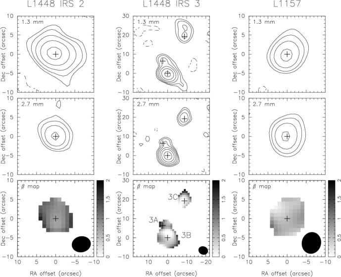
Figure 1.— Dust continuum in $\lambda=1.3$ mm and $2.7$ mm and dust opacity spectral index ($\beta$) maps of L1448 IRS 2, L1448 IRS 3, and L1157. Note that most $\beta$ values are less than 1. The gray scales are the same in all three maps, although the values are distributed in different ranges. The statistics of the values are in Tab. 3. Synthesized beams are the same in all three maps towards each target (Tab. 2) and plotted on the bottom right of the $\beta$ maps. The L1448 IRS 3A, 3B, and 3C positions came from Looney et al. (2000) and the $\lambda=1.3$ mm map of L1448 IRS 3 was re-centered; the pointing center was $\textrm{(RA, Dec)}\approx(-4\arcsec,8\arcsec)$. The contours of dust continuum maps are 3, 5, 9, 17, 33, and 65 times $\sigma=3.4$ and 1.1 mJy beam^-1 ($\lambda=1.3$ mm and 2.7 mm maps of L1448 IRS 2), 10 and 1.6 mJy beam^-1 ($\lambda=1.3$ mm and 2.7 mm maps of L1448 IRS 3), and 13 and 2.4 mJy beam^-1 ($\lambda=1.3$ mm and 2.7 mm maps of L1157).

Figure 2.— Amplitude (upper panels) and dust opacity spectral index $\beta$ plots (lower panels) of the three targets, L1448 IRS 2, L1448 IRS 3B, and L1157, along uv distance. The open squares present $\lambda=1.3$ mm data and the open triangles are for $\lambda=2.7$ mm data. The error bars in the amplitude plots are statistical standard errors of visibilities in each bin. The solid and dashed lines present the best fit models described in § 5 and Fig. 3. The open circles and error bars with caps in the $\beta$ plots indicate $\beta$ values and distribution regions corresponding to the amplitude statistical errors. The filled circles and error bars without caps present cases assuming 15% higher amplitudes at $\lambda=1.3$ mm and 10% lower amplitudes at $\lambda=2.7$ mm (resulting in the largest $\beta$ case within absolute flux calibration uncertainty) and 15% lower at $\lambda=1.3$ mm and 10% higher at $\lambda=2.7$ mm (resulting in the smallest $\beta$ case). The $\beta$ values are calculated at the uv distance bin centers of the $\lambda=1.3$ mm data. The visibilities of $\lambda=2.7$ mm at the positions are interpolated linearly using nearest bin values and in the case of extrapolation the nearest bin values are assumed. The solid line in the $\beta$ plot of L1448 IRS 3B is a logarithmic fit to the data. Refer to the text for further details.

Figure 3.— Model fitting results of three Class 0 sources in likelihood. The contour levels are from 90% of the peak value with steps of 10%. The triangles mark best fit $p$ and $\beta$ pairs and circles indicate likelihood weighted averages of $p$ and $\beta$. To indicate that the model of L1448 IRS 3B is not the most reliable one in this paper (refer to § 6), its contours are presented by dashed lines. The two dotted contours of L1157 indicate 90% and 80% of the peak likelihood based on all models in the parameter ranges of Tab. 4 and the solid contours are the likelihood distribution obtained from better limited models. Refer to the text for details. In the two cases, the best fit model is identical and the likelihood weighted averages are slightly different.

Figure 4.— Likelihood plots of two cases, (a) dashed contours: model of a black body (optically thick) central point source same in Fig. 3 and (b) dotted contours: model of a central point source with a $\beta$ same as the envelope. Triangles presents best fit values and circles indicate likelihood weighted average values. Note that the best model of case (b) gives a worse fit ($\chi_{\nu}^{2}\sim 11$) than case (a) ($\chi_{\nu}^{2}\sim 8.7$). The contour levels are 80%, 60%, and 40% of each likelihood peak value.

Figure 5.— Examples of fitting models to emphasize a radial dependence of $\beta$. The solid lines are the best fit model with $\beta$ as a function of radius ($\chi_{\nu}^{2}\sim 7.1$) and the dotted lines present an example of fitting models with a constant $\beta$. Parameter sets for the best fit model (solid line): $p=2.6$, $M_{T}=2.20$ M_⊙, $\beta_{out}=1.7$, $R_{\beta}=400$ AU, $R_{in}=10$ AU, $R_{out}=4500$ AU, $F_{pt}=0.0$ Jy, $T_{0}=100$ K at $R_{0}=10$ AU and for the other one of a constant $\beta$ (dotted line): $p=2.5$, $M_{T}=2.80$ M_⊙, $\beta=1.0$, $R_{in}=10$ AU, $R_{out}=4500$ AU, $F_{pt}=0.0$ Jy, $T_{0}=100$ K at $R_{0}=10$ AU. Note that the data points are the same as in Fig. 2 and the error bars are statistical standard errors. No absolute flux calibration uncertainties are shown.

Figure 6.— Likelihood plot for models with variable $\beta$ along the envelope radius. $R_{\beta}$ is the radius where $\beta=1.7$ outward. Refer to the text for detailed discussions.

References

- Adams (1991) Adams, F. C. 1991, ApJ, 382, 544
- Andre et al. (1993) Andre, P., Ward-Thompson, D., & Barsony, M. 1993, ApJ, 406, 122
- Andrews & Williams (2005) Andrews, S. M. & Williams, J. P. 2005, ApJ, 631, 1134
- Andrews & Williams (2007) —. 2007, ApJ, 659, 705
- Bachiller & Cernicharo (1986) Bachiller, R. & Cernicharo, J. 1986, A&A, 168, 262
- Bachiller et al. (2001) Bachiller, R., Pérez Gutiérrez, M., Kumar, M. S. N., & Tafalla, M. 2001, A&A, 372, 899
- Beckwith & Sargent (1991) Beckwith, S. V. W. & Sargent, A. I. 1991, ApJ, 381, 250
- Beckwith et al. (1990) Beckwith, S. V. W., Sargent, A. I., Chini, R. S., & Guesten, R. 1990, AJ, 99, 924
- Beltrán et al. (2004) Beltrán, M. T., Gueth, F., Guilloteau, S., & Dutrey, A. 2004, A&A, 416, 631
- Blum (2000) Blum, J. 2000, Space Science Reviews, 92, 265
- Briggs (1995) Briggs, D. S. 1995, PhD thesis, New Mexico Institute of Mining and Technology
- Chandler & Richer (2000) Chandler, C. J. & Richer, J. S. 2000, ApJ, 530, 851
- Chiang et al. (2008) Chiang, H.-F., Looney, L. W., Tassis, K., Mundy, L. G., & Mouschovias, T. C. 2008, ApJ, 680, 474
- Chokshi et al. (1993) Chokshi, A., Tielens, A. G. G. M., & Hollenbach, D. 1993, ApJ, 407, 806
- Ciolek & Mouschovias (1996) Ciolek, G. E. & Mouschovias, T. C. 1996, ApJ, 468, 749
- Curiel et al. (1990) Curiel, S., Raymond, J. C., Moran, J. M., Rodriguez, L. F., & Canto, J. 1990, ApJ, 365, L85
- Draine (1985) Draine, B. T. 1985, in Protostars and Planets II, ed. D. C. Black & M. S. Matthews, 621–640
- Draine (2006) Draine, B. T. 2006, ApJ, 636, 1114
- Finkbeiner et al. (1999) Finkbeiner, D. P., Davis, M., & Schlegel, D. J. 1999, ApJ, 524, 867
- Flower et al. (2005) Flower, D. R., Pineau Des Forêts, G., & Walmsley, C. M. 2005, A&A, 436, 933
- Gueth et al. (2003) Gueth, F., Bachiller, R., & Tafalla, M. 2003, A&A, 401, L5
- Harvey et al. (2003) Harvey, D. W. A., Wilner, D. J., Myers, P. C., Tafalla, M., & Mardones, D. 2003, ApJ, 583, 809
- Hildebrand (1983) Hildebrand, R. H. 1983, QJRAS, 24, 267
- Hogerheijde & Sandell (2000) Hogerheijde, M. R. & Sandell, G. 2000, ApJ, 534, 880
- Kwon et al. (2006) Kwon, W., Looney, L. W., Crutcher, R. M., & Kirk, J. M. 2006, ApJ, 653, 1358
- Kwon et al. (2009) Kwon, W., Looney, L. W., & Mundy, L. G. 2009, in preparation
- Li & Draine (2001) Li, A. & Draine, B. T. 2001, ApJ, 554, 778
- Looney et al. (2000) Looney, L. W., Mundy, L. G., & Welch, W. J. 2000, ApJ, 529, 477
- Looney et al. (2003) —. 2003, ApJ, 592, 255
- Looney et al. (2007) Looney, L. W., Tobin, J. J., & Kwon, W. 2007, ApJ, 670, L131
- Mouschovias (1991) Mouschovias, T. C. 1991, ApJ, 373, 169
- Natta et al. (2007) Natta, A., Testi, L., Calvet, N., Henning, T., Waters, R., & Wilner, D. 2007, in Protostars and Planets V, ed. B. Reipurth, D. Jewitt, & K. Keil, 767–781
- O’Linger et al. (1999) O’Linger, J., Wolf-Chase, G., Barsony, M., & Ward-Thompson, D. 1999, ApJ, 515, 696
- Ossenkopf & Henning (1994) Ossenkopf, V. & Henning, T. 1994, A&A, 291, 943
- Pollack et al. (1994) Pollack, J. B., Hollenbach, D., Beckwith, S., Simonelli, D. P., Roush, T., & Fong, W. 1994, ApJ, 421, 615
- Poppe et al. (2000) Poppe, T., Blum, J., & Henning, T. 2000, ApJ, 533, 454
- Sault et al. (1995) Sault, R. J., Teuben, P. J., & Wright, M. C. H. 1995, in Astronomical Society of the Pacific Conference Series, Vol. 77, Astronomical Data Analysis Software and Systems IV, ed. R. A. Shaw, H. E. Payne, & J. J. E. Hayes, 433–+
- Seale & Looney (2008) Seale, J. P. & Looney, L. W. 2008, ApJ, 675, 427
- Shirley et al. (2000) Shirley, Y. L., Evans, II, N. J., Rawlings, J. M. C., & Gregersen, E. M. 2000, ApJS, 131, 249
- Shu (1977) Shu, F. H. 1977, ApJ, 214, 488
- Spitzer (1978) Spitzer, L. 1978, Physical processes in the interstellar medium (New York Wiley-Interscience, 1978. 333 p.)
- Tassis & Mouschovias (2005) Tassis, K. & Mouschovias, T. C. 2005, ApJ, 618, 783
- Terebey & Padgett (1997) Terebey, S. & Padgett, D. L. 1997, in IAU Symp. 182: Herbig-Haro Flows and the Birth of Stars, 507–514
- Thompson et al. (2001) Thompson, A. R., Moran, J. M., & Swenson, Jr., G. W. 2001, Interferometry and Synthesis in Radio Astronomy, 2nd Edition (Interferometry and synthesis in radio astronomy by A. Richard Thompson, James M. Moran, and George W. Swenson, Jr. 2nd ed. New York : Wiley, c2001.xxiii, 692 p. : ill. ; 25 cm. ”A Wiley-Interscience publication.” Includes bibliographical references and indexes. ISBN : 0471254924)
- Tobin et al. (2007) Tobin, J. J., Looney, L. W., Mundy, L. G., Kwon, W., & Hamidouche, M. 2007, ApJ, 659, 1404
- Visser et al. (1998) Visser, A. E., Richer, J. S., Chandler, C. J., & Padman, R. 1998, MNRAS, 301, 585
- Wolfire & Cassinelli (1986) Wolfire, M. G. & Cassinelli, J. P. 1986, ApJ, 310, 207
- Woody et al. (2004) Woody, D. P., Beasley, A. J., Bolatto, A. D., Carlstrom, J. E., Harris, A., Hawkins, D. W., Lamb, J., Looney, L., Mundy, L. G., Plambeck, R. L., Scott, S., & Wright, M. 2004, in Presented at the Society of Photo-Optical Instrumentation Engineers (SPIE) Conference, Vol. 5498, Millimeter and Submillimeter Detectors for Astronomy II. Edited by Jonas Zmuidzinas, Wayne S. Holland and Stafford Withington Proceedings of the SPIE, Volume 5498, pp. 30-41 (2004)., ed. C. M. Bradford, P. A. R. Ade, J. E. Aguirre, J. J. Bock, M. Dragovan, L. Duband, L. Earle, J. Glenn, H. Matsuhara, B. J. Naylor, H. T. Nguyen, M. Yun, & J. Zmuidzinas, 30–41
- Yan et al. (2004) Yan, H., Lazarian, A., & Draine, B. T. 2004, ApJ, 616, 895