ON MEASURING ACCURATE 21 CM LINE PROFILES WITH THE ROBERT C. BYRD GREEN BANK TELESCOPE

Abstract

We use observational data to show that 21 cm line profiles measured with the Green Bank Telescope (GBT) are subject to significant inaccuracy. These include $\sim$10% errors in the calibrated gain and significant contribution from distant sidelobes. In addition, there are $\sim$60% variations between the GBT and Leiden/Argentine/Bonn 21 cm line profile intensities, which probably occur because of the high main-beam efficiency of the GBT. Stokes $V$ profiles from the GBT contain inaccuracies that are related to the distant sidelobes.

We illustrate these problems, define physically motivated components for the sidelobes, and provide numerical results showing the inaccuracies. We provide a correction scheme for Stokes $I$ 21 cm line profiles that is fairly successful and provide some rule-of-thumb comments concerning the accuracy of Stokes $V$ profiles.

1 INTRODUCTION

The Robert C. Byrd Green Bank Telescope (GBT) has no aperture blockage from mechanical structures such as feed legs. In conventional telescopes, scattering from such structures produces distant sidelobes far from the main beam, which are particularly important in contaminating 21 cm line profiles with “stray radiation”. For example, when observing a weak high-latitude position with a sidelobe lying on the Galactic plane, the profile can be heavily contaminated. The nature of the contamination depends both on hour angle, because the distant sidelobes might hit the ground instead of the sky, and on the observing epoch, because of Doppler shifts from the Earth’s orbital motion. A great advance in 21 cm line survey data occurred when Kalberla et al. (2005) corrected both northern and southern sky 21 cm line survey data for stray radiation; the resulting “LAB” (Leiden/Argentine/Bonn) survey is largely free of stray radiation.

With its absence of aperture blockage, one would expect the GBT to have very low stray radiation. However, this is not the case, as first shown by Lockman & Condon (2005). We have used the GBT to measure Zeeman splitting of the 21 cm line, which requires long integrations. For four circumpolar positions we have nearly full 24-hour coverage. We observe systematic time variations during the observing periods, both in Stokes $I$ and Stokes $V$. These are reminiscent of stray radiation. The present paper explores these effects for both Stokes $I$ and $V$ observations, and for Stokes $I$ presents an approximate correction scheme to remove these contaminants.

We begin in §2 by describing the basic properties of the GBT primary beam in both Stokes $I$ and $V$. However, the telescope’s response is not limited to just the primary beam: §3 shows the contribution of stray radiation to the time variability of Stokes $I$ and $V$ 21 cm line profiles at the North Celestial Pole (NCP). §4 presents observations of the Sun, far from the main beam, which show distant sidelobes related to spillover from the secondary reflector. This section defines three sidelobe components motivated by structural and physical considerations: the spillover, the spot, and the screen components. §5 uses observations of Cas A to define the fourth (“nearin”) component, which is related to the diffraction rings of the primary beam. §6 outlines the least-squares procedure that we used to solve for the amplitude coefficients of the four components and §7 presents the results of the least-squares analysis for full hour-angle coverage of four positions; these results include not only the amplitude coefficients, but also the errors in calibrated system gains and the true profile of the observed position. In particular, §7.3 shows the contributions of the four components and how they change with time for the four sources, and shows how well their sum—which is the total predicted spillover profile—predicts the actual time behavior.

The first sections, summarized above, focus on Stokes $I$. §8 treats Stokes $V$ 21 cm line profiles. This is necessarily less detailed than the Stokes $I$ discussion, because the sidelobe structures for Stokes $V$ are much more complicated, as shown by our observations of the Sun and Cas A. We find that the primary contributor to stray radiation in Stokes $V$ is the screen component, which lies close to the main beam and has very complicated structure. Without considerable effort, which would involve high dynamic-range observations of this component in Stokes $V$, it is impossible to correct observed profiles. Rather, we discuss the Stokes $V$ contamination as a fraction of the screen’s Stokes $I$ predicted profile and propose a rule of thumb for the reliability of Stokes $V$ 21 cm line profiles measured with the GBT.

2 BASIC PROPERTIES OF THE GBT PRIMARY BEAM AT 1420 MHZ

For all observations in this paper, we used the GBT and the Spectral Processor backend (Fisher, 1991). All data were analyzed using algorithms written by the authors in the Interactive Data Language (IDL).

We used 3C 286 as a polarization calibrator on a number of different occasions from 2003 January to 2006 July, observing the eight-legged star-shaped pattern of Heiles et al. (2001). In the range 1–2 GHz, we observed at four frequencies simultaneously: {1160, 1420, 1666, 1790} MHz. These observations provided the beam parameters. Heiles et al. (2003) reported on the results of these observations; however, their analysis was flawed because of a computer program error by one of us (CH), so we present updated values here. We find:

1. At 1420 MHz, the primary beam full width at half maximum (FWHM) is $9.088\pm 0.009$ arcmin. The beamwidth is proportional to wavelength to within $1.7\%$ (rms) among the four frequencies.

2. The fractional main beam ellipticity, defined as

   $$fractional\ beam\ ellipticity=\frac{{\rm FWHM}_{\rm max}-{\rm FWHM}_{\rm min}}{{\rm FWHM}_{\rm max}+{\rm FWHM}_{\rm min}}\ ,$$ (1)

   is less than $1\%$ and mostly less than $0.5\%$.

3. The beam squint in Stokes $V$ changes systematically with zenith angle, ZA, and it also changes with frequency. Figure 1 exhibits this behavior for two frequencies of interest, the 21 cm line and the 18 cm OH lines. We define beam squint as the difference in central position of the two circularly polarized beams.

   

   Figure 1: Stokes $V$ Beam Squint versus zenith angle for 1420 and 1666 MHz.

4. The beam squash in Stokes $V$ is about 1$\arcsec$ and changes little, if at all, with ZA. It changes little among our three lowest frequencies, but triples for the highest frequency (1790 MHz). Figure 2 exhibits the squash behavior for two frequencies of interest, the 21 cm line and the 18 cm OH lines. We define beam squash as the difference between the FWHM in the orthogonal circular polarizations. Beam squash samples the second angular derivative of the sky brightness, and a FWHM difference of order 1$\arcsec$ produces essentially no detectable effect unless the sky brightness changes extremely rapidly with position.

   

   Figure 2: Stokes $V$ Beam Squash versus zenith angle for 1420 and 1666 MHz.

3 EMPIRICAL EVIDENCE FOR STRAY RADIATION: TIME-DEPENDENT STOKES $I$ AND $V$ 21 CM LINE PROFILES

Figure 3: Changes with time of the GBT 21 cm line profile for the North Celestial Pole (NCP) observed in 2003 September, with Stokes $I$ on the left and Stokes $V$ on the right. Each panel shows averages over 4 hours of LST. For Stokes $I$, the solid-line profiles are differences between the 4-hour average and the 24-hour average. The dotted profile is the scaled-down 24-hour average Stokes $I$ profile; its left and right peaks have 20 and 50 K, respectively, as indicated. For Stokes $V$, the solid-line profiles are the observed ones and the dashed is the 24-hour average.

Figure 3 depicts the time variability of the GBT Stokes $I$ and $V$ 21 cm line profiles for observations of the North Celestial Pole (NCP). For Stokes $I$, shown in the left panels, the data are averaged in 4-hour bins and the 24-hour average is subtracted. Differences typically amount to $\sim$1 K For the peaks, amounting to a fractional change of a few percent. More serious, however, at $-$40 km s^-1 the mean profile has temperature $\sim$3 K and the fractional change is $\sim$30%. The profile distortions sometimes change rapidly with time. For example, the $-$40 km s^-1 intensity peaks sharply in the LST = 0–4 hr bin.

For Stokes $V$, shown in the right panels, the data are averaged in 4-hour bins and shown as solid lines; the 24-hour average is shown as dashed. Changes are clearly obvious. Most extreme are the ${\rm LST}=6\pm 2$ hr bin, where the signal almost disappears, and the ${\rm LST}=18\pm 2$ hr bin, where there is a broad positive bump centered near $-$25 km s^-1. Other bins also show shape changes.

4 SIDELOBES RELATED TO THE SECONDARY REFLECTOR

4.1 Descriptive Discussion

Figure 4 exhibits Stokes $I$ versus AZ/ZA great-circle offset coordinates for four scans through the Sun taken on 2003 September 19; data on 2003 September 7 are essentially identical, so all features are real. The right panel shows the four scans with azimuthal width proportional to the observed intensity. The dashed circle shows the approximate boundary of the secondary reflector as seen by the feed (the actual boundary is slightly elliptical; see Figure 5). The left panel shows the intensity profiles versus great-circle angular offset from the main beam.

Figure 4: Four Stokes $I$ scans (“Legs”) through the Sun in AZ/ZA great-circle offset coordinates. In the left panel we plot the measured antenna temperatures versus the angular offsets from the main beam center. In the right panel, the azimuthal thicknesses of the lines are proportional to the measured temperatures; the dashed circle represents the approximate boundary of the secondary reflector as seen by the feed. The begin and end points of the legs are labelled on each panel by “,0” and “,1”, respectively. On the left panel, the arrows lie $5^{\circ}$ outside the dashed circle. On both panels, the spot marks the Arago spot.

Figure 4 shows that there is significant response outside of the main beam. We represent this response by three components, which are motivated by applying intuitive physical considerations to the reflector geometries given by Norrod & Srikanth (1996):

1. The Spillover ring. Leg 0 and the lower halves of Legs 1, 2, and 3 reveal the spillover contribution from the secondary, which peaks about $5^{\circ}$ outside of the dashed circle. The term “spillover” refers to radiation transmitted from the feed toward the secondary reflector that would “spill over” its edge. Clearly, the spillover is not simply what we would find from geometrical optics, which would have a sharp cutoff located at the reflector edge. Rather, the profiles show diffraction effects, with the peak lying outside the occulting edge and a gradual decrease in intensity toward the inside of the occulting area, as predicted by physical optics (Kraus, 1988). Arrows on the left panel of Figure 4 mark $5^{\circ}$ outside the reflector edge, roughly at the peak except for Leg 0. The decrease outside the peak is caused by the taper of the feed’s illumination of the secondary.

   We represent this spillover pattern as being circularly symmetric about the axis of the subreflector center. However, careful inspection of Figure 4 reveals that this symmetrical condition does not, in fact, obtain. Comparing the peak locations with the arrows, which are located $5^{\circ}$ outside the subreflector edge, it is clear that the radial distance of the peaks of Leg 0 is larger than the radial distances of the other peaks. A degree of noncircularity is expected because the secondary, as seen from the feed, is slightly elliptical; see Figure 5. From this figure, we see that the secondary is slightly narrower in the AZ direction. Because Leg 0 samples the AZ direction more than the ZA direction, the narrower ellipse projection suggests that the peaks along Leg 0 should lie closer, not further, than the other scans’ peaks, opposite to what we see. We attribute this apparent turnabout to structural components that lie behind the secondary and protrude out from its projected edge, which are apparent as the “ears” in Figure 5; Leg 0 passes close to these ears.

2. The Arago spot. A striking feature on Leg 2 is a small, intense spot, marked with a black spot. This is the famous Arago spot of an occulting disk. According to Sommerfeld (1954), the intensity of the Arago spot for incoming parallel plane waves should be equal to the peak intensity of radiation near the edge of the blockage. Figure 4 shows that this condition is achieved quite closely. We measure the Arago spot to be centered $0.39^{\circ}$ below the subreflector center (i.e., toward the primary beam); this offset occurs because the axis of the secondary is tilted with respect to the line joining the feed and subreflector center.

3. The Screen component. Figure 4 shows that there is excess intensity near the main beam, which we call the “screen” component. Careful examination of Figure 4 shows that this excess tends to be asymmetric about the main beam center, with excess intensities tending toward negative ZA offsets. This is particularly apparent when comparing the lower half of Leg 2 with those of Legs 1 and 3, and also with the nearby structure of Leg 0. It seems like a separate beam a few degrees in size that is offset from the main beam center by a few degrees.

   In our mind’s eye, we attribute this to the reflecting “screen,” which controls the spillover radiation that hits the structural components of the feed arm. At the top of Figure 5 we see these feed-arm structural components. This jumble of metal beams would uncontrollably scatter the spillover radiation. To control this component, the telescope engineers installed a flat reflecting screen on the feed arm near the subreflector (Norrod, 1990). This screen directs radiation coming from the feed back to the primary reflector, and then to cold sky. It is as if a separate source of radiation centered on the screen illuminates the primary reflector; this source, the screen, is located near the intersection of Leg 2 with the dashed circle at the top of Figure 5, at positive ZA offset with respect to the subreflector. Being offset toward positive ZA offset, upon reflection from the primary reflector it would point toward negative ZA offset. We think that this might be responsible for the excess asymmetric intensity and this is why we call this the “screen” component.

   Radiation that is removed from the spillover by the screen, which we discussed in the above paragraph, eliminates radiation from an angular slice of the spillover pattern. We don’t know how big this slice is, so we incorporated it as an unknown in our least-squares fits described below in §6.

Figure 5: The GBT secondary as seen from the feed, oriented so that the feed leg is on top—the same orientation as in Figure 4. The secondary looks slightly elliptical, with the major axis in the vertical (ZA) direction. Image courtesy of NRAO/AUI.

4.2 Caveat

Our characterization of the GBT sidelobe structure is necessarily approximate because we have limited mapping data in Figure 4. Our characterization is based on this sparse sampling together with physical reasoning and intuition. The quantitative representation that we present below should be regarded as a convenient approximation meant for the purposes of correcting 21 cm line data, not as an accurate description of the sidelobes.

4.3 Quantitative Representation

In the equations below, the intensity scale is parameterized by the multiplying coefficient $H$. The units of $H$ are left undefined. Rather, as explained in §6.2, we normalize the area of each component’s beam to unity so that its integrated response over the sky is in units of the main beam’s integrated response. For the three components, we have:

1. The Spillover ring. We represent the spillover ring by a sum of two two-dimensional Gaussian rings. The response $P_{\rm ring}(\theta)$ of each Gaussian ring is characterized by a radial distance $\theta_{\rm ring}$ of its peak from the center of the subreflector, an angular half-power full width FWHM, and a height $H$. That is, each ring has the functional form

   $$P_{\rm ring}(\theta)=H_{\rm ring}\exp\left[-\frac{\left(\theta-\theta_{\rm ring}\right)^{2}}{2({\rm FWHM}/2.35)^{2}}\right]\,,$$ (2)

   where $\theta$ is the angular distance from the subreflector center. The parameters for the two Gaussians are: $H_{\rm ring}=[1.14,1.0]$ (arbitrary units); $\theta_{\rm ring}=[20.6^{\circ},16.4^{\circ}]$; ${\rm FWHM}=[3.3^{\circ},8.8^{\circ}]$. To account for the radiation scattered by the screen, we remove an angular slice of total width $49^{\circ}$ centered on the feed leg—centered opposite the main beam as seen from the subreflector center.

2. The Arago Spot. We represent the response of the Arago spot $P_{\rm spot}$ by a two-dimensional Gaussian spot whose center is offset $0.39^{\circ}$ toward the main beam from the subreflector center; its FWHM is $1.09^{\circ}$. The functional form is

   $$P_{\rm spot}(\Delta{\rm AZ},\Delta{\rm ZA})=H_{\rm spot}\exp\left[-\frac{\Delta{\rm AZ}^{2}+(\Delta{\rm ZA}+0.39)^{2}}{2({\rm FWHM}/2.35)^{2}}\right]\,,$$ (3)

   where $(\Delta{\rm AZ},\Delta{\rm ZA})$ are measured in degrees from the center of the subreflector as seen by the feed.

3. The Screen component. We represent the screen response as a two-dimensional Gaussian ring with ${\rm FWHM}=0.5^{\circ}$ and radial offset from main beam center $\theta_{\rm screen}=2.8^{\circ}$. The amplitude of the Gaussian depends on $\phi$, the azimuthal angle around main beam center in $(\Delta{\rm AZ},\Delta{\rm ZA})$ space. The functional form is

   $$P_{\rm screen}(\theta,\phi)=H_{\rm screen}(\phi)\exp\left[-\frac{\left(\theta-\theta_{\rm screen}\right)^{2}}{2({\rm FWHM}/2.35)^{2}}\right]\,,$$ (4)

   where $\theta$ is the angular distance from main beam center and $\phi=\arctan(\Delta{\rm AZ}/\Delta{\rm ZA})$, measured counterclockwise from the $-\Delta{\rm ZA}$ axis. We estimated the amplitude $H_{\rm screen}(\phi)$ from the Sun scan legs seen in Figure 4: we forced an 8-term Fourier representation, which is shown in Figure 6 and is clearly a crude approximation.

Figure 6: $H_{\rm screen}(\phi)$ of equation (4) versus $\phi$.

4.4 Pictorial Representation

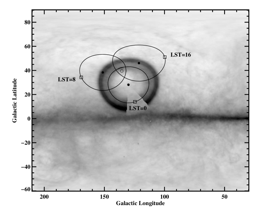
Figure 7: Images of the secondary-reflector sidelobes at three LSTs for the position G135.5$+$39.5, superposed on the integrated 21 cm line intensity from the LAB survey. The empty circle is the source position. The filled circles are the Arago spot. The solid $30^{\circ}$-diameter circles approximately show the subreflector edge as seen by the feed. Each of the three squares lies on its subreflector circle just inside the feed arm. The circular grayscale image has darkness proportional to the spillover pattern; this is shown only for LST=0. The blanked-out portion of the spillover pattern is the angular slice of the screen.

The discussion and equations of §4.1 and §4.3 represent an attempt to mathematically approximate the contributions of the expected sidelobe response of the GBT. We can gain an understanding of these sidelobes by mapping them on the sky. Figure 7 shows the spillover lobe, its screen slice, and the Arago spot when observing the position G135.5$+$39.5 at LST = 0, 8, and 16 hr. These are all evaluated for the adopted parameter values given in §7.

The spillover lobe intensity is shown by the large, circular grayscale ring. It peaks about $5^{\circ}$ outside of the subreflector edge, which is shown as a $30^{\circ}$-diameter circle. The Arago spot lies about halfway between the main beam (empty circle) and the feed arm (which lies just outside the square). We don’t show the screen component on Figure 7, because it lies close to the main beam—$2.8^{\circ}$ away, on the opposite side of the main beam (i.e., the source position) from the Arago spot.

At LSTs near 1 hr, the spillover lobe brushes the Galactic plane; with the large velocities of Galactic rotation, this produces significant contributions to the observed profile at intermediate and high velocities. 12 hours later the spillover lies far from the Galactic plane and there is no measurable contribution.

5 THE STOKES $I$ DIFFRACTION RINGS OF THE PRIMARY BEAM

5.1 Descriptive Discussion

Figure 8 represents the GBT diffraction rings as probed by scans through Cas A. The results are shown in two ways, with intensity versus position offset for four observed legs in the left panel and a map in the right. The first ring is not circularly symmetric about beam center. Rather, it is strongest at positive ZA offset and weakest at negative offset. This is clear from examining Leg 2 on the left panel, whose first ring peak at positive offset exceeds 10 K and at negative offset is obviously less. In other words, the rings’ responses depend on $\phi$ [here, $\phi=\arctan(\Delta{\rm ZA}/\Delta{\rm AZ})$]. In contrast, the $\phi$ asymmetry for the second ring looks opposite to that of the first. Clearly, the situation regarding asymmetry in $\phi$ is complicated and cannot be easily described analytically. We use an oversimplified quantitative model for the diffraction rings because their structure is complicated and we do not have complete and accurate data.

Figure 8: Four Stokes $I$ scans (“Legs”; displaced zeros) through Cas A in AZ/ZA great-circle offset coordinates, showing the first three diffraction rings. In the left panel we plot the measured antenna temperatures versus the angular offsets from the main beam center. In the right panel, the azimuthal thicknesses of the lines are proportional to the measured temperatures. The begin and end points of the legs are labelled on each panel by “,0” and “,1”, respectively. On the left, dotted lines show intensity offsets of 5 and 10 K for each leg.

We split the diffraction rings into two parts: (1) the average over $\phi$ and (2) the portion that changes with $\phi$. (If we were to represent the $\phi$ behavior with a Fourier series, the first would be the “DC” term):

1. For the $\phi$-averaged part, the 21 cm line profile contribution is independent of parallactic angle PA (i.e., hour angle). This contribution is small. The peak amplitude of the first ring is about 1000 times weaker than the peak of the main beam. The angular areas of the rings exceed those of the main beam. With these, the net angle-integrated beam response of the rings is no more than $\sim$1% of the main beam’s. Because the rings lie close to the main beam, the spectral shape of their contribution is similar to that of the main beam’s, so they simply augment the main beam’s profile by a small amount. Our analysis lumps these together, so that elsewhere in this paper when we use language such as the “integrated response of the main beam,” we in fact mean the contribution of the main beam plus the $\phi$-averaged response of the diffraction rings.

2. For the $\phi$-variable portion, we adopt a very simple model. We assume (1) that the $\phi$ dependence is independent of radial offset from beam center, and (2) that the $\phi$ dependence is described by the lowest Fourier mode [i.e., $\propto\cos(\phi-\phi_{0})$]. The first assumption is clearly invalid, given our discussion of Figure 8 in the above paragraph, but as we mentioned, the situation is complicated. We expect our oversimplified ring treatment to produce inaccuracies in our predicted spectra.

5.2 The “Nearin” Component

With our assumptions, we can represent the $\phi$-variable portion by the difference between two primary beams pointing on opposite sides of beam center. We name this the “Nearin” component. We don’t use the name “Ring,” because this representation is only an approximation. To determine the appropriate parameters, we assumed the position difference between the beams to be 5 arcmin and performed the least-squares procedure of §6 for a grid of $\phi_{s}$ values, where $\phi_{s}$ is the angle of the position difference; we obtained $\phi_{s}=180^{\circ}$. (If the first ring alone were responsible, the left panel of Figure 8 shows that we would have obtained $\phi_{s}=90^{\circ}$.)

The other three sidelobe contributions have nonzero (positive) sky-integrated beam responses. However, the sky-integrated response of the Nearin component is zero, because it is the difference between two main beam pointings. In particular, the profile predicted from this component can be both positive and negative. Thus, our discussion below about the physical meaning of the derived $\alpha$ coefficients in §6.2 applies to the other three sidelobe contributions, but not to the Nearin one.

6 DERIVING THE STOKES $I$ SIDELOBE AMPLITUDES USING 21 CM LINE DATA AND THE METHOD OF LEAST SQUARES

6.1 The General Approach

While our Sun scans of §4 allow us to measure the sidelobe beam shapes with fair accuracy, we cannot measure the amplitudes. The peak response of these sidelobes is more than $\sim$1000 times smaller than the peak on-axis beam response (for the diffraction rings) and at least another 10 times smaller for the spillover and spot beams. The linear dynamic range of modern radioastronomical receiving systems is limited by both analog and digital electronics and the net response is highly nonlinear over such large ranges. Therefore, rather than try to correct for saturation effects by bootstrap calibration techniques or to rely on theoretical calculations, we use observations of the 21 cm line at four positions to define the approximate contaminating beam shapes and use least-squares fitting to obtain their amplitudes. We present our technique below, but first we mention a set of details that should be kept in mind.

6.2 Four Important Details

There are four important details that should be considered concerning these fits:

1. The spillover and spot cover areas of sky located at considerable angular distances from the observed position. Doppler corrections differ substantially over these angular distances. The LAB survey provides profiles in the Local Standard of Rest (LSR) system; given that we observe in the topocentric reference frame, we must convert all LAB profiles to topocentric velocities. Upon obtaining the estimated sidelobe response, the spectrum must be converted back to the LSR reference frame for the position actually pointed at.

   Table 1: LAB/GBT Intensity Ratios

   Source Name	(LAB/GBT)
   G139.1$+$0.7	0.845
   W3off (G133.8$+$0.8)	0.804
   G135.5$+$39.5	1.409
   NCP (G122.9$+$27.1)	1.275

2. For each of the four positions, the several hundred spectra included in each fit were obtained over at least a 24-hour interval and often over several days. We find that the gains are not perfectly calibrated. That is, even though the spectral shapes are unaffected, the calibrated intensity scales change with time as these gains change. We need to assign each observed spectrum its own gain and include the set of gains as unknowns in the fit.

3. The overall intensity scale of the GBT spectra, relative to that of the LAB spectra, changes from one position to another as shown in Table 1. The ratio of LAB to GBT intensities (LAB/GBT) ranges from 0.80 to 1.41, changing by a factor of 1.75, with smaller values associated with sources in the Galactic plane and larger values associated with high-latitude positions. These numbers are obtained from the least-squares fits for $G_{s}^{*}$ in equation (5), so they are not a result of sidelobe contributions.

   The sense of this—higher ratios in the Galactic plane—is contrary to what we’d expect from the angular structure of the H I line. In the Galactic plane, the H I line intensity has a relatively small fractional variation over the scale of 40 arcminutes, so the H I emission fills the main beams of both the GBT and the LAB telescopes. In contrast, for the two high-latitude positions, the H I structure is filamentary with widths of order $\leq$10 arcmin, as shown by 100 $\mu$m IRAS maps (Jackson et al., 2003) and, also, our currently unpublished GBT 21 cm maps of this area. The GBT main beam is filled, or nearly filled, by the H I emission; but the larger beams of the LAB telescopes are not filled—nor are their nearin diffraction lobes. So we expect lower LAB/GBT ratios for the high-latitude positions, contrary to the numbers in Table 1.

   We suspect that the suggested trend in Table 1 for higher ratios at the high-latitude positions is an illusionary result of small-number statistics. We specifically do not believe that varying ratios of LAB/GBT are produced by problems with the LAB spectra, because great care has been taken to ensure their accuracy and, also, they have been carefully corrected for sidelobe problems. Therefore, we conclude that the intensity scale of the GBT H I spectra can vary by factors in the above range, namely $\sim\pm 30\%$, for reasons that we cannot fathom.

4. The observed spectrum is contaminated by contributions from the spillover, the Arago spot, the screen, and the Nearin response. The first three of these have nonzero (positive) sky-integrated beam responses, and the Nearin one has zero integrated response. The following discussion applies only to the first three, not to the Nearin component.

   In calculating the beams associated with these three contaminants, we normalize each one so that its gain-area product is unity; we then simultaneously fit for the proper amplitude coefficients (and other quantities; see §6.3), which we call $\alpha$ with appropriate subscripts. With the normalized integrated beam response, $\alpha$ represents the contaminating beam’s integrated “beam efficiency.” That is, if the contaminating beam were placed in a blackbody cavity at temperature $T_{\rm bb}$, it would contribute $\alpha T_{\rm bb}$ to the observed antenna temperature $T_{a}$. Similarly for the main beam, we can define an amplitude coefficient $\alpha_{\rm mb}$, which would equal the classically-defined main-beam efficiency. That is, in the blackbody cavity the main-beam antenna temperature would equal $\alpha_{\rm mb}T_{\rm bb}$.

   We assume that the LAB survey temperature scale is absolutely correct in the sense that the spectral temperatures are, in fact, the actual brightness temperatures. Our least-squares solutions in §6.3 force the GBT temperature scale for the “true spectrum” $T^{*}_{c}$ (see §6.3) to equal the LAB temperature scale. In essence, this is forcing $\alpha_{\rm mb}$ to equal unity. Thus, for one of these first three contaminating beams, its value of $\alpha$ represents its beam efficiency with respect to the main beam efficiency, i.e., $\alpha$ is equal to the contaminating beam’s area-integrated response divided by that of the main beam.

   This is a somewhat awkward situation, because the sum of the four $\alpha$ values exceeds unity. That is, when the GBT is placed in a blackbody cavity of temperature $T_{\rm bb}$, the antenna temperature exceeds $T_{\rm bb}$ by a factor equal to the sum of all four $\alpha$ values. However, if the contaminating beams do not see the walls of the cavity, then the antenna temperature is equal to the brightness temperature. This awkwardness pervades measurements of extended sources by all single dishes, unless the sidelobes and main beam responses are reconciled as they are for the LAB survey (see Hartmann et al. 1996 and Kalberla et al. 2005). The proper reconciliation of these matters is a fundamentally important contribution by the LAB survey. The GBT, with its seeming inability to reliably and self-consistently measure H I line intensities, cannot yet be regarded as a suitable system for obtaining accurately-calibrated H I line profiles.

6.3 The Least-Squares Technique

Suppose we have a number of spectra $S$, each with $C$ spectral channels, taken over a mostly complete range of 24 hours in LST. Let the subscripts $s$ and $c$ denote the spectrum number and spectral channel number, respectively. Let the superscript $o$ designate the observed value and $*$ the true value (which is the same as the noise-free fitted value) that would be observed in the absence of sidelobe contributions and gain errors. Let $T$ denote the intensity, which is normally expressed in units of temperature. As we mentioned in §6.2, the intensity scaling of each spectrum (the “gain” $G_{s}$) is not perfectly calibrated so we solve for the set of spectral gains. As we discussed in §6.2, we normalize each contaminating beam so that its gain-area product is unity; then we fit for the proper scaling parameter, which we call $\alpha$ with an appropriate subscript.

The observed spectrum $T^{o}_{c,s}$ is equal to the true spectrum $T_{c}^{*}$ plus the contaminating contributions from the spillover, the Arago spot, the screen, and the Nearin. We calculate the contaminating spectral contribution of each of the first three by multiplying its beam by appropriately velocity-shifted spectra from the LAB survey. We can use the LAB survey for these beams because their angular scales are large compared to the LAB’s 36-arcmin angular resolution.

However, the Nearin contribution depends on the angular structure close to the GBT main beam, which is on a smaller scale than the LAB survey resolution. For the Nearin contribution, we estimate the angular derivatives of the emission brightness temperature from a 17-point sampling with the GBT centered on the position observed, using the same technique (the “Z16 pattern”: i.e., 16 off-source positions and one on-source) as Heiles & Troland (2003, §2).

The following equation expresses the observed spectrum $T^{o}_{c,s}$ in terms of the true spectrum $T^{*}_{c}$ and the four contaminants $T^{j}_{c,s}$, where the superscript $j$ runs from 0 to 3 and represents spillover, spot, screen, and Nearin, respectively; $j$ also applies to the beams’ $\alpha$ coefficients as a subscript. Note that the contribution from each contaminating spectrum changes with time, so it’s a function of spectrum number $s$.

$$T^{o}_{c,s}=G^{*}_{s}\left[T^{*}_{c}+\sum_{j=0}^{j=3}T^{j}_{c,s}\alpha^{*}_{j}\right]\,.$$ (5)

The total number of equations is $CS$. The unknowns are the starred values: the $S$ values of gain $G_{s}^{*}$, the C values of the true spectral channels $T^{*}_{c}$, and the four $\alpha_{j}^{*}$ values; the total number of unknowns is $(C+S+4)$. We have $CS$ equations, which is many more than the number of unknowns. This is a well-posed least-squares problem.

It is also a nonlinear least-squares problem because the unknown gains $G^{*}_{s}$ multiply the other unknowns. We linearize this equation by Taylor expansion, setting each unknown equal to a “guessed” value with subscript $g$ plus a correction preceded by $\delta$. For example, the true value $T^{*}_{c}=T^{g}_{c}+\delta T_{c}$. In formulating the equations of condition, we treat the guessed values as known, so the corrections become the quantities to solve for. Having solved for the corrections, we apply them to the guessed values and do the fit again, iterating until convergence.

In terms of the guessed and correction values, equation (5) becomes

$$T^{o}_{c,s}=(G^{g}_{s}+\delta G_{s})\left[(T^{g}_{c}+\delta T_{c})+\sum_{j}T^{j}_{c,s}(\alpha^{g}_{j}+\delta\alpha_{j})\right]\,.$$ (6)

The summed quantity $\sum_{j}T^{j}_{c,s}\alpha^{g}_{j}$, which consists of the guessed values for the unknown coefficients, is the guessed value of the observed spectral channel in each iteration, so it is natural to define the correction to the observed value as

$$\delta T^{o}_{c,s}=T^{o}_{c,s}-T^{o,g}_{c,s}\,.$$ (7)

Grouping and retaining only first-order terms, our equations of condition become

$$\delta T^{o}_{c,s}=G^{g}_{s}\ \delta T_{c}+\left[\sum_{j}G^{g}_{s}T^{j}_{c,s}\right]\delta\alpha_{j}+\left[T^{g}_{c}+\sum_{j}T^{j}_{c,s}\alpha^{g}_{j}\right]\delta G_{s}\,.$$ (8)

In these equations (of which there are a total number $CS$), the three $\delta$ quantities represent the $(C+S+4)$ unknowns and all other quantities are either measured or guessed, so are known quantities as far as the fit is concerned.

There is one additional constraint we need to add as a final equation of condition. Consider equation (8). The last term of this equation contains five temperature terms: the first, $T^{g}_{c}$, and the other four, which are the sidelobe contributions $T^{j}_{c,s}\alpha^{g}_{j}$. The first is much larger than the latter four. If we were to add a single constant to all $\delta G_{s}$, and simultaneously scale down $T^{g}_{c}$, the fit would be almost unchanged. Thus, there is a near-degeneracy between these quantities. If we allow this constant to exist, then there is a high negative covariance (a near-degeneracy) between the final values of (1) this constant value added to all $G^{*}_{s}$ and (2) the amplitude scaling of $T^{*}_{c}$. We can remove this covariance—and retain the mean of the original amplitude scaling—by requiring the sum of the guessed gains to remain constant. This is equivalent to requiring

$$\sum_{s=0}^{S-1}\delta G_{s}=0\,.$$ (9)

It is straightforward to form a matrix (the Numerical Recipes “design matrix”; Press et al. 1992, §15.4) from the $CS$ equations 8 and the additional equation (9). We then perform the least-squares solution in the usual way.

6.4 Solving for the Slice Angle

In §6.3 above we do not mention the unknown angle of the slice that is removed by the screen. Nevertheless, we fit for it as an unknown parameter, in addition to the others mentioned above. Instead of incorporating it into the equations of condition, however, we used the “brute-force” technique. That is, we selected a grid of values for the slice angle and carried through the least-squares fit of §6.3 for each assumed value. Then we plotted the variance versus the assumed slice angles. The minimum variance defines the fitted slice angle.

7 LEAST-SQUARES FIT RESULTS FOR THE FOUR SOURCES

7.1 Systematic Changes of Calibrated System Gains

The system gain is obtained by turning on a noise diode, which provides a calibrated broadband noise signal of known equivalent temperature. If this calibrated noise is constant and the system is linear, then this procedure reliably establishes the intensity scale for the measured 21 cm line profiles. The true intensity scale must be obtained by accounting for the atmospheric opacity, which we calculated using the procedure given by Hartmann (1994). Although the opacity is small for the 21 cm line, about 0.013 at the zenith, it increases with the zenith angle and would appear as a time-variable gain as we track a source. We do, in fact, see time-variable gains—even after removing the atmospheric opacity.

In the following discussion, the system gain $G_{s}$ is a normalized version of that in equation (5) above: for each source we normalize all the gains so that their average is unity. With this, if the observed calibrated spectral intensities are too high by a factor of 1.2, then the gain $G_{s}$ is equal to 1.2. We also define the “system temperature” $T_{sys,s}$ as the off-line system temperature for each spectrum. As above in §6, the subscripts $c$ and $s$ represent spectral channel and spectrum number, respectively. We calculate these quantities using a least-squares fit, as follows.

For each source, we begin by averaging all the spectra to obtain the average spectrum $\langle T_{c}\rangle$. For each spectrum, we obtain the gain $G_{s}$ by comparing its 21 cm line intensity to that of $\langle T_{c}\rangle$, and we obtain the system temperature $T_{sys,s}$ by comparing the off-line intensities. Operationally, we obtain these parameters by a linear least-squares fit for each spectrum in which the independent variable is the average spectrum. That is, for each spectrum we fit for the zero intercept $Z_{s}$ and the gain $G_{s}$ in the set of $C$ equations

$$T_{c,s}=Z_{s}+G_{s}\langle T_{c}\rangle\,.$$ (10)

Ideally, all $G_{s}$ should be unity to within the uncertainties. Unfortunately, this is not the case. The left-hand panels of Figure 9 show the gains for five sets of observations versus elapsed time in days from the first observation (in addition to the four sources above, we include 2003 January observations of the NCP). Variations range up to $\sim$10% displaying a systematic behavior with time. Since these variations are not random, we have examined the systematic behavior and find no clear dependence that applies to all sources. However, there is a tendency for the gains to change in a somewhat common fashion with LST. The right-hand panels of Figure 9 show the gains $G_{s}$ versus LST. For LSTs below about 13 hours, the gains tend to decrease with time; above 13 hours, they tend to increase with time.

The data for the top two rows of panels, the NCP in 2003 January and the NCP in 2003 September, are particularly intriguing. The telescope doesn’t move while tracking the NCP, so one cannot attribute the changing gains to a changing telescope position. Moreover, one cannot attribute it to the influence of the Sun, because the right ascension of the Sun is 8 hours different for the two data sets. It seems that the changing gains must be produced internally to the receiver electronics; the most straightforward explanation would be a changing noise diode temperature, but we are at a loss to propose an explanation of why it should change systematically with LST. Of course, we have limited data, so perhaps the systematic change with LST is only an illusion.

Figure 10 shows that, for some sources, the system temperature $T_{sys,s}$ varies systematically with the gain. The top panel (NCP in 2003 January) and the bottom two panels exhibit a very clear inverse correlation. In contrast, the NCP in 2003 September shows no visual dependence and G135.5$+$39.5 exhibits a small direct, instead of inverse, correlation. We can think of no reason why there should be any relation between system gain and temperature at the levels which seem so visually obvious in Figure 10.

The important point for measurement of accurate 21 cm line profiles, however, is that the gains change substantially with time. This means that the intensity scales of 21 cm profiles obtained with the GBT cannot be trusted at these levels.

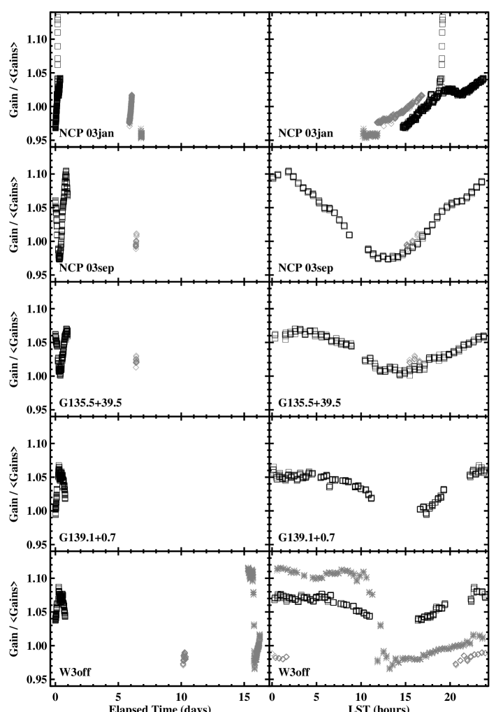
Figure 9: Gains versus time for five data sets. The left-hand column shows elapsed time in days from the first observation for each data set. The right-hand column shows Local Sidereal Time (LST) in hours. Different days have different symbols. The top two rows are the North Celestial Pole (NCP) in 2003 January and 2003 September, respectively. G135.5$+$39.5 was observed in 2003 September and the other two, G139.1$+$0.7 and W3off, were observed in 2003 August.

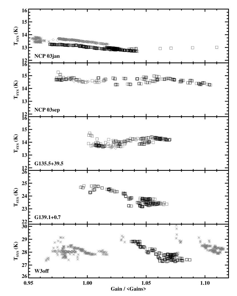
Figure 10: System temperatures versus the normalized gains of Figure 9. Different days have different symbols, the same as in Figure 9.

7.2 The Derived Coefficients and Their Grand Averages

Table 2: Derived Parameters

Source Name	slice angle	$\alpha_{\rm spillover}$	$\alpha_{\rm spot}$	$\alpha_{\rm screen}$	$\alpha_{\rm nearin}$
G139.1$+$0.7	$44.3^{\circ}$	0.089	0.0012	0.0078	0.023
W3off (G133.8$+$0.8)	$49.7^{\circ}$	0.085	0.0007	0.0062	0.021
G135.5$+$39.5	$61.1^{\circ}$	0.092	0.0013	$-$0.0241	0.012
NCP (G122.9$+$27.1)	$46.6^{\circ}$	0.073	$-$0.0008	0.0034	0.012
ADOPTED	$49^{\circ}$	0.087	0.0010	0.0070	0.022

In our least-squares fit for each position, we derive the true profile $T^{*}_{c}$ and a coefficient $\alpha$ for each of the four stray beams. We do this for a set of assumed slice angles, as explained in §6.4. Table 7 presents these fitted coefficients for each of the four positions. We don’t list the formal uncertainties, which are meaninglessly small because even though there is a huge number of independent points in the fit (e.g., for 200 spectra with 400 channels each there are 80000 data) there is a large correlation among spectra taken nearby in time. Rather, the coefficient uncertainties are better estimated from the variation among derived values for the four positions together with consideration of each coefficient’s contribution to each source’s profile. The last line in the table lists our adopted coefficient values.

The largest contaminating beam area is the spillover, whose integrated beam response $\alpha_{spillover}$ is almost $10\%$ of the main beam’s. The screen’s integrated beam response is smaller by a factor of about 12 and the spot’s response is even smaller. The spot and the spillover cover fairly similar regions in realistic situations, so usually the spot’s contribution to the observed 21 cm line profile should be unimportant. This is not necessarily true for the screen, however, because it lies close to the main beam and the 21 cm line intensity here might be much higher than that covered by the spillover—or vice-versa.

In principle, conservation of energy requires that the power removed from the spillover by the screen should appear in the screen component. That is, with a slice angle of $49^{\circ}$, we should have

$$\frac{49}{360}=\frac{\alpha_{\rm screen}}{\alpha_{\rm spillover}+\alpha_{\rm screen}}.$$ (11)

The ratio on the left is 0.14 and that on the right is 0.075, so this relationship is not satisfied at the factor-of-two level. This probably means that we have not properly estimated the properties of the screen component.

7.3 Fit Results for Each Source

Figures 11–14 show the application of the above coefficients for the four sources. In each figure there are 12 panels, each showing averages for $30^{\circ}$-wide bins of parallactic angle PA. The bins have nominal centers at (${\rm PA}=15^{\circ}$, $45^{\circ},...$) running down the page and then to the next column; annotations for each panel provide the actual ranges of PA and LST, together with the number of spectra measured in each bin. Within each panel there are seven line profiles, which include data and residuals (in black) and predicted components (in gray). Some predicted profiles are scaled up in intensity by the factors shown on the left; otherwise they would not be discernible. Within each panel, from top to bottom the profiles are:

1. In black, the observed residual profile $T^{\rm resid}_{c,s}=T^{o}_{c,s}/G^{*}_{s}-T^{*}_{c}$, which is the total predicted contribution of GBT sidelobes. It is obtained by subtracting the derived “true spectrum” from each gain-corrected observed spectrum.

2. In gray, the sum $T^{\rm stray}_{c,s}$ of the four predicted coefficient contributions (“TOT”), which are the next four spectra.

3. In gray, the predicted spillover contribution (“SPIL”).

4. In gray, the predicted spot contribution (“SPOT”).

5. In gray, the predicted Nearin diffraction ring contribution (“NEAR”). This can be negative because we modelled the diffraction ring to have zero net gain; rather, it is a spatial difference.

6. In gray, the predicted screen contribution (“SCRN”).

7. In black, the difference between observed and predicted sidelobe spectra of (1) and (2) above, i.e., $\Delta T_{c,s}=T^{\rm resid}_{c,s}-T^{\rm stray}_{c,s}$. If the predicted spectra are accurate, then this difference is zero.

For the two Galactic plane positions of Figures 11 and 12, the difference $\Delta T_{c,s}$ is quite small. For the high-latitude positions the difference has systematic nonzero features. These amount to perhaps 1/4 of the observed residual profile $T^{\rm resid}_{c,s}$. This reveals inadequacies in our modelling of the sidelobes. Examining these figures shows that the spillover contribution, which covers large velocity ranges and is spectrally smooth, tends to be well-predicted. Most of the residuals cover smaller velocity ranges and have considerable spectral structure.

For example, consider the results for G135.5$+$39.5. The spillover contribution, which comes from large angular distances, covers wide velocity ranges, from $\sim$$-30$ to $\sim$$+10$ km s^-1; in contrast, most of the nonzero $\Delta T_{c,s}$ occurs in a smaller velocity range typically centered on $\sim$$+5$ km s^-1. This narrower range is where the line profile itself is strong. This implies that the inadequacies lie close to the main beam, and in particular imply that the situation is more complicated than the screen and diffraction-ring models we use.

All of this strongly suggests that our predictions from the screen and Nearin components, which lie close to the main beam and occupy small sky areas, are not accurate. Obtaining this near-in beam structure requires very sensitive and high-dynamic range maps of a strong, unresolved source. The Sun is unsuitable because of its large angular diameter. The source Cas A is suitable. However, while obtaining sensitivity requires integration time—which is in principle possible—dealing with the required dynamic range is very difficult. Classically, the dynamic-range problem has been successfully solved only using an interferometric technique (Hartsuijker et al., 1972).

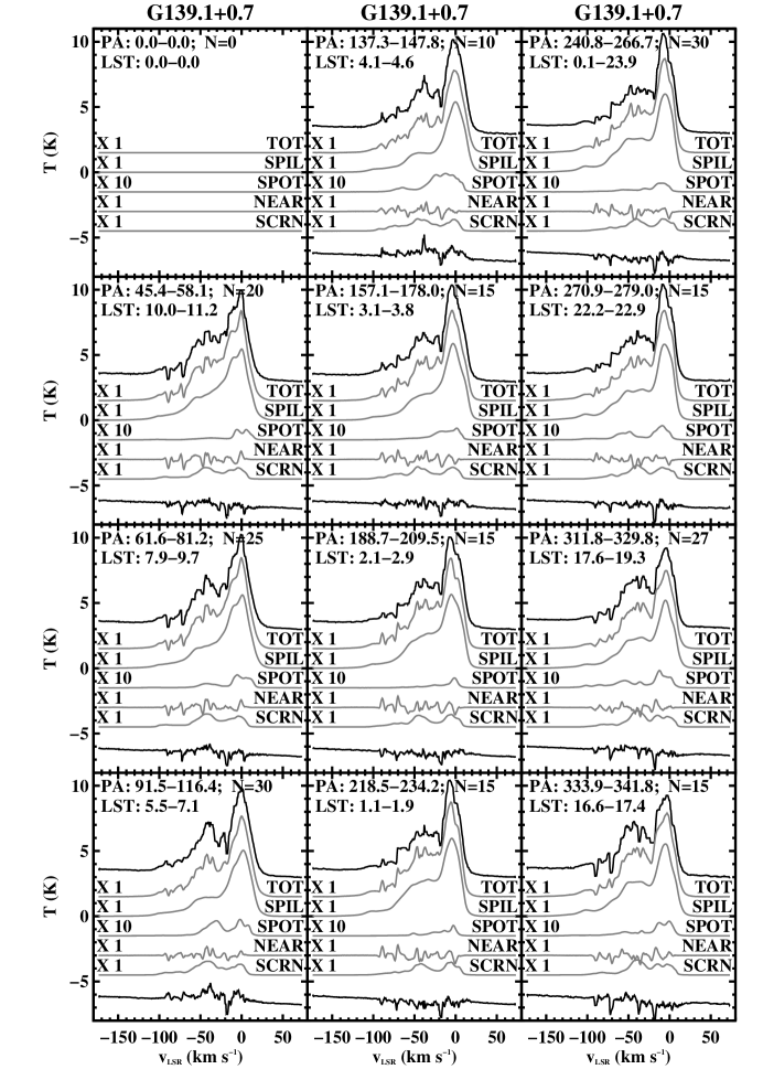
Figure 11: Observed and predicted sidelobe contributions for G139.1$+$0.7. Each panel shows the averages for $30^{\circ}$-wide bins of parallactic angle PA, with successive bins running down the page and then to the next column. The top curve (in black) in each panel is the total observed sidelobe contribution; the next curves, in gray, are the predicted sidelobe contributions; the bottom curve, in black, is the difference between the total observed and predicted contributions. For more details, see text (§7.3).

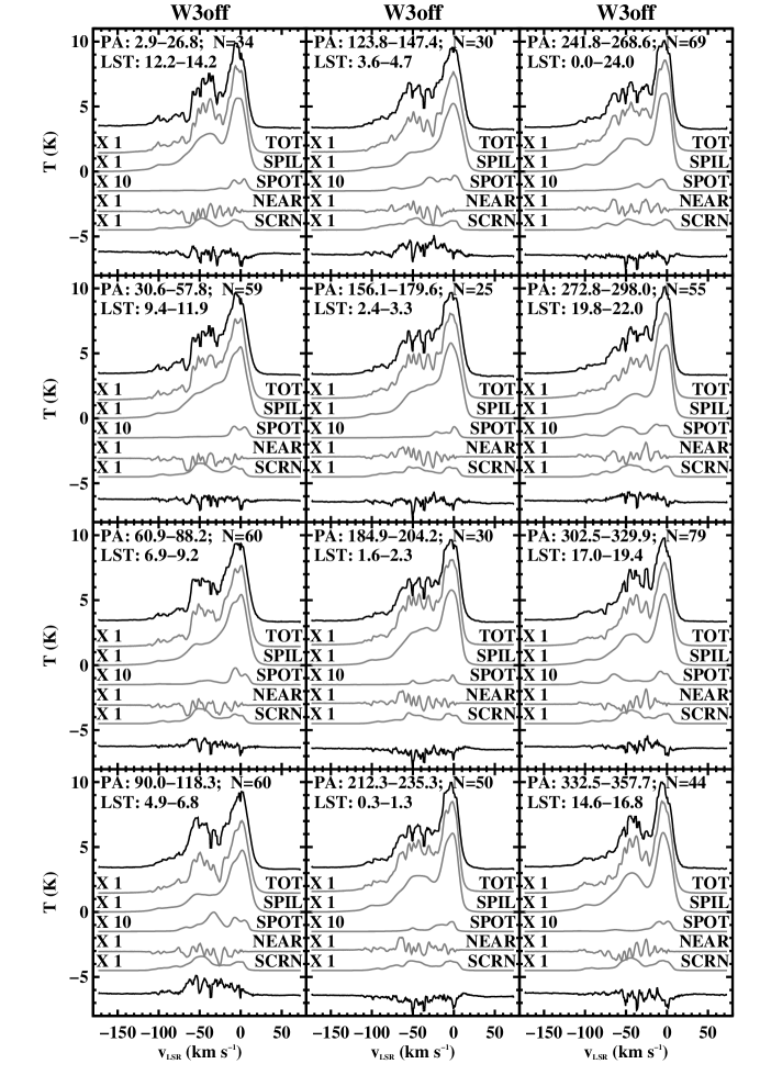
Figure 12: Observed and predicted sidelobe contributions for W3off. Each panel shows the averages for $30^{\circ}$-wide bins of parallactic angle PA, with successive bins running down the page and then to the next column. The top curve (in black) in each panel is the total observed sidelobe contribution; the next curves, in gray, are the predicted sidelobe contributions; the bottom curve, in black, is the difference between the total observed and predicted contributions. For more details, see text (§7.3).

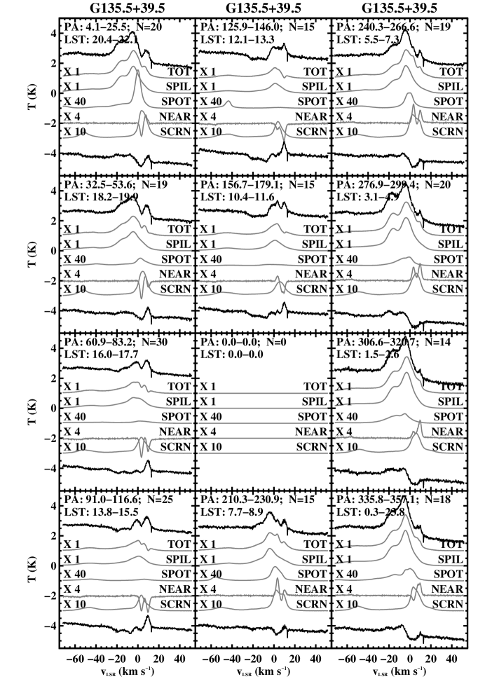
Figure 13: Observed and predicted sidelobe contributions for G135.5$+$39.5. Each panel shows the averages for $30^{\circ}$-wide bins of parallactic angle PA, with successive bins running down the page and then to the next column. The top curve (in black) in each panel is the total observed sidelobe contribution; the next curves, in gray, are the predicted sidelobe contributions; the bottom curve, in black, is the difference between the total observed and predicted contributions. For more details, see text (§7.3).

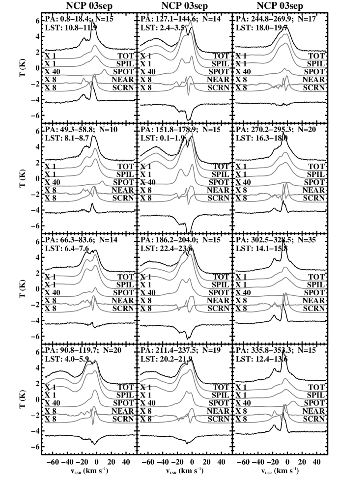
Figure 14: Observed and predicted sidelobe contributions for the NCP data of 2003 September. Each panel shows the averages for $30^{\circ}$-wide bins of parallactic angle PA, with successive bins running down the page and then to the next column. The top curve (in black) in each panel is the total observed sidelobe contribution; the next curves, in gray, are the predicted sidelobe contributions; the bottom curve, in black, is the difference between the total observed and predicted contributions. For more details, see text (§7.3).

8 THE ACCURACY OF STOKES $V$ 21 CM LINE PROFILES

Above, in §3 and Figure 3, we found the measured Stokes $V$ profiles at the NCP to change significantly with time. This shows that the Stokes $I$ sidelobes are partially circularly polarized. Our main interest in using the GBT for 21 cm line work is measuring magnetic fields using Zeeman splitting, which requires measuring Stokes $V$. The 21 cm line velocity changes with position. Angular structure in the Stokes $V$ beam and sidelobes makes the two circular polarizations sample slightly different velocities, and this mimics Zeeman splitting. In this section, we explore the seriousness of this effect for the GBT.

8.1 Stokes $V$ Sidelobes Related to the Secondary Reflector

Figure 15: Stokes $V$ analog for Figure 4. Four Stokes $V$ scans through the Sun in AZ/ZA great-circle offset coordinates. In the left panel we plot the measured antenna temperatures versus the angular offsets from the main beam center. In the right panel, the azimuthal thicknesses of the lines are proportional to the measured temperatures; the dashed circle represents the approximate boundary of the secondary reflector as seen by the feed.. The begin and end points of the legs are labelled on each panel by “,0” and “,1”, respectively.. On the left panel, the arrows lie $5^{\circ}$ outside the dashed circle. On both panels, the spot marks the Arago spot.

Figure 15, left panel, exhibits Stokes $I$ versus AZ/ZA great-circle offset coordinates for the same four scans through the Sun that are shown in Figure 4. These data are for 2003 September 19. The data for 2003 September 7 are similar, but not quite identical; we are unsure whether the differences (which are not very big) are real. Nevertheless, there exists real structure in the Stokes $V$ scans. We mention three notable features:

1. The spillover ring exhibits changes in Stokes $V$ on angular scales ranging downward from about 2 degrees. This structure is readily visible as apparently random wiggles on the left panel of Figure 15, particular for Leg 0.

2. The screen component—i.e., structure within a few degrees of the main beam—exhibits significant, rapidly varying Stokes $V$ structure. Especially prominent are Legs 2 and 0. The Stokes $V$ fractional polarizations are $\sim$25% for the small negative ZA offsets portion of Leg 2 and range from $10\%$ to $20\%$ for the other scans. Near beam center, Leg 0 exhibits a well-defined positive/negative lobe with peaks centered near offsets of a few degrees.

3. The Arago spot, which is centered near $\Delta{\rm ZA}=12^{\circ}$ on Leg 2 (marked with the black spot on Figures 4 and 15), exhibits classical beam squint in Stokes $V$, with the Stokes $V$ intensity crossing zero where Stokes $I$ is maximum. Moreover, the spot’s diffraction rings also exhibit beam squint. The fractional squint peak-to-peak ($I$,$V$) intensities are about $(67,7)$ K and $(10,2.5)$ K for the spot and its first sidelobe, respectively; these correspond to fractional polarizations ($\sim$10%, 25%). The spot’s angular diameter is about 1 degree and the angular distance of the spot’s sidelobe from its peak is about 2 degrees.

8.2 Stokes $V$ Structure of the Primary Beam

Figure 16 is the Stokes $V$ analog of Figure 8. It represents the GBT Stokes $V$ main-beam diffraction rings in two ways, with intensity versus position offset for four observed legs in the left panel and a map in the right. The main beam squint is clear, with the center of the positive lobe centered at about $\phi\approx 205^{\circ}$. The data were taken at ${\rm ZA}\approx 26^{\circ}$; the data of Figure 1 imply $\phi\approx 250^{\circ}$ at ${\rm ZA}\approx 26^{\circ}$. This difference in $\phi$, about $45^{\circ}$, is uncomfortably large and suggests that the squint direction depends on more than just ZA.

The first diffraction ring, which is centered $\sim$$20^{\circ}$ from beam center, exhibits a weak Stokes $V$ signature which is roughly opposite in sign to (and is more complicated than) the main beam’s squint pattern. We don’t show it because the signal/noise is too poor to derive the details.

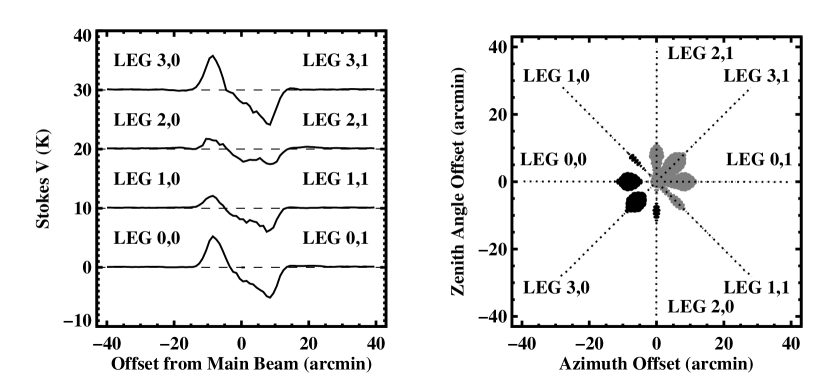
Figure 16: Stokes $V$ analog of Figure 8: Four Stokes $V$ scans (“Legs”) through Cas A in AZ/ZA great-circle offset coordinates, showing the main beam squint. In the left panel we plot the measured antenna temperatures versus the angular offsets from the main beam center. In the right panel, the thicknesses of the lines are proportional to the measured temperatures; black is positive and gray is negative. The begin and end points of the legs are labelled on each panel.

8.3 Stokes $V$ Problems for Each Source

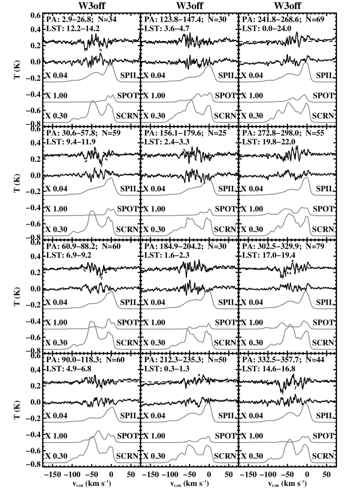
Figure 17: Stokes $V$ (top two profiles) and predicted Stokes $I$ sidelobe contributions for W3off. Each panel shows the averages for $30^{\circ}$-wide bins of parallactic angle PA, with successive bins running down the page and then to the next column. The top curve in each panel is the bin-average Stokes $V$ profile; the next is that profile, corrected for main-beam squint. The next three profiles, in gray, are the predicted Stokes $I$ contributions from spillover (“SPIL”), the Arago spot (“SPOT”), and the screen (“SCRN”), respectively, multiplied by the factors given on the left-hand side for each profiles.

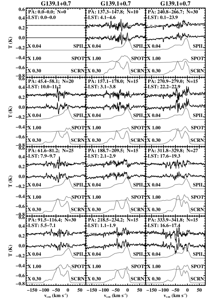
Figure 18: Stokes $V$ (top two profiles) and predicted Stokes $I$ sidelobe contributions for G139.1$+$0.7. Each panel shows the averages for $30^{\circ}$-wide bins of parallactic angle PA, with successive bins running down the page and then to the next column. The top curve in each panel is the bin-average Stokes $V$ profile; the next is that profile, corrected for main-beam squint. The next three profiles, in gray, are the predicted Stokes $I$ contributions from spillover (“SPIL”), the Arago spot (“SPOT”), and the screen (“SCRN”), respectively, multiplied by the factors given on the left-hand side for each profiles.

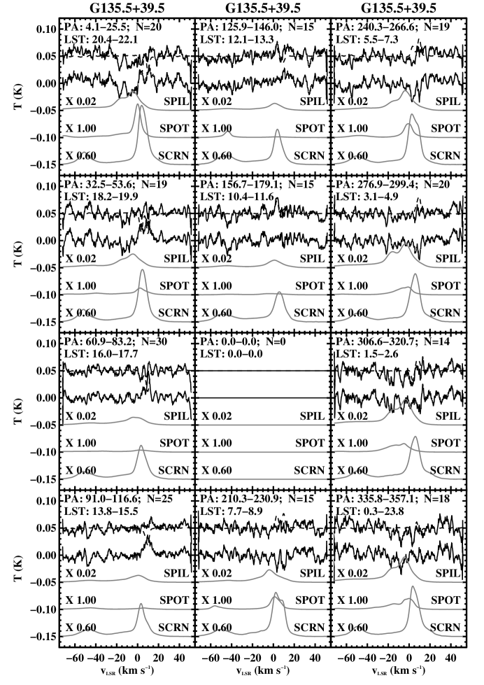
Figure 19: Stokes $V$ (top two profiles) and predicted Stokes $I$ sidelobe contributions for G135.5$+$39.5. Each panel shows the averages for $30^{\circ}$-wide bins of parallactic angle PA, with successive bins running down the page and then to the next column. The top curve in each panel is the bin-average Stokes $V$ profile; the next is that profile, corrected for main-beam squint. The next three profiles, in gray, are the predicted Stokes $I$ contributions from spillover (“SPIL”), the Arago spot (“SPOT”), and the screen (“SCRN”), respectively, multiplied by the factors given on the left-hand side for each profiles.

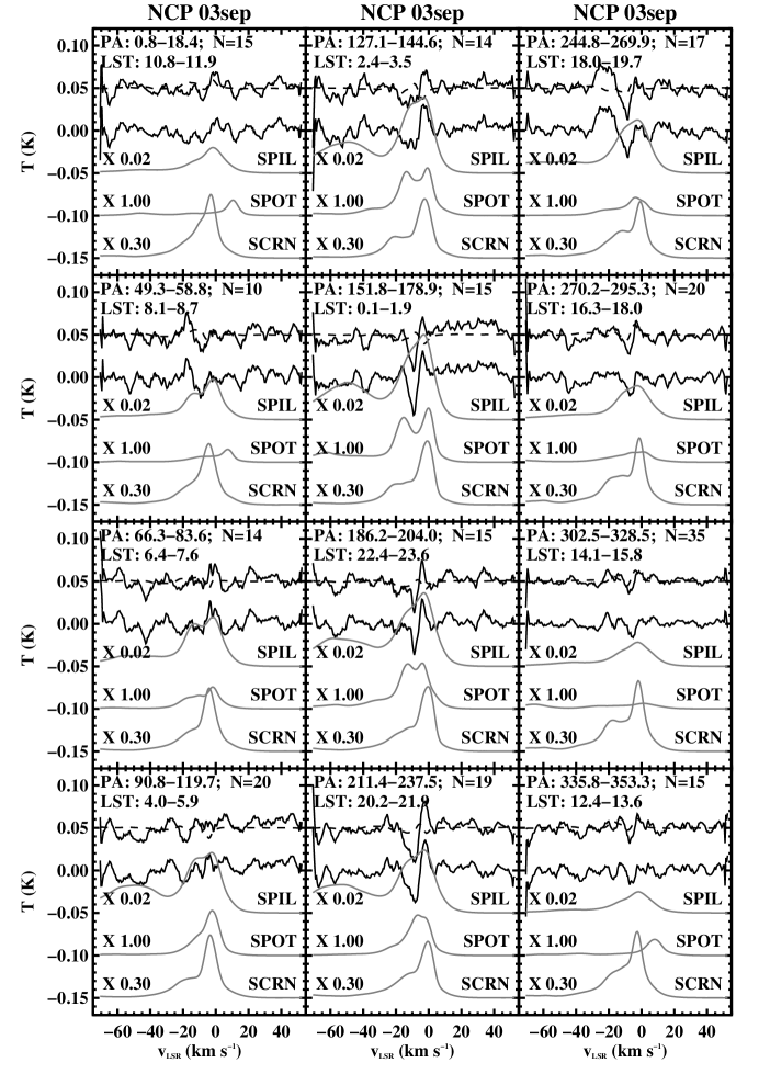
Figure 20: Stokes $V$ (top two profiles) and predicted Stokes $I$ sidelobe contributions for the NCP. Each panel shows the averages for $30^{\circ}$-wide bins of parallactic angle PA, with successive bins running down the page and then to the next column. The top curve in each panel is the bin-average Stokes $V$ profile; the next is that profile, corrected for main-beam squint. The next three profiles, in gray, are the predicted Stokes $I$ contributions from spillover (“SPIL”), the Arago spot (“SPOT”), and the screen (“SCRN”), respectively, multiplied by the factors given on the left-hand side for each profiles.

Figures 17–20 present PA-binned Stokes $V$ profiles together with the predicted Stokes $I$ profiles from the four sidelobe contributions for the four sources. In each figure there are 12 panels, each showing averages for $30^{\circ}$-wide bins of parallactic angle PA. The bins have nominal centers at (${\rm PA}=15^{\circ}$, $45^{\circ},...$) running down the page and then to the next column; annotations for each panel provide the actual ranges of PA and LST, together with the number of spectra measured in each bin.

Within each panel there are five line profiles, which include two Stokes $V$ profiles (in black) and three predicted Stokes $I$ profiles for different sidelobe components (in gray). The predicted profiles are scaled in intensity by the factors shown on the left. The spillover component is generally scaled down by a factor $\sim$20–40 and the screen component by a factor $\sim$2–3; otherwise they would not fit on the panels. Within each panel, from top to bottom the profiles are:

1. In black, the Stokes $V$ profile.

2. In black, the Stokes $V$ profile corrected for main-beam squint.

3. In gray, the predicted Stokes $I$ spillover contribution (“SPIL”), scaled down by a factor $\sim$20–40 as indicated.

4. In gray, the predicted Stokes $I$ spot contribution (“SPOT”).

5. In gray, the predicted Stokes $I$ screen contribution (“SCRN”), scaled down by a factor $\sim$2–3 as indicated.

6. We don’t show the predicted Nearin contribution because it covers roughly the same velocity range as the screen contribution, but has more complicated structure.

First, consider the main-beam squint correction. In some bins it makes a huge improvement. Examples include the ${\rm PA}=272.8^{\circ}{\rm-}298.0^{\circ}$ bin for W3off, the ${\rm PA}=311.8^{\circ}{\rm-}329.8^{\circ}$ bin for G139.1$+$0.7, and the ${\rm PA}=125.9^{\circ}{\rm-}146.0^{\circ}$ bin for G135.5$+$39.5. In most cases, though, its correction represents only a small portion of the time-variable systematic errors in the Stokes $V$ profiles.

We conclude that the circularly-polarized portions of the four spillover contributions are responsible for most of the Stokes $V$ inaccuracies. Figures 17–20 provide some clues about which components are serious contributors to these errors. We consider, first, the Spillover and Spot contributions.

1. The Spillover component. Generally, the Stokes $I$ Spillover profile covers a large velocity range. By inspection, this allows us to see that the Stokes $V$ problems do not scale very well with the Stokes $I$ spillover intensity. For example, the ${\rm PA}=123.8^{\circ}{\rm-}147.4^{\circ}$ bin for W3off has severe Stokes $V$ wiggles for $v_{\rm\scriptstyle LSR}\lesssim-25$ km s^-1, where the Stokes $I$ Spillover profile is weak; more generally for this source, the Stokes $I$ Spillover profile changes quite a bit in intensity for $v_{\rm\scriptstyle LSR}\lesssim-25$ km s^-1, but the wiggle amplitudes in the Stokes $V$ spectra don’t track these changes. The same general statement applies to G139.1$+$0.7. Similarly, for the two high-latitude sources the Stokes $I$ spillover amplitude varies considerably with PA, but the Stokes $V$ wiggles don’t track these variations.

2. The Spot component. Generally, the Stokes $I$ Spot profile covers a smaller velocity range than the Spillover profile and is less spectrally smooth. This makes it easier to see that the Stokes $V$ problems are not well-correlated with the Stokes $I$ spot profile intensity. Clear examples include the ${\rm PA}=156.1^{\circ}{\rm-}179.6^{\circ}$ bin for W3off, the ${\rm PA}=157.1^{\circ}{\rm-}178.0^{\circ}$ bin for G139.1$+$0.7, and many of the bins for the two high-latitude sources.

3. We conclude that most of the Stokes $V$ wiggles do not come from the either the Spillover or the Spot lobe.

By the process of elimination, this leaves the Screen and Nearin components. Consider, first, the possible contribution to Stokes $V$ from the Nearin component, i.e., the diffraction rings. We concluded above in §5 that the integrated response of the diffraction rings is $\lesssim 1\%$ that of the main beam. In §8.2 we found that the diffraction rings are almost unmeasurable in Stokes $V$ and are $\lesssim 20$ times weaker than the main-beam squint. We have seen that the main-beam squint accounts for only a fraction of the observed Stokes $V$ wiggles. The contribution from the diffraction rings should be smaller. We conclude that the diffraction rings contribute insignificantly to the Stokes $V$ wiggles.

8.4 The Culprit Is the Screen Component

Again by process of elimination, we are left with the Screen component as the culprit that produces the extraneous Stokes $V$ wiggles. This conclusion makes quantitative sense. First, the integrated beam response of the Screen component is roughly $1\%$ the main beam’s (§6.2; Table 2). This seems small, but the Stokes $V$ wiggles are of order $10^{-4}$ the Stokes $I$ amplitude, and the Screen component is much more highly polarized than the main beam. Above, in §8.1, we concluded its Stokes $V$ fractional polarization reaches $\sim$25%. Moreover, this polarization changes over the size of the Screen component, which is a ring of radius $\sim$$2.8^{\circ}$ (eq. [4]). Thus, it samples changes in the 21 cm profiles over much larger angles than the main beam does.

Unfortunately, our estimate of the screen beam is very rough. It is very difficult to accurately measure the screen component—not only in Stokes $I$, as we remarked above in §7.3, but even more so in Stokes $V$. This means that we cannot present any hard and fast rule about its effect. We can only offer a rule of thumb, which we base on comparing the Stokes $V$ wiggle amplitude with the predicted Stokes $I$ screen profile of Figures 17–20. In these figures, the Stokes $V$ wiggle is of order 0.2 times the predicted screen Stokes $I$ profile. So we can offer the following:

1. For Stokes $V$ measurements in narrow ranges of parallactic angle PA, results can be trusted if they are stronger than $\sim$0.2 the predicted Stokes $I$ screen component.

2. Averaging over larger ranges of parallactic angle PA helps greatly. If one has sampling of the full range of PA, then the Stokes $V$ results are much more reliable.

9 SUMMARY AND PERSPECTIVE

9.1 Summary

We sampled the GBT sidelobes and used structural and physical considerations to define four sidelobe components. Three of these are related to the feed’s illumination of the secondary reflector: the spillover, the spot, and the screen components (§4). A fourth component, which we call the nearin component, is related to the diffraction rings (§5). We applied a least-squares procedure (§6, §7) to full hour-angle coverage of 21 cm line data for four positions to obtain the amplitude of these components, and also to obtain the errors in calibrated gains for each spectrum and the true profile for each position.

We find the following items of importance for accurate 21 cm line profiles measured by the GBT:

1. We find intrinsic differences between calibrated intensity for GBT versus LAB profiles at the $\sim$60% level (Table 1), which we attribute to the higher main-beam efficiency of the GBT; this, in turn, is a direct result of its clear, unblocked aperture.

2. We find systematic time variations i n the calibrated gain (Figure 9), which means that GBT 21 cm line profile intensities cannot be relied on at the $10\%$ level.

3. The combination of the spillover, spot, and screen sidelobes has an area-integrated beam response which is almost $10\%$ that of the main beam (Table 2). These can produce significant inaccuracy in observed Stokes $I$ 21 cm line profiles (stray radiation).

4. We use the solutions for the sidelobe beam responses, together with the LAB survey, to predict and remove the 21 cm line contaminants with fair accuracy (§7.3).

5. The distant sidelobes also contribute to Stokes $V$ 21 cm line profiles (§8). In particular, the screen component contributes a currently uncorrectable contaminant to the Stokes $V$ profiles. This has amplitude $\sim$20% of its Stokes $I$ counterpart, so GBT Stokes $V$ 21 cm line profiles cannot be trusted at this level unless they are averaged over significant ranges of parallactic angle.

In summary, 21 cm line profiles in both Stokes $I$ and Stokes $V$ contain significant contaminants. For Stokes $I$, these can be removed with some success with the procedure presented in this paper. Uncertainties in the predicted contaminants are dominated by our inaccurate knowledge of the screen component. This can, in principle, be measured more accurately, but doing so requires high dynamic range measurements of an unresolved source; these are probably feasible only using the interferometric technique of Hartsuijker et al. (1972).

9.2 Perspective

We find it ironic that, historically, one of the arguments for the clear-aperture design of the GBT was the enhanced accuracy of 21 cm line profiles. The purity of its clear-aperture design is spoiled by the use of a Cassegrain system, with its secondary reflector. Upon reflection, we see that using the GBT in a prime-focus mode would retrieve most, perhaps all, of this purity. One would pay for this with a large beam squint in Stokes $V$—but this would be a predictably reliable and straightforward correction. It seems to us that using the GBT in prime-focus mode would provide more accurate 21 cm line profiles in both Stokes $I$ and $V$ than performing a series of uncertain and perhaps time-variable corrections to profiles measured with the Cassegrain system.

References

- Fisher (1991) Fisher, R. 1991, Spectral Processor Manual (Green Bank, WV: NRAO)
- Hartmann (1994) Hartmann, D. 1994, Ph.D. thesis, Leiden Univ.
- Hartmann et al. (1996) Hartmann, D., Kalberla, P. M. W., Burton, W. B., & Mebold, U. 1996, A&AS, 119, 115
- Hartsuijker et al. (1972) Hartsuijker, A. P., Baars, J. W. M., Drenth, S., & Gelato-Volders, L. 1972, IEEE Trans. Antenn. Prop., 20, 166
- Heiles et al. (2003) Heiles, C., Robishaw, T., Troland, T., & Roshi, D. A. 2003, GBT Commissioning Memos, Memo 23
- Heiles & Troland (2003) Heiles, C., & Troland, T. H. 2003, ApJS, 145, 329
- Heiles et al. (2001) Heiles, C., et al. 2001, PASP, 113, 1247
- Jackson et al. (2003) Jackson, T., Werner, M., & Gautier, T. N., III 2003, ApJS, 149, 365
- Kalberla et al. (2005) Kalberla, P. M. W., Burton, W. B., Hartmann, D., Arnal, E. M., Bajaja, E., Morras, R., & Pöppel, W. G. L. 2005, A&A, 440, 775
- Kraus (1988) Kraus, J. D. 1988, Antennas (2nd ed.; New York: McGraw-Hill)
- Lockman & Condon (2005) Lockman, F. J., & Condon, J. J. 2005, AJ, 129, 1968
- Norrod (1990) Norrod, R. D. 1990, GBT Memo 41
- Norrod & Srikanth (1996) Norrod, R. D., & Srikanth, S. 1996, GBT Memo 155
- Press et al. (1992) Press, W. H., Teukolsky, S. A., Vetterling, W. T., & Flannery, B. P. 1992, Numerical Recipes in FORTRAN: The Art of Scientific Computing (2nd ed.; Cambridge: Cambridge Univ. Press)
- Sommerfeld (1954) Sommerfeld, A. 1954, Optics: Lectures on Theortical Physics, Vol. IV (New York: Academic Press)