The Double Life of Thermal QCD

Abstract

We study the gravity dual of a thermal gauge theory whose behavior parallels that of thermal QCD in the far IR. The UV of our theory has infinite degrees of freedom. We holographically renormalize the supergravity action to compute the stress tensor of the dual gauge theory with fundamental flavors incorporating the logarithmic running of the gauge coupling. From the stress tensor we obtain the shear viscosity and the entropy of the medium at a temperature T, and investigate the violation of the bound for the viscosity to the entropy ratio. This is a shortened and simplified companion paper to hep-th/0902.1540, and is based on the talks given by M. Mia at the “Strong and Electroweak Matter 2008” workshop and the McGill workshop on “AdS/CFT, Condensed Matter and QCD” in the fall of 2008.

1 Introduction

Strongly coupled Quark Gluon Plasma (QGP) poses theoretically challenging yet experimentally accessible questions. The formation of QGP at RHIC is an example where theoretical descriptions are completely lacking at low energies because our perturbative techniques fail at strong couplings. However probing the nonperturbative regime of large $N$ gauge theory through a gravity dual has led to some interesting results for the physics of the quark gluon plasma. A popular approach so far has been the AdS/CFT correspondence [1], even though QCD is not a conformal field theory at UV. However, for certain gauge theories with running couplings, there exist gravity duals. At zero temperatures these gravity duals are studied with [2] and without [3, 4] fundamental flavors. On the other hand, at high temperatures, there are examples of gravity duals without fundamental flavors in the literature [7]. In this paper we give an example of a gravity dual for a specific thermal gauge theory with fundamental flavors and logarithmically running coupling constants (see also [8]). Our aim here is to study quantities such as shear viscosity, entropy and the viscosity to entropy ratio with our gravity dual.

2 The Duality

The gauge theory that we consider arises from stacking $N$ D3 branes at the tip of a six dimensional conifold with base $T^{1,1}=S^{2}\times S^{3}$, then placing $M$ D5 branes in such a way that it wraps the two cycle $S^{2}$ on the base of the conifold alongwith $N_{f}$ $D7$ branes embedded via so-called Ouyang embedding [2] to introduce fundamental matter [5]. Finally by euclideanising and periodically identifying the time coordinate we can introduce temperature in the gauge theory. However the high temperature, i.e temperature above the deconfinement temperature that we would be interested in, will be generated by inserting a black hole in the dual gravitational backgound [5]. The D3 brane world volume and the unwrapped directions of D5 and D7 branes extends in the four Minkowski directions. Strings can end on any of these branes and the excitation of the strings are described by an $SU(N+M)\times SU(N)$ gauge group with $N_{f}$ flavors. If $g_{1},g_{2}$ denote the gauge couplings of $SU(N+M)$ and $SU(N)$, then they have nontrivial beta functions (at zero temperature) $\frac{\partial}{\partial{\rm log}~{}\Lambda}\left[\frac{4\pi^{2}}{g_{1}^{2}}+\frac{4\pi^{2}}{g_{2}^{2}}\right]=-\frac{3N_{f}}{4}$ and $\frac{\partial}{\partial{\rm log}~{}\Lambda}\left[\frac{4\pi^{2}}{g_{1}^{2}}-\frac{4\pi^{2}}{g_{2}^{2}}\right]=3M\left(1+\frac{3g_{s}N_{f}}{2\pi}~{}{\rm log}\Lambda\right)$. We see that the two gauge couplings run in opposite directions and in the IR $SU(N+M)$ flows to strong coupling. Performing a Seiberg duality transformation, we identify the strongly coupled $SU(N+M)$ with a weakly coupled $SU(N-(M-N_{f}))$ at the IR. We see that not only the number of colors are reduced, but the difference of the size of the gauge group now decreases from $M$ in [3] to $M-N_{f}$. This difference will decrease by the increments of $N_{f}$ until it is smaller than or equal to $N_{f}$. Then there are two possible end points: (a) if $N$ is still greater than zero then we will have an approximately conformal theory, or (b) if $N$ decreases to zero but with finite $M$ left over then we will have a $SU(M)$ theory with $N_{f}$ flavors that confines in the far IR (see [2] for more details). The latter theory, or more particularly the high temperature limit of the latter theory, is what we are interested in and henceforth we will only consider that.

At zero temperature the dual description (assuming of course that in this limit the gauge theory decouples from gravity) involves D7 branes, deformed conifold and fluxes [2]. Due to the underlying RG flows the supergravity description does not capture the choppy cascading nature of the gauge theories! Rather the supergravity description only captures the smooth RG flows in the theory. This would also mean that the actual number of colors in the theory is rather subtle to define. These details are explored in [4, 5].

Once we switch on a temperature in the gauge theory, the dual gravity description loses its simplicity. We can no longer claim that the fluxes, warp factor etc would remain unchanged. Even the internal manifold cannot remain a simple warped deformed conifold any more. All the internal spheres would get squashed, and at $r=0$ there could be both resolution as well as deformation of the two and three cycles respectively. Due to this complicated nature of our background our entire analysis in [5] is based on the following limit:

$$\left(g_{s},~{}g_{s}N_{f},~{}g^{2}_{s}MN_{f},~{}{g_{s}M^{2}\over N}\right)~{}\to~{}0,~{}~{}~{}~{}~{}(g_{s}N,~{}g_{s}M)~{}\to~{}\infty$$ (1)

In [5] we presented our results to ${\cal O}(g_{s}N_{f},g_{s}M^{2}/N)$, and discuss how to extend this to higher orders in $g_{s}N_{f}$ and $g_{s}M^{2}/N$. In the limit where the deformation parameter is small, we show that to ${\cal O}(g_{s}N_{f},g_{s}M^{2}/N)$ we can analytically derive the background taking a resolved conifold geometry. The resolution parameter $a$ depends on $g_{s}N_{f},g_{s}M^{2}/N$ as well as on the horizon radius $r_{h}$ i.e $a=a_{0}+{\cal O}(g_{s}N_{f},g_{s}M^{2}/N,r_{h})$ with $a_{0}$ constant. Our background then has the following form:

$$ds^{2} = {1\over\sqrt{h}}\Big{[}-g_{1}(r)dt^{2}+dx^{2}+dy^{2}+dz^{2}\Big{]}+\sqrt{h}\Big{[}g_{2}(r)^{-1}dr^{2}+d{\cal M}_{5}^{2}\Big{]}$$

$${\widetilde{F}}_{3} = 2M{\bf A_{1}}\left(1+{3g_{s}N_{f}\over 2\pi}~{}{\rm log}~{}r\right)~{}e_{\psi}\wedge\frac{1}{2}\left({\rm sin}~{}\theta_{1}~{}d\theta_{1}\wedge d\phi_{1}-{\bf B_{1}}~{}{\rm sin}~{}\theta_{2}~{}d\theta_{2}\wedge d\phi_{2}\right)$$

$$-{3g_{s}MN_{f}\over 4\pi}{\bf A_{2}}~{}{dr\over r}\wedge e_{\psi}\wedge\left({\rm cot}~{}{\theta_{2}\over 2}~{}{\rm sin}~{}\theta_{2}~{}d\phi_{2}-{\bf B_{2}}~{}{\rm cot}~{}{\theta_{1}\over 2}~{}{\rm sin}~{}\theta_{1}~{}d\phi_{1}\right)$$

$$-{3g_{s}MN_{f}\over 8\pi}{\bf A_{3}}~{}{\rm sin}~{}\theta_{1}~{}{\rm sin}~{}\theta_{2}\left({\rm cot}~{}{\theta_{2}\over 2}~{}d\theta_{1}+{\bf B_{3}}~{}{\rm cot}~{}{\theta_{1}\over 2}~{}d\theta_{2}\right)\wedge d\phi_{1}\wedge d\phi_{2}$$

$$H_{3} = {6g_{s}{\bf A_{4}}M}\Bigg{(}1+\frac{9g_{s}N_{f}}{4\pi}~{}{\rm log}~{}r+\frac{g_{s}N_{f}}{2\pi}~{}{\rm log}~{}{\rm sin}\frac{\theta_{1}}{2}~{}{\rm sin}\frac{\theta_{2}}{2}\Bigg{)}\frac{dr}{r}\wedge\frac{1}{2}\Big{(}{\rm sin}~{}\theta_{1}~{}d\theta_{1}\wedge d\phi_{1}$$

$$-{\bf B_{4}}~{}{\rm sin}~{}\theta_{2}~{}d\theta_{2}\wedge d\phi_{2}\Big{)}+\frac{3g^{2}_{s}MN_{f}}{8\pi}{\bf A_{5}}{\cal D}(r,\psi)\wedge\Bigg{(}{\rm cot}~{}\frac{\theta_{2}}{2}~{}d\theta_{2}-{\bf B_{5}}~{}{\rm cot}~{}\frac{\theta_{1}}{2}~{}d\theta_{1}\Bigg{)}$$

$$C_{0} = {N_{f}\over 4\pi}(\psi-\phi_{1}-\phi_{2}),~{}~{}~{}~{}~{}~{}F_{5}~{}=~{}{1\over g_{s}}\left[d^{4}x\wedge dh^{-1}+\ast(d^{4}x\wedge dh^{-1})\right]$$

$$e^{-\Phi} = {1\over 2g_{s}}\left[{1\over r^{\epsilon_{a}}}-{3\epsilon_{a}a^{2}\over 2r^{2}}-\frac{g_{s}N_{f}}{2\pi}{\rm log}\left({\rm sin}~{}{\theta_{1}\over 2}~{}{\rm sin}~{}{\theta_{2}\over 2}\right)+{\rm constant}\right]$$ (2)

where ${\cal D}(r,\psi)\equiv\frac{dr}{r}\wedge e_{\psi}-\frac{1}{2}de_{\psi}$; $g_{i}$ are the black hole factors; $\epsilon_{a}={3g_{s}N_{f}\over 4\pi}$; ${\bf A}_{i},{\bf B}_{i}$ are ${\cal O}(a^{2},g_{s}N_{f})$ corrections that take us away from the zero temperature Ouyang background [2], and are worked out in details in [5]; and ${\cal M}_{5}$ is a warped resolved conifold with the warp factor:

$$h~{}=~{}{L^{4}\over r^{4-\epsilon_{1}}}~{}+~{}{L^{4}\over r^{4-2\epsilon_{2}}}~{}-~{}{2L^{4}\over r^{4-\epsilon_{2}}}~{}+~{}{L^{4}\over r^{4-r^{\epsilon^{2}_{2}/2}}}~{}\equiv~{}\sum_{\alpha=1}^{4}{L^{4}_{(\alpha)}\over r^{4}_{(\alpha)}}$$ (3)

where $\epsilon_{i},r_{(\alpha)}$ etc are defined as:

$$\epsilon_{1}~{}=~{}{3g_{s}M^{2}\over 2\pi N}+{g_{s}^{2}M^{2}N_{f}\over 8\pi^{2}N}+{3g_{s}^{2}M^{2}N_{f}\over 8\pi N}~{}{\rm log}\left({\rm sin}~{}{\theta_{1}\over 2}{\rm sin}~{}{\theta_{2}\over 2}\right),~{}~{}\epsilon_{2}~{}=~{}{g_{s}M\over\pi}\sqrt{2N_{f}\over N}$$

$$~{}~{}~{}~{}~{}~{}~{}~{}~{}~{}~{}r_{(\alpha)}=r^{1-\epsilon_{(\alpha)}},~{}~{}\epsilon_{(1)}={\epsilon_{1}\over 4},~{}~{}\epsilon_{(2)}={\epsilon_{2}\over 2},~{}~{}\epsilon_{(3)}={\epsilon_{2}\over 4},~{}~{}\epsilon_{(4)}={\epsilon^{2}_{2}\over 8}$$

$$~{}~{}~{}~{}~{}~{}~{}~{}~{}~{}~{}r_{(\pm\alpha)}=r^{1\mp\epsilon_{(\alpha)}},~{}~{}~{}L_{(1)}=L_{(2)}=L_{(4)}=L^{4},~{}~{}~{}L_{(3)}=-2L^{4}$$ (4)

and $L^{4}$ is defined in the same way as in the AdS/CFT correspondence. The D7 branes are embedded via Ouyang embedding in this background. Note that our analysis to this order is analytic, but beyond this order we loose all analytic control and we can only find the background numerically (see also [7] for the background without flavor D7 branes and [9] for the background with flavor branes). Furthermore the ${\rm log}~{}r$ dependences of all the fluxes, warp factor and dilaton is only for regions close to the D7 brane. To get a good behavior at far infinity we need to embed the whole system in F-theory [10]. That would mean inserting extra $24-N_{f}$ seven branes at infinity; and then all the fluxes would go as inverse powers of $r$ at large $r$. In fact in [5] we made a concrete prediction for the large $r$ warp factor: it is given by (3) except that the sum over $\alpha$ now ranges from $-\infty$ to $+\infty$. This way we can get rid of possible Landau poles (or naked singularities) in the background (see also [11]). On the other hand for finite $g_{s}N_{f},g_{s}M^{2}/N$ the small $r$ behavior is almost identical to (3). However we couldn’t derive the precise form for the large $r$ behavior of the warp factor. Therefore in [5] we only speculated a possible inverse $r$ behavior for the warp factor.

Once we know the dual background we can say that the Hilbert space of the gauge theory can be obtained from the Hilbert space of the string theory on this geometry. In fact the dual supergravity background captures the strongly coupled gauge theory where we expect the RG flow to be smooth without any choppy Seiberg dualities, although we might be able to interpret the strongly coupled gauge theory also as some kind of approximate cascading theory.

As we now know very well, the UV completion of cascading type theories require infinite degrees of freedom. Once we have infinite degrees of freedom at the UV, we no longer expect a finite boundary action from supergravity analysis! What we need is to regularise and renormalise the supergravity boundary action so that finite correlation functions could be extracted. This would also mean that the usual Witten type proposal [12] for the AdS/CFT correspondence can be re-expressed in terms of the boundary variables to give us the complete picture. Therefore we can rewrite the ansatze proposed by Witten et al [12] for our background geometry to take the following Wilsonian form:

$${\cal Z}_{\rm QCD}[\phi_{0}] ~{}\equiv ~{}\langle{\rm exp}\int_{M^{4}}\phi_{0}{\cal O}\rangle~{}=~{}{\cal Z}_{\rm total}[\phi_{0}]$$ (5)

$$~{}\equiv ~{}{\rm exp}(S_{\rm total}[\phi_{0}]+S_{\rm GH}+S_{\rm counterterm})~{}\equiv~{}{\rm exp}~{}S_{\rm ren}[\phi_{0}]$$

where $M^{4}$ is Minkowski manifold, $S_{\rm total}$ is the low energy type IIB action defined in the string frame, $\phi_{0}$ is the fluctuation over a given background, $S_{\rm GH}$ is the Gibbons-Hawking boundary term [14] and $S_{\rm counterterm}$ is the counter-term action added to renormalise the action.

The interesting part now is that we can define two classes of theories in this kind of backgrounds by introducing a cut-off at $r=r_{c}$:

$\bullet$ The first class is to analyse the theory right at the usual boundary where $r_{c}\to\infty$. This is the standard picture where there are infinite degrees of freedom at the boundary, and the theory has a smooth RG flow from UV to IR till it confines (at least from the weakly coupled gravity dual).

$\bullet$ The second class is to analyse theories by specifying the degrees of freedom at generic $r_{c}$ and then defining the theories at the boundary. All these theories would meet the cascading theory at certain scales under RG flows. The gravity duals of these theories are the usual resolved-deformed conifold geometries cut-off at various $r_{c}$ with appropriate UV caps added (or, alternatively, degrees of freedom specified). These UV caps are non-trivial geometries added to the resolved-deformed conifold geometry from $r=r_{c}$ to $r=\infty$. In addition to that, both these classes of theories ought to have appropriate number of seven branes so that all the Landau poles could be removed.

We can also say that the boundary degrees of freedom are now given by ${\cal N}_{\rm uv}$ where ${\cal N}_{\rm uv}=\epsilon^{-n},\epsilon\to 0$ and $n>>1$ specifies the parent cascading theory. For all other theories that we define at the boundary $r=\infty$, by cutting off the geometry at $r=r_{c}$, will have ${\cal N}_{\rm uv}$ going as ${\cal N}_{\rm uv}=\epsilon^{-n}$ but now $n\geq 1$. Yet another interesting thing about all these theories is that any thermodynamical quantitities defined in these theories will be completely independent of the cut-off $r_{c}$ and only depend on the temperature $T$ (with an exponentially small dependences on the boundary degrees of freedom)! This will be briefly demonstrated in the next section (see [5] for the full exposition).

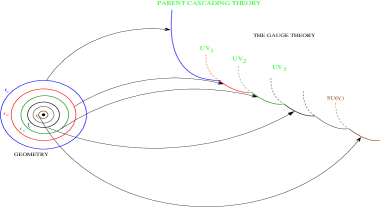
Figure 1: A very approximate way to denote all the UV completed theories that we could study in our framework by cutting off the geometry at various $r=r_{c}$. For a more correct illustration of the situation see [5]. The outermost blue curves on both sides denote the parent cascading theory.

3 The Stress Tensor

One of the important thermodynamical quantity to extract from our background would be the stress tensor. As the stress tensor couples to the metric, it’s expectation value is obtained from the renormalised action $S_{\rm ren}$ via $\langle T^{ij}(\Lambda_{c})\rangle=\frac{\delta S_{\rm ren}[l_{ij}]}{\delta l_{ij}}\Big{|}_{l_{ij}=0}$ where $l_{ij}$ is the four dimensional effective metric induced by the ten dimensional metric of the form (2) by approximating the metric first by a five dimensional slice and then taking the required pull-back (see [5] for details on the procedure). At every fixed $r$ the five dimensional metric induces a four dimensional metric and with appropriate rescaling of the time coordinate, we can view this effective four dimensional metric as a flat Minkowski metric (with possible perturbations). If $O_{ij}$ denote the perturbations on the background by quark strings that stretch from the D7 branes to the horizon of the black hole, then writing the supergravity action up to quadratic order in $O_{ij}$; using integration by parts together with appropriate Gibbons-Hawking terms; and holographically renormalising the subsequent action, we obtain:

$$T^{mm}_{{\rm medium}+{\rm quark}}=\int\frac{d^{4}q}{(2\pi)^{4}}\sum_{\alpha,\beta}\Bigg{\{}({H}_{|\alpha|}^{mn}+{H}_{|\alpha|}^{nm})s_{nn}^{(4)[\beta]}-4({K}_{|\alpha|}^{mn}+{K}_{|\alpha|}^{nm})s_{nn}^{(4)[\beta]}$$

$$~{}~{}~{}~{}~{}~{}~{}~{}~{}~{}~{}+({K}_{|\alpha|}^{mn}+{K}_{|\alpha|}^{nm})s_{nn}^{(5)[\beta]}+\sum_{j=0}^{\infty}~{}\hat{b}^{(\alpha)}_{n(j)}\widetilde{J}^{n}\delta_{nm}e^{-j{\cal N}_{\rm uv}}+{\cal O}({\cal T}e^{-{\cal N}_{uv}})\Bigg{\}}$$ (6)

where ($\hat{b}^{(\alpha)}_{n(j)},{\cal N}_{\rm uv}$) together will specify the full boundary theory for a specific UV complete theory. The quantities $H^{mn},\widetilde{J}^{m},K^{mn}$ etc. with $m,n=0,..,3$ are completely independent of the radial coordinate $r$ and depend on the 3+1 dimensional spacetime coordinates. Note also that the stress tensor depends only on the temperature $T$ and is independent of any cut-offs. The dependence on the UV degrees of freedom is exponentially suppressed, and in the limit ${\cal N}_{\rm uv}=\epsilon^{-n},n>>1$ we reproduce the result for the parent cascading theory.

4 Results and Discussion

With the general formulation of stress tensor (3), which is similar to the AdS/CFT results [16] in the limiting case $M=N_{f}=0$, we can compute the wake a moving quark creates in a plasma with $O_{ij}$ being the metric perturbation due to string (see [17] for an equivalent AdS calculation). Furthermore we can compute the shear viscosity $\eta$ from the Kubo formula with the propagator obtained from the dual partition function (5) and the entropy density $s$ using Wald’s formula. The result for the ratio $\eta/s$ is given by:

$$\frac{\eta}{s} = ~{}{1+\sum_{k=1}^{\infty}\alpha_{k}e^{-4k{\cal N}_{\rm uv}}\over 4\pi+{1\over\pi}~{}{\rm log}^{2}\left(1-{T}^{4}e^{-4{\cal N}_{uv}}\right)}$$ (7)

$$- \frac{c_{3}\kappa}{3L^{2}\left(1-{T}^{4}e^{-4{\cal N}_{uv}}\right)^{3/2}}\left[\frac{{B_{o}}(4\pi^{2}-{\rm log}^{2}~{}C_{o})+4\pi{A_{o}}~{}{\rm log}~{}C_{o}}{\Big{(}4\pi^{2}-{\rm log}^{2}~{}C_{o}\Big{)}^{2}+16\pi^{2}~{}{\rm log}^{2}~{}C_{o}}\right]$$

where ($A_{o},B_{o},C_{o},\alpha_{k}$) are constants that depend on the temperature $T$ and $e^{-{\cal N}_{\rm uv}}$; and $c_{3}$ is the coefficient of the Riemann square term coming from the backreactions of the D7 branes in the background. These have been explicitly worked out in [5]. The $c_{3}$ dependence of the $\eta/s$ ratio first appeared in [18].

With certain choices of parameters ($g_{s}=0.01,N=1000,M=100,N_{f}=3,c_{3}=0.001$) and ignoring ${\cal O}(g_{s}N_{f},g_{s}M^{2}/N)$ corrections to the black hole parameters $g_{i}(r)$ the result for $\eta/s$ is shown in figure 2. It is easy to see that we are violating the celebrated KSS bound [19].

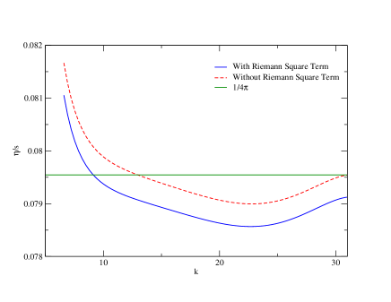
Figure 2: Plot of $\eta/s$ versus the UV degrees of freedom.

The plot in figure 2 is shown for $\eta/s$ with and without Riemann Square term. The x-axis is defined as $k={e^{{\cal N}_{\rm uv}}\over{T}}$ where ${\cal N}_{\rm uv}$ is the UV degrees of freedom and ${T}$ is the temperature of the cascading theories. For the parent cascading theory, and their corresponding family of theories, $k\to\infty$ and we see a violation of the bound (the solid blue line). As $k$ decreases (assuming this is possible!) the red dashed line dips slightly below the $1/4\pi$ axis, but the solid blue line remains considerably below the $1/4\pi$ axis. For $k$ sufficiently small the bound is not violated. However all the models that we studied here and in [5] can only realise the infinite $k$ limit, so that the small $k$ limit depicted in Fig. 2 above is just an extrapolation of (7).

5 Conclusion

We have analyzed the gravity dual of a thermal gauge theory with logarithmic running coupling which may resemble QCD in the far IR. It appears that the KSS bound for $\eta/s$ may be violated in certain gauge theories if one carefully takes into account both the running of the couplings as well as the backreactions of the flavor branes in the dual gravity picture, for a range of parameter values (see details in [5]). It is of course important to test and verify the robustness of this limit, and we view the current work as contributing to this effort. More work is needed in order to identify the size and extent of this violation, at the moment this violation is only parametric and our parameters need to have better defined physical origins. In the end, one may need to rely on the empirical identification of key quantities, like transport coefficients for example [21]. In this regard, the role of heavy ion experiments at RHIC and at the LHC can’t be overestimated.

6 Acknowledgments

We would like to thank Alex Buchel, Paul Chesler, Andrew Frey, Jaume Gomis, Evgeny Kats, Ingo Kirsch, Rob Myers, Peter Ouyang, Omid Saremi, Aninda Sinha, Diana Vaman, Larry Yaffe and especially Ofer Aharony and Matt Strassler for many helpful discussions and correspondence. This work is supported in part by the Natural Sciences and Engineering Research Council (NSERC) of Canada, and in part by McGill University.

References

- [1] J. M. Maldacena, “The large N limit of superconformal field theories and supergravity,” Adv. Theor. Math. Phys. 2, 231 (1998) [Int. J. Theor. Phys. 38, 1113 (1999)] [arXiv:hep-th/9711200].
- [2] P. Ouyang, “Holomorphic D7-branes and flavored N = 1 gauge theories,” Nucl. Phys. B 699, 207 (2004) [arXiv:hep-th/0311084]; H. Y. Chen, P. Ouyang and G. Shiu, “On Supersymmetric D7-branes in the Warped Deformed Conifold,” arXiv:0807.2428 [hep-th]; K. Dasgupta, P. Franche, A. Knauf and J. Sully, “D-terms on the resolved conifold,” arXiv:0802.0202 [hep-th].
- [3] I. R. Klebanov and M. J. Strassler, “Supergravity and a confining gauge theory: Duality cascades and -resolution of naked singularities,” JHEP 0008, 052 (2000) [arXiv:hep-th/0007191].
- [4] M. J. Strassler, “The duality cascade,” arXiv:hep-th/0505153; “An unorthodox introduction to supersymmetric gauge theory,” arXiv:hep-th/0309149.
- [5] M. Mia, K. Dasgupta, C. Gale and S. Jeon, “Five easy pieces: The dynamics of quarks in strongly coupled plasmas,” arXiv:0902.1540 [hep-th].
- [6] K. Dasgupta and S. Mukhi, “Brane Constructions, Conifolds and M-Theory,” Nucl. Phys. B 551, 204 (1999) [arXiv:hep-th/9811139]; “Brane constructions, fractional branes and anti-de Sitter domain walls,” JHEP 9907, 008 (1999) [arXiv:hep-th/9904131]; K. Dasgupta, K. Oh and R. Tatar, “Geometric transition, large N dualities and MQCD dynamics,” Nucl. Phys. B 610, 331 (2001) [arXiv:hep-th/0105066]; “Open/closed string dualities and Seiberg duality from geometric transitions in M-theory,” JHEP 0208, 026 (2002) [arXiv:hep-th/0106040]; K. Dasgupta, K. h. Oh, J. Park and R. Tatar, “Geometric transition versus cascading solution,” JHEP 0201, 031 (2002) [arXiv:hep-th/0110050].
- [7] O. Aharony, A. Buchel and A. Yarom, “Holographic renormalization of cascading gauge theories,” Phys. Rev. D 72, 066003 (2005) [arXiv:hep-th/0506002]; “Short distance properties of cascading gauge theories,” JHEP 0611, 069 (2006) [arXiv:hep-th/0608209]; O. Aharony, A. Buchel and P. Kerner, “The black hole in the throat - thermodynamics of strongly coupled cascading gauge theories,” Phys. Rev. D 76, 086005 (2007) [arXiv:0706.1768 [hep-th]].
- [8] R. Casero, C. Nunez and A. Paredes, “Towards the string dual of N = 1 SQCD-like theories,” Phys. Rev. D 73, 086005 (2006) [arXiv:hep-th/0602027]; F. Bigazzi, A. L. Cotrone and A. Paredes, “Klebanov-Witten theory with massive dynamical flavors,” JHEP 0809, 048 (2008) [arXiv:0807.0298 [hep-th]]; F. Bigazzi, A. L. Cotrone, A. Paredes and A. Ramallo, “Non chiral dynamical flavors and screening on the conifold,” arXiv:0810.5220 [hep-th]; “The Klebanov-Strassler model with massive dynamical flavors,” arXiv:0812.3399 [hep-th]; G. Bertoldi, F. Bigazzi, A. L. Cotrone and J. D. Edelstein, “Holography and Unquenched Quark-Gluon Plasmas,” Phys. Rev. D 76, 065007 (2007) [arXiv:hep-th/0702225]; A. L. Cotrone, J. M. Pons and P. Talavera, “Notes on a SQCD-like plasma dual and holographic renormalization,” JHEP 0711, 034 (2007) [arXiv:0706.2766 [hep-th]].
- [9] N. Borodatchenkova, M. Haack and W. Muck, “Towards Holographic Renormalization of Fake Supergravity,” arXiv:0811.3191 [hep-th].
- [10] C. Vafa, “Evidence for F-Theory,” Nucl. Phys. B 469, 403 (1996) [arXiv:hep-th/9602022]; A. Sen, “F-theory and Orientifolds,” Nucl. Phys. B 475, 562 (1996) [arXiv:hep-th/9605150]; K. Dasgupta and S. Mukhi, “F-theory at constant coupling,” Phys. Lett. B 385, 125 (1996) [arXiv:hep-th/9606044].
- [11] M. Grana and J. Polchinski, “Gauge / gravity duals with holomorphic dilaton,” Phys. Rev. D 65, 126005 (2002) [arXiv:hep-th/0106014]; I. Kirsch and D. Vaman, “The D3/D7 background and flavor dependence of Regge trajectories,” Phys. Rev. D 72, 026007 (2005) [arXiv:hep-th/0505164]; J. Erdmenger, N. Evans, I. Kirsch and E. Threlfall, “Mesons in Gauge/Gravity Duals - A Review,” Eur. Phys. J. A 35, 81 (2008) [arXiv:0711.4467 [hep-th]].
- [12] E. Witten, “Anti-de Sitter space and holography,” Adv. Theor. Math. Phys. 2, 253 (1998) [arXiv:hep-th/9802150]; S. S. Gubser, I. R. Klebanov and A. M. Polyakov, “Gauge theory correlators from non-critical string theory,” Phys. Lett. B 428, 105 (1998) [arXiv:hep-th/9802109].
- [13] V. Balasubramanian and P. Kraus, “Spacetime and the holographic renormalization group,” Phys. Rev. Lett. 83, 3605 (1999) [arXiv:hep-th/9903190].
- [14] G. W. Gibbons and S. W. Hawking, “Action Integrals And Partition Functions In Quantum Gravity,” Phys. Rev. D 15, 2752 (1977).
- [15] A. Buchel, J. T. Liu and A. O. Starinets, “Coupling constant dependence of the shear viscosity in N=4 supersymmetric Yang-Mills theory,” Nucl. Phys. B 707, 56 (2005) [arXiv:hep-th/0406264]; R. C. Myers, M. F. Paulos and A. Sinha, “Quantum corrections to eta/s,” Phys. Rev. D 79, 041901 (2009) [arXiv:0806.2156 [hep-th]].
- [16] M. Henningson and K. Skenderis, “The holographic Weyl anomaly,” JHEP 9807, 023 (1998) [arXiv:hep-th/9806087]; K. Skenderis, “Lecture notes on holographic renormalization,” Class. Quant. Grav. 19, 5849 (2002) [arXiv:hep-th/0209067]; S. de Haro, S. N. Solodukhin and K. Skenderis, “Holographic reconstruction of spacetime and renormalization in the AdS/CFT correspondence,” Commun. Math. Phys. 217, 595 (2001) [arXiv:hep-th/0002230]; K. Skenderis, “Asymptotically anti-de Sitter spacetimes and their stress energy tensor,” Int. J. Mod. Phys. A 16, 740 (2001) [arXiv:hep-th/0010138]; A. Karch, A. O’Bannon and K. Skenderis, “Holographic renormalization of probe D-branes in AdS/CFT,” JHEP 0604, 015 (2006) [arXiv:hep-th/0512125].
- [17] P. M. Chesler and L. G. Yaffe, “The wake of a quark moving through a strongly-coupled supersymmetric Yang-Mills plasma,” Phys. Rev. Lett. 99, 152001 (2007) [arXiv:0706.0368 [hep-th]]; “The stress-energy tensor of a quark moving through a strongly-coupled N=4 supersymmetric Yang-Mills plasma: comparing hydrodynamics and AdS/CFT,” Phys. Rev. D 78, 045013 (2008) [arXiv:0712.0050 [hep-th]]; P. M. Chesler, K. Jensen, A. Karch and L. G. Yaffe, “Light quark energy loss in strongly-coupled N = 4 supersymmetric Yang-Mills plasma,” arXiv:0810.1985 [hep-th].
- [18] Y. Kats and P. Petrov, “Effect of curvature squared corrections in AdS on the viscosity of the dual gauge theory,” JHEP 0901, 044 (2009), arXiv:0712.0743 [hep-th].
- [19] P. Kovtun, D. T. Son and A. O. Starinets, “Viscosity in strongly interacting quantum field theories from black hole physics,” Phys. Rev. Lett. 94, 111601 (2005) [arXiv:hep-th/0405231].
- [20] M. Brigante, H. Liu, R. C. Myers, S. Shenker and S. Yaida, “Viscosity Bound Violation in Higher Derivative Gravity,” Phys. Rev. D 77, 126006 (2008) [arXiv:0712.0805 [hep-th]]; M. Brigante, H. Liu, R. C. Myers, S. Shenker and S. Yaida, “The Viscosity Bound and Causality Violation,” Phys. Rev. Lett. 100, 191601 (2008) [arXiv:0802.3318 [hep-th]]; A. Dobado, F. J. Llanes-Estrada and J. M. T. Rincon, “The status of the KSS bound and its possible violations (How perfect can a fluid be?),” AIP Conf. Proc. 1031, 221 (2008) [arXiv:0804.2601 [hep-ph]]; A. Buchel, R. C. Myers, M. F. Paulos and A. Sinha, “Universal holographic hydrodynamics at finite coupling,” Phys. Lett. B 669, 364 (2008) [arXiv:0808.1837 [hep-th]]; X. H. Ge, Y. Matsuo, F. W. Shu, S. J. Sin and T. Tsukioka, “Viscosity Bound, Causality Violation and Instability with Stringy Correction and Charge,” JHEP 0810, 009 (2008) [arXiv:0808.2354 [hep-th]]; A. Adams, A. Maloney, A. Sinha and S. E. Vazquez, “1/N Effects in Non-Relativistic Gauge-Gravity Duality,” arXiv:0812.0166 [hep-th]; A. Buchel, R. C. Myers and A. Sinha, “Beyond ,” arXiv:0812.2521 [hep-th].
- [21] M. Luzum and P. Romatschke, “Conformal Relativistic Viscous Hydrodynamics: Applications to RHIC results at GeV,” Phys. Rev. C 78, 034915 (2008).