Single photon quantum non-demolition in the presence of inhomogeneous broadening.

Abstract

Electromagnetically induced transparency (EIT) has been often proposed for generating nonlinear optical effects at the single photon level; in particular, as a means to effect a quantum non-demolition measurement of a single photon field. Previous treatments have usually considered homogeneously broadened samples, but realisations in any medium will have to contend with inhomogeneous broadening. Here we reappraise an earlier scheme [Munro et al. Phys. Rev. A 71, 033819 (2005)] with respect to inhomogeneities and show an alternative mode of operation that is preferred in an inhomogeneous environment. We further show the implications of these results on a potential implementation in diamond containing nitrogen-vacancy colour centres. Our modelling shows that single mode waveguide structures of length $200~{}\mu\mathrm{m}$ in single-crystal diamond containing a dilute ensemble of NV^- of only 200 centres are sufficient for quantum non-demolition measurements using EIT-based weak nonlinear interactions.

1 Introduction

The importance of quantum mechanics to modern technology is indisputable. However, what remains to complete the ‘quantum revolution’ [1] is the exploitation of coherent quantum mechanics in technological devices as well as the incoherent quantum mechanics responsible for, e.g., transistor electronics. Systems of strongly interacting photons and atoms have long been convenient systems for probing coherent quantum mechanics through the field of quantum optics.

Of all the effects between coherently prepared atoms and light, electromagnetically induced transparency (EIT) is often promoted as an important building block for physics and device applications, because EIT allows the possibility of large optical nonlinearities accompanied by complete transparency [2]. EIT is a coherent quantum phenomenon whereby the absorptive and dispersive properties of a three (or more) state system can be tailored by using applied electromagnetic fields, and we discuss its properties more fully below. First observed by Boller, Imamoğlu and Harris [3], some of the proposed applications for EIT include magnetometry [4], high-efficiency UV generation [5, 6], photonic switches [7], and optical [8] quantum gates, and light storage in first-in first out (FIFO) networks [9, 10]. Although the medium of choice is usually a vapour cell (e.g. Rb [11]), future technology may be more easily realised with solid-state media. EIT has also been studied in solids [12, 13, 14, 15, 16, 17, 18], magneto-optical traps [19] and Bose-Einstein Condensates [20].

Here, we concentrate on the possibility of using the lossless Kerr nonlinearity assocatiated with EIT for realising a quantum non-demolition (QND) measurement. QND via the cross-Kerr effect between two distinct optical modes was originally proposed by Imoto, Haus and Yamamoto [21], and invoking the EIT induced Giant Kerr nonlinearity is a popular suggestion for realising a $\pi/2$ phase shift for such a measurement. The idea that such a QND gate could be realised by weak nonlinearities, such as are routinely found in EIT systems, without a full $\pi/2$ phase shift induced on the detection beam, was introduced in Ref. [22]. In this system, the weak nonlinearity is effectively enhanced by the presence of a strong probe beam. However the earlier proposal did not consider all of the limitations of realistic systems, and in particular did not consider the effect of inhomogeneous broadening of the EIT medium: we do so here. Although we are concentrating on QND measurements, it has been shown that QND measurements effected by weak nonlinearities can act as a primitive for other quantum gates, [23] and this directly leads to the Qubus [24, 25, 26, 27] and related schemes for quantum repeaters [28] and cluster-state generation [29]. The results presented here should be equally applicable to these, and other EIT-related schemes.

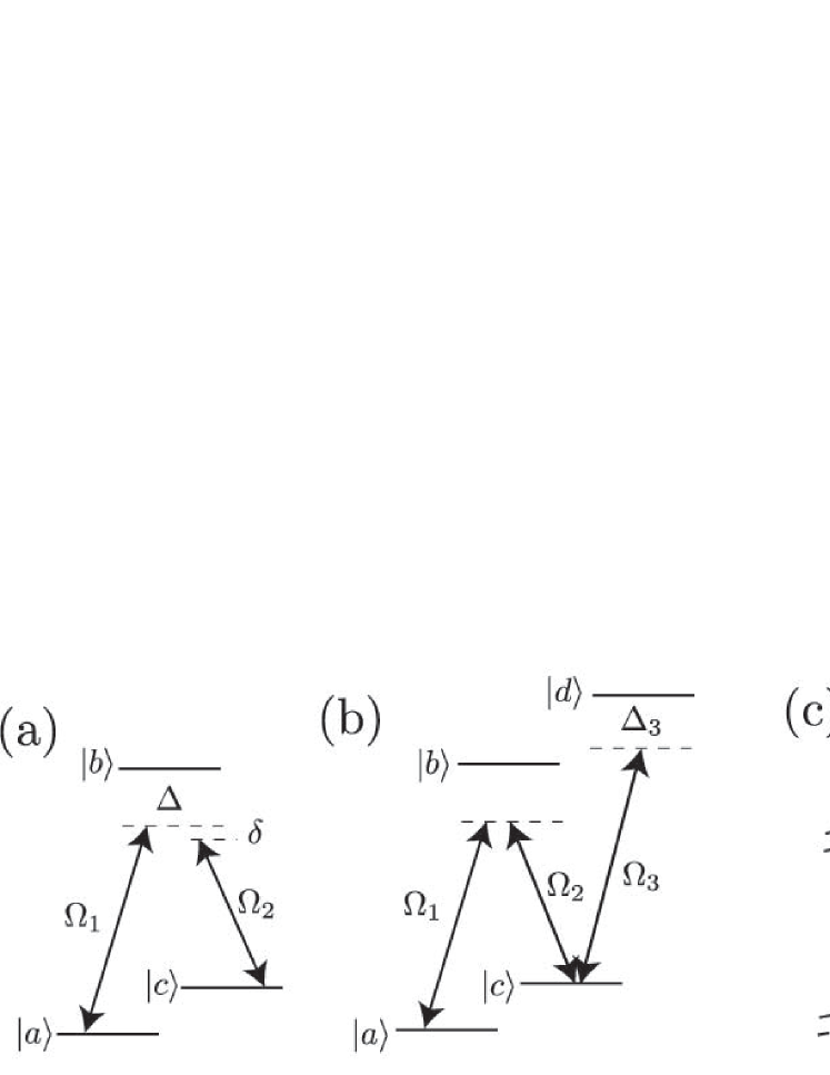
Figure 1: (a) Schematic of the three-state $\Lambda$ system under consideration. States $|a\rangle$ and $|c\rangle$ are ground (meta-stable) states, and have no direct spontaneous emission pathways. $|b\rangle$ is an excited state, which decays to $|a\rangle$ and $|c\rangle$ with equal probabilities. The $|a\rangle-|b\rangle$ transition is driven by field 1, with detuning $\Delta$ and Rabi frequency $\Omega_{1}$ (pump). The $|b\rangle-|c\rangle$ transition is driven by field 2 (probe) with detuning $\Delta+\delta$ (i.e. $\delta$ is the shift from the mutual detuning $\Delta$) and Rabi frequency $\Omega_{2}$. (b) Schematic of four-state system in the $N$ configuration, where the $\Lambda$ system is modified by an interaction with field 3 driving (off-resonantly) the $|c\rangle-|d\rangle$ transition with Rabi frequency $\Omega_{3}$ and detuning $\Delta_{3}$. To first order, we expect the $|c\rangle-|d\rangle$ transition to perturb the EIT in the $|a\rangle-|b\rangle-|c\rangle$ system via the usual light shift, which plays a role equivalent to the two-photon detuning in the three-state scheme. (c) Proposed configurations for realising the QND measurement. Fields 1 and 3 enter a single-mode diamond waveguide constructed from a photonic bandgap material with tailored group velocity for field 3 and of order $100~{}\mu\mathrm{m}$ long. Two illustrations of potential structures are shown, the lower follows Krauss [30], and the upper is via coupled cavity arrays in the style of Altug and Vučković [31] Field 2 (not shown) illuminates from the side. The unknown field, field 3, propagates unperturbed, but field 1 is phase shifted by the number of photons in field 3, and this phase shift can be read out using heterodyne methods (not shown).

EIT is a well-known mechanism for generating optical nonlinearities without loss [2], for a recent review see Ref. [32]. The typical (and minimal) system in which to observe EIT is a three-state system in the $\Lambda$ configuration with two driving fields, depicted in Fig. 1(a) with states labelled $|a\rangle$, $|b\rangle$ and $|c\rangle$. EIT is a manifestation of quantum interference in an atomic system: Considering field 1 as a ‘pump’ and field 2 as a ‘probe’, absorption of the probe is suppressed due to the coherence induced by the pump. The coherence gives rise to interference between the dressed states on the $|a\rangle-|b\rangle$ transition, and hence a dip in the probe absorption. Because the absorption dip is due to a coherent two-photon resonance (the resonant two-photon transition from $|a\rangle$ to $|c\rangle$) it can, in principle, be much less than the optical linewidth of the $|b\rangle-|c\rangle$ transition, limited only by the decoherence on the $|a\rangle-|c\rangle$ transition.

Although transparency is the eponymous feature of EIT, of more practical interest is the steep and controllable dispersion curve that is associated with the transparency point. A typical example of the dispersive and absorptive spectra associated with EIT are shown in Fig. 2. At the transparency point (two-photon resonance between the ground states) there is a linear dispersion. This feature has led to dramatic demonstrations of ultra-slow group velocity light [20, 34, 35] and is the basis for the Giant Kerr nonlinearity [33] in the $N$ configuration of Fig. 1 (b). Considering the $N$ system as a $\Lambda$ system perturbed by an off-resonant transition, one can see that the detuned off-resonant third field induces a small light shift to $|c\rangle$. Although this is a small effect, because of the steepness of the dispersion, a large effect on the EIT resonance is observed. This property was proposed for achieving photonic blockade in cavity QED systems [36], and has undergone extensive theoretical investigation (e.g. Refs. [37, 38, 39, 40, 41]) and recently observed [42] (although in the two-state, rather than four-state configuration). When field 3 is resonant, an absorptive, rather than dispersive, nonlinearity is observed, which has been studied theoretically [7] and experimentally [43, 44], and will not be treated here. Neither do we consider the many related atomic configurations, e.g. the Tripod [45], extended N [46], Chain-$\Lambda$ [47], and $M$-scheme [48], although they all offer potential improvements over the conventional $N$ scheme.

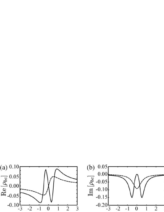
Figure 2: Typical dispersion (a) and absorption (b) curves associated with EIT in a $\Lambda$ system (solid lines) compared to those of a two-state system with equal probe couplings (dashed lines). The narrow EIT resonance is associated with linear dispersion at $\delta=0$. The steep slope makes it easy to perturb the EIT resonance and gives rise to the Giant Kerr effect.

One important detail for realising nonlinear interactions in the $N$ system is that of group velocity matching. In a travelling wave geometry to realise the $N$ system of Fig. 1 (b), we require the pulses that describe fields 1 and 3 to be temporally coincident for the maximum cross-Kerr interaction (the classical pump field 2 can be assumed to be derived from a large uniform field, and so is exempt from this criterion). Because field 1 is travelling under EIT conditions, it will be propagating with extremely slow group velocity: field 3 is not. We see that the amount of mutual interaction would therefore be expected to be limited by the temporal walk-off of the two pulses. There have been many suggestions in the literature to counter this effect (e.g. Refs. [49, 50]) which invoke varying levels of complexity of the interaction medium. It is also possible to control group velocity by modification of the medium, e.g. by using tailored photonic bandgap structures [51, 52]. Because we are mainly interested in solid-state implementations, we will assume that the system is embedded in a photonic-crystal structure where the group velocity as seen by field 3 is tuned by the structure to balance the EIT induced group velocity seen by field 1, and we therefore will not treat this detail further.

Although much of our treatment in this paper will be system independent, it is important to note that a major motivation for performing this reappraisal of weak nonlinear gates is the availability of a new material for observing optical EIT: diamond containing the negatively charged Nitrogen-Vacancy colour centre (NV). This material has shown quite remarkable results, including single photon generation (e.g. [53]), room-temperature Rabi oscillations [54], and spin-spin coupling [55, 56, 57, 58]. EIT has been demonstrated in NV diamond in the rf [13] and optical regimes [16, 17]. The intrinsic properties of NV centres can also be modified by fabricating optical structures directly in ultra-nanocrystalline [59] or single crystal diamond [60, 61, 62], by growth on preexisting optical structures [63], and also by Stark shifting which has been demonstrated on bulk samples [64] and spectrally resolved centres [65, 66]. The time is therefore ripe to examine NV diamond for the goal of optical quantum information processing.

In the next section, we discuss EIT and the properties of coherently driven $\Lambda$ systems. By including inhomogeneous broadening and expanding about the EIT point we are able to derive analytical results for the absorption and dispersion without the usual assumption of weak probe and strong pump fields. We are also able to determine optimal ratios for pump and probe Rabi frequencies. In Section 3 we show the results for cross-Kerr nonlinearities in the four-state N system, and in Section 4 we present our main results, which use the results from the preceeding sections to design structures based on diamond containing the Nitrogen-Vacancy colour centre that should be sufficient to realise a number-discriminating Quantum Non-Demolition operation.

2 Three-state $\Lambda$ system

A schematic of our model three-state system is shown in Fig. 1. Following Shore [67], we write down the Hamiltonian under the rotating wave approximation in matrix form with state ordering $|a\rangle,|b\rangle,|c\rangle$

$$\mathcal{H}=\hbar\left(\Delta\sigma_{bb}+\delta\sigma_{cc}+\Omega_{1}\sigma_{ba}+\Omega_{2}\sigma_{cb}+h.c.\right),$$ (1)

where field 1 (field 2) drives the $|a\rangle-|b\rangle$ ($|b\rangle-|c\rangle$) transition with Rabi frequency $\Omega_{1}$ ($\Omega_{2}$) and detuning $\Delta_{1}$ ($\Delta_{2}$), and $\sigma_{ij}=|i\rangle\langle j|$. As we are operating near the two-photon resonance, we set $\Delta_{1}=\Delta$ and $\Delta_{2}=\Delta+\delta$ where $\Delta$ is the mutual detuning, and $\delta$ is the detuning from two-photon resonance. Spontaneous emission at rate $\Gamma$ is from $|b\rangle$ to $|a\rangle$ and $|c\rangle$ with equal probabilities. We treat inhomogeneous broadening by considering a distribution of $\Delta$, i.e. the mutual detunings. As we are only considering inhomogeneity on the excited state distribution, the two-photon detuning, $\delta$, does not vary. Note that although we will use terminology such as ‘pump’ and ‘probe’, we will usually make no assumption about the relative strength of these fields. In this way our analysis is analogous to the cases treated by Wielandy and Gaeta on EIT in the strong pump regime [68] or the parametric EIT regime [69].

One way to proceed in gaining insight on the EIT problem set out in Eq. 1 is to construct the master equation and determine the steady state solution. This can be expressed as

$$\dot{\rho}=-\frac{i}{\hbar}[\mathcal{H},\rho]+\sum_{j}\Gamma_{j}\mathcal{L}[B_{j},\rho],$$ (2)

where we have introduced the usual density matrix, $\rho$ and the Liouvillian super-operator, $\mathcal{L}[B,\rho]$ which describes the effect of the generalised decoherence channel $B$ with rate $\Gamma\geq 0$ on the density matrix, and is summed over all decoherence channels. The Liouvillian operators are defined

$$\mathcal{L}[B,\rho]\equiv B\rho B^{{\dagger}}-\frac{1}{2}\left(B^{{\dagger}}B\rho+\rho B^{{\dagger}}B\right).$$ (3)

In our case,we restrict ourselves to the case that the system is limited by spontaneous emission, and that the decoherence between the ground states can be neglected. This approximation is warranted because of the very long ground state decoherence rates in important systems of interest (e.g. diamond containing the negatively charged Nitrogen-Vacancy colour centre [56], or rubidium vapour cells [34]) but does limit the minimum Rabi frequencies that can be applied to be larger than this decoherence rate. So here, the $B$ will be the one-way (spontaneous emission) transitions from $|b\rangle$ to either $|a\rangle$ ($\sigma_{ab}$) or $|c\rangle$ ($\sigma_{cb}$) with rate, $\Gamma/2$.

To analyse Eq. 2 in the steady state, we convert the master equation into superoperator form, and write

$$\dot{\vec{\rho}}=\left(-i\mathcal{P}+\mathcal{L}\right)\vec{\rho},$$ (4)

where $\vec{\rho}$ is the vector obtained by writing out the density matrix elements, and $\mathcal{P}$ and $\mathcal{L}$ are the superoperators describing Hamiltonian and decoherence processes respectively.

In addition to the master equations, we also include the effect of inhomogeneous broadening. Inhomogeneous broadening has been treated previously in the context of Doppler-broadened EIT in vapour cells (e.g. [70, 71]), and is treated as a Gaussian distribution of the absolute energy of $|b\rangle$, which in turn is manifested as a variation in $\Delta$ across the sample, i.e. there is a probability distribution of detunings

$$P(\Delta)=\frac{1}{\sqrt{2\pi\gamma^{2}}}\exp\left[-\frac{\left(\Delta-\Delta_{0}\right)^{2}}{2\gamma^{2}}\right],$$ (5)

where $\Delta_{0}=\int_{-\infty}^{\infty}\Delta P(\Delta)d\Delta$ is the mean mutual detuning with respect to the inhomogeneous linewidth, which has standard deviation $\gamma$. Fig. 3 shows spectra with the real and imaginary parts of the $|b\rangle-|c\rangle$ coherence, $\rho_{bc}$ (proportional to the probe dispersion and absorption respectively) with $\Omega_{1}=\Gamma/2$ and $\Omega_{2}=\Gamma/10$ to illustrate the effect of inhomogeneous broadening on the resonant EIT profile. Figs. 3 (a) and (b) show the absorption and dispersion curves for $\Delta$ from 0 to positive values showing the effect of increasing $\Delta$. Note that spectra of the same colour go together. Although the overall spectra are quite different, in the vicinity $\delta=0$ they are all locally similar. This is clearer in Figs. 3 (c) and (d) which shows spectra from large negative to positive $\Delta$ superimposed, showing the local similarity strongly. Figs. 3 (e) and (f) show the effect over the whole inhomogeneous linewidth with $\gamma=10\Gamma$ (solid blue line) compared with the a sample with equal total population but only homogeneously broadened sample (black dashed line). Note that these plots may equally well be interpreted as classic hole-burning spectra [72]. The self-similarity of the EIT traces is not dependent upon the mutual detuning, as is illustrated in Fig. 4 which compares $\Delta_{0}=0$ with $\Delta_{0}=-\Gamma$.

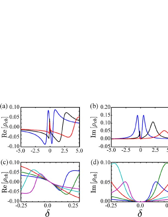
Figure 3: EIT in for homogeneously broadened systems. (a) $\mathrm{Re}(\rho_{cb})$ as function of $\delta$ for the mutual detunings of $\Delta=0,~{}2\Gamma,~{}4\Gamma$ (blue, black and red lines respectively) to illustrate the effect of moving away from resonance. (b) Absorption [$\mathrm{Im}(\rho_{cb}$] under the same conditions. Again note that all of the EIT transparency windows overlap. (c) Closeup in the vicinity of $\delta=0$, showing $\mathrm{Re}(\rho_{cb})$ this time for $\Delta=-2\Gamma,~{}-\Gamma,~{}0,~{}\Gamma,~{}2\Gamma$ (blue, green, red, cyan and magenta lines respectively) (d) Analogous spectra for $\mathrm{Im}(\rho_{cb})$.

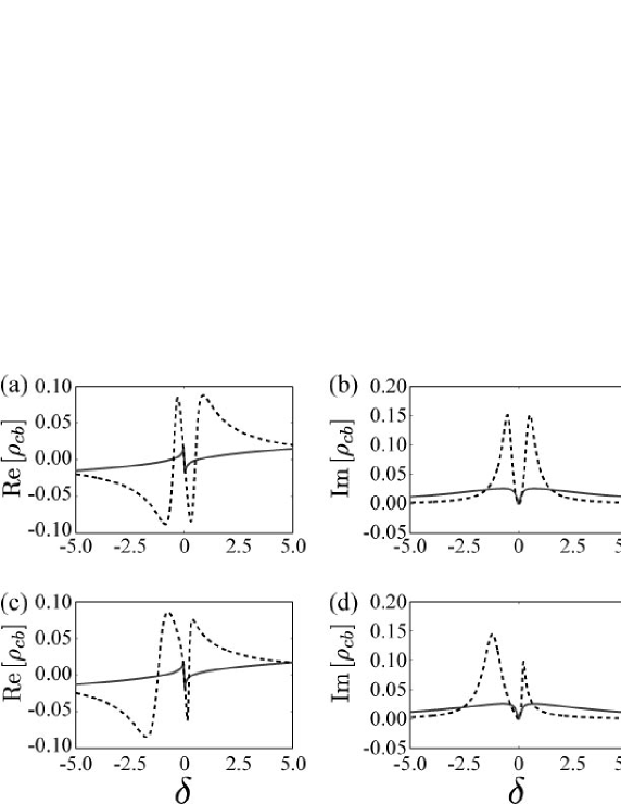
Figure 4: Comparison of EIT traces as a function of the detuning from the two-photon resonance condition, $\delta$, for one-photon resonance, (a) real part, (b) imaginary part, and finite mutual detuning, $\Delta=2\Omega$, (c) real part and (d) imaginary part. In each case the dashed line is the single-atom result, whilst the solid lines are the average over the inhomogeneous line, with $\gamma=10\Gamma$. Although the overall lineshapes vary with $\Delta$ and inhomogeneity, the $\delta=0$ responses are equivalent to second order.

The self-similarity of the EIT profiles about $\delta=0$ may be understood by considering $\rho_{bc}$ in the steady state. Setting $\dot{\vec{\rho}}=0$, we determine the null-space which gives the non-trivial steady state solution for $\vec{\rho}^{(ss)}$. In general the analytical results are somewhat complicated. By confining our interest to the region around $\delta=0$, i.e. in the vicinity of the two-photon resonance, we may perform a series solution for $\vec{\rho}^{(ss)}$ in powers of $\delta$, which yields to first order

$$\rho_{aa}=\frac{\Omega_{2}^{2}}{\Omega_{1}^{2}+\Omega_{2}^{2}}-\frac{2\Omega_{1}^{2}\Omega_{2}^{2}\Delta}{\left(\Omega_{1}^{2}+\Omega_{2}^{2}\right)^{3}}\delta,$$ (6)

$$\rho_{ab}=\frac{\Omega_{1}\Omega_{2}^{2}}{\left(\Omega_{1}^{2}+\Omega_{2}^{2}\right)^{2}}\delta=\rho_{ba}^{\ast},$$ (7)

$$\rho_{ac}=-\frac{\Omega_{1}\Omega_{2}}{\Omega_{1}^{2}+\Omega_{2}^{2}}+\frac{\Omega_{1}\Omega_{2}\left[\Delta\left(\Omega_{1}^{2}-\Omega_{2}^{2}\right)-i\Gamma\left(\Omega_{1}^{2}+\Omega_{2}^{2}\right)\right]}{\left(\Omega_{1}^{2}+\Omega_{2}^{2}\right)^{3}}\delta=\rho_{ca}^{\ast},$$ (8)

$$\rho_{bb}=0,$$ (9)

$$\rho_{cb}=-\frac{\Omega_{1}^{2}\Omega_{2}}{\left(\Omega_{1}^{2}+\Omega_{2}^{2}\right)^{2}}\delta=\rho_{bc}^{\ast},$$ (10)

$$\rho_{cc}=\frac{\Omega_{1}^{2}}{\Omega_{1}^{2}+\Omega_{2}^{2}}+\frac{2\Omega_{1}^{2}\Omega_{2}^{2}\Delta}{\left(\Omega_{1}^{2}+\Omega_{2}^{2}\right)^{3}}\delta.$$ (11)

Cursory inspection of these steady state results provides some very important properties of the EIT condition. Modelling of inhomogenous broadening was to be by varying $\Delta$ over the ensemble, however assuming field 1 is the pump and field 2 the probe, then the parameter of interest for EIT is $\rho_{cb}$. From the above, we see the well-known linear dependance with detuning expected for an EIT resonance, which has no dependence on $\Delta$, indicating that inhomogeneous broadening will affect neither the absorption nor dispersion seen by the probe field to first order in the probe detuning (but to all orders in the mutual detuning). This is an important result, highlighting that EIT is extremely robust to inhomogeneous broadening in the excited state. To see effects due to the inhomogenous broadening of the line, we will need to go to higher orders in $\delta$.

The total coherence is obtained by integrating over the inhomogeneous linewidth, so we have

$$\varrho_{cb}=\int_{-\infty}^{\infty}P(\Delta)\rho_{cb}~{}d\Delta,$$ (12)

where we have introduced $\varrho_{cb}$ as the coherence integrated over the inhomogeneous line. As $\int_{-\infty}^{\infty}P(\Delta)d\Delta=1$, to first order in $\delta$, we have trivially that $\varrho_{cb}=\rho_{cb}$. To see effects due to the inhomogeneous line, we must go to second order in $\delta$, where we have

$$\rho_{cb}^{(2)}=\frac{\Omega_{1}^{2}\Omega_{2}}{(\Omega_{1}^{2}+\Omega_{2}^{2})^{2}}\left[-\delta+\frac{\left(\Omega_{1}^{2}-3\Omega_{2}^{2}\right)\Delta\delta^{2}}{(\Omega_{1}^{2}+\Omega_{2}^{2})^{2}}+i\frac{\Gamma\delta^{2}}{(\Omega_{1}^{2}+\Omega_{2}^{2})}\right]+\mathcal{O}[\delta]^{3}.$$

(13)

Performing the integration over the inhomogeneous line yields

$$\varrho_{cb}^{(2)} = \int_{-\infty}^{\infty}P(\Delta)\rho_{cb}^{(2)}d\Delta,$$ (14)

$$= \frac{\Omega_{1}^{2}\Omega_{2}}{(\Omega_{1}^{2}+\Omega_{2}^{2})^{2}}\left[-\delta+\frac{\left(\Omega_{1}^{2}-3\Omega_{2}^{2}\right)\Delta_{0}\delta^{2}}{(\Omega_{1}^{2}+\Omega_{2}^{2})^{2}}+i\frac{\Gamma\delta^{2}}{(\Omega_{1}^{2}+\Omega_{2}^{2})}\right].$$ (15)

Regions with high dispersion are associated with regions of high nonlinearity, and hence will inform us in our search for optimal working points for our gates. The probe dispersion is defined

$$R_{cb}\equiv\frac{\partial\mathrm{Re}[\rho_{cb}]}{\partial\delta},$$ (16)

and using the first order solution in eq. 10 we obtain

$$R_{cb}=-\frac{\Omega_{1}^{2}\Omega_{2}}{\left(\Omega_{1}^{2}+\Omega_{2}^{2}\right)^{2}}.$$ (17)

Note that if we set $\Omega_{1}=\sqrt{3}\Omega_{2}$, then the second order correction to the refractive index in Eq. 13 is nulled, and we must therefore go to third order in $\delta$ (or higher) to observe terms depending explicitly on the inhomogeneous broadening. This result also carries through to the dispersion, i.e. that the gradient is largest when $\Omega_{1}$ and $\Omega_{2}$ are smallest and maximised when $\Omega_{1}=\sqrt{3}\Omega_{2}$. A graph showing $\log_{10}(-R)$ as a function of $\Omega_{1}$ and $\Omega_{2}$ is shown in Fig. 5, along with a line showing the maximal dispersion at $\Omega_{1}=\sqrt{3}\Omega_{2}$. These results may be useful to optimise slow and stopped light experiments, however for the purposes of QND measurements (as will be seen in Section 4) the susceptibility is simply maximised for minimum possible $\Omega_{1}$.

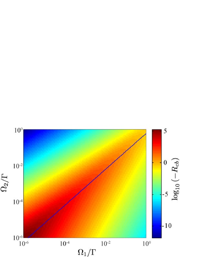
Figure 5: First order probe dispersion, plotted as $\log_{10}(-R_{cb})$ as a function of $\Omega_{1}$ (pump) and $\Omega_{2}$ (probe) in the vicinity of two-photon resonance in a three-state system. Note that the dispersion as seen by the probe will be largest when $\Omega_{1}=\sqrt{3}\Omega_{2}$, and goes as $R_{cb}=-3\sqrt{3}/(16\Omega_{1})$ in this limit. This optimal solution for $R$ is indicated by the solid line.

To explore the absorption we take the imaginary part of the solution for $\rho_{cb}$, which is to third order in $\delta$

$$A=\frac{\Omega_{1}^{2}\Omega_{2}\Gamma}{(\Omega_{1}^{2}+\Omega_{2}^{2})^{3}}\delta^{2}-2\Delta\Gamma\frac{\Omega_{1}^{2}\Omega_{2}(\Omega_{1}^{2}-\Omega_{2}^{2})}{(\Omega_{1}^{2}+\Omega_{2}^{2})^{5}}\delta^{3}+\mathcal{O}[\delta^{4}].$$ (18)

Ignoring the third order correction, here we see the familiar quadratic dependance with respect to detuning, and as presaged above, there is no contribution to the absorption from $\Delta$. We can infer the bandwidth of the EIT medium, by considering the effect of the EIT window on a pulse with finite bandwidth. Fig. 6(a) shows schematically a transform limited Gaussian pulse propagating through the quadratic EIT window. If we assume that the pulse is defined by some spectral width $f$, centered around the EIT window at $\delta=0$, with the functional form $\exp[-\delta^{2}/(2f^{2})]/\sqrt{2\pi f^{2}}$, then to determine the total (single atom) absorption we integrate the pulse over the EIT window, i.e.

$$\mathcal{A} = \int_{-\infty}^{\infty}\frac{\exp\left[-\delta^{2}/(2f^{2})\right]}{\sqrt{2\pi f^{2}}}\frac{\Omega_{1}^{2}\Omega_{2}\Gamma}{(\Omega_{1}^{2}+\Omega_{2}^{2})^{3}}\delta^{2}d\delta,$$ (19)

$$= \frac{\Omega_{1}^{2}\Omega_{2}\Gamma f^{2}}{(\Omega_{1}^{2}+\Omega_{2}^{2})^{3}},$$ (20)

and this quantity will prove essential in determining bandwidth requirements in the design of practical nonlinear gates. To explore this, we calculate in Fig. 6(b) the bandwidth in units of the spontaneous emission, $f/\Gamma$ as a function of $\Omega_{1}/\Gamma$ and $\Omega_{2}/\Gamma$ that will achieve a $\mathcal{A}=1\%$. Such analyses as these allow us to determine gate speeds for QND measurements and will be exploited in Section 4.

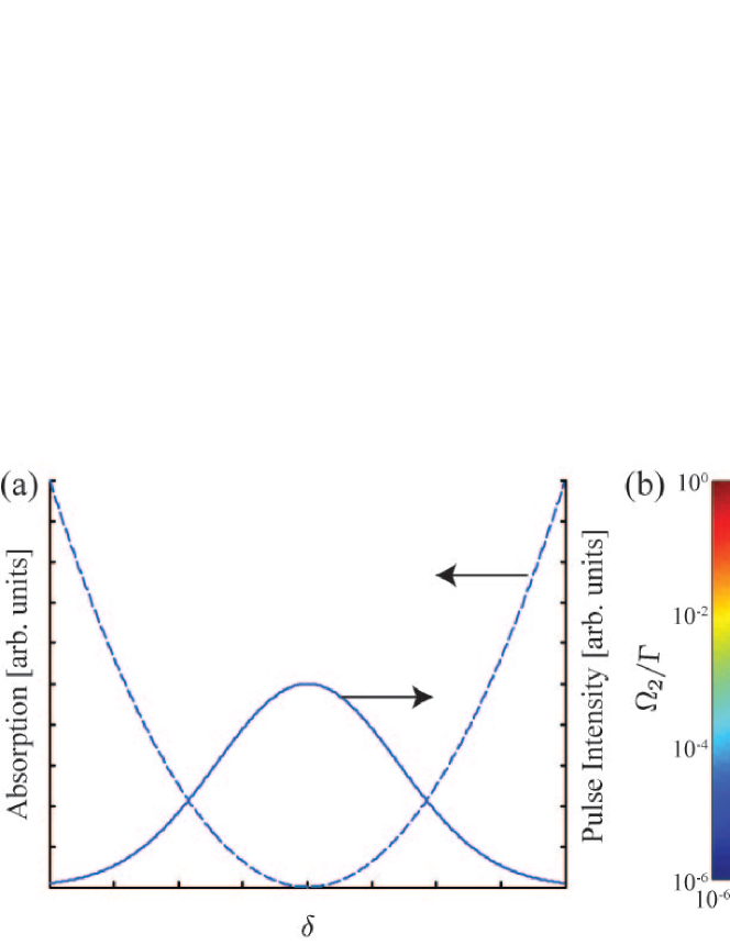
Figure 6: (a) Schematic showing the absorption seen by an optical pulse with finite bandwidth. To second order, the EIT window has absorption that is quadratic in $\delta$, where a transform limited pulse is a Gaussian in $\delta$, so the residual absorption per unit length seen by a pulse travelling through an EIT window will be found by taking the overlap integral of the pulse and absorption. (b) Log base 10 of the maximum bandwidth in units of $\Gamma$ that will attain $\mathcal{A}=1\%$ as a function of $\Omega_{1}/\Gamma$ and $\Omega_{2}/\Gamma$. Note that although the bandwidths can be quite small, they are still of order the Rabi frequencies of the fields, which accords with our intuition about the width of the EIT window. The smallest allowable bandwidth coincides with the largest dispersions, again as one would expect.

Finally, we comment on the group velocity seen under conditions of EIT. Group velocity reduction is one of the most dramatic consequences of EIT and is observable in the usual pump-probe arrangement (e.g. [20, 34]). Perhaps surprisingly, large changes in the group velocity between fields (group velocity mismatch) can actually lead to a strong reduction in effective coupling. As mentioned previously, we propose group velocity engineering as the solution to this mismatch, but it is essential to understand the group velocity under conditions of EIT in order to specify the propagation properties of the unknown field.

The group velocity of a probe field can be determined using Eq. 17, so we have

$$v_{g_{ab}} = \frac{c}{\eta+\frac{\omega_{1}}{2}\frac{\partial\chi_{ab}}{\partial\Delta}},$$ (21)

where $\eta$ is the bulk refractive index, and we have introduced the susceptibility

$$\chi_{ab}=\frac{2\pi\mathcal{N}}{\varepsilon_{0}\varepsilon_{R}\hbar}\frac{\mu_{ab}^{2}}{\Omega_{1}}\rho_{ab},$$ (23)

and so

$$\frac{\partial\chi_{ab}}{\partial\delta} = \frac{2\pi\mathcal{N}}{\varepsilon_{0}\varepsilon_{R}\hbar}\frac{\mu_{ab}^{2}}{\Omega_{1}}R_{ab},$$ (24)

$$= \frac{2\pi\mathcal{N}}{\varepsilon_{0}\varepsilon_{R}\hbar}\mu_{ab}^{2}\frac{\Omega_{2}^{2}}{\left(\Omega_{1}^{2}+\Omega_{2}^{2}\right)^{2}},$$ (25)

where $\mathcal{N}$ is the number density of atoms. So in the limit that the group velocity reduction is large, we have

$$v_{g_{ab}}=\frac{c\varepsilon_{0}\varepsilon_{R}\hbar}{\pi\omega\mathcal{N}\mu_{ab}^{2}}\frac{\left(\Omega_{1}^{2}+\Omega_{2}^{2}\right)^{2}}{\Omega_{2}^{2}}.$$ (26)

Ultimately we will be interested in the group velocity associated with quantised fields, rather than the semiclassical form above. Making the substitution $\tilde{\Omega}_{1}\sqrt{n_{1}}=\Omega_{1}$ where $n_{1}$ is the number of photons in the mode, gives the group velocity seen by a mode with $n_{1}$ photons of

$$v_{g_{ab}}=\frac{c\varepsilon_{0}\varepsilon_{R}\hbar}{\pi\omega\mathcal{N}\mu_{ab}^{2}}\frac{\left(\tilde{\Omega}_{1}^{2}n_{1}+\Omega_{2}^{2}\right)^{2}}{\Omega_{2}^{2}}.$$ (27)

These results will be used in Section 4, especially with quantisation of the probe field. In general one would seek the largest possible $v_{g}$ that enables effective coupling, so as to minimise the reduction in the group velocity on the unknown signal which is not travelling under conditions of EIT reduced group velocity. Also the group velocity dispersion which will manifest with uncertainty in the number of photons in the probe field is also a potential source of error and should be minimsed. This implies a rule of thumb, that we should seek operation in the limit of large $n_{1}$ to minimise the relative variation in $v_{g}$.

3 Four-state $N$ system

The four-state $N$ scheme is one level structure that clearly shows a cross-Kerr effect, and is illustrated in Fig. 1(b). There is much freedom to choose which fields correspond to pump, probe and driving, and all appear to have been treated in the literature in various places. For concreteness, we will treat the $N$ system as a $\Lambda$ perturbed by an off-resonant transition. Furthermore, we will be considering the effect of the $|b\rangle-|d\rangle$ transition (hence field 3) on field 1, so in this section, the parameters of interest will be $\rho_{ab}$ and $\varrho_{ab}$. For this case we set the operating point for the $\Lambda$ system as $\delta=0$. Under these conditions, the Hamiltonian is

$$\mathcal{H}=\hbar\left(\Delta\sigma_{bb}+\Delta_{3}\sigma_{dd}+\Omega_{1}\sigma_{ba}+\Omega_{2}\sigma_{cb}+\Omega_{3}\sigma_{dc}+h.c.\right),$$ (28)

where the (in general unknown) Rabi frequency of field 3 is $\Omega_{3}$ and it is detuned from the $|b\rangle-|d\rangle$ transition by $\Delta_{3}\gg\Omega_{3}$.

In the case that the $|c\rangle-|d\rangle$ transition is only homogenously broadened, we may treat the effect of field 3 on the $|a\rangle-|b\rangle-|c\rangle$ system quite simply. Our treatment here follows and extends Ref. [8]. The effect of a field 3 on the $|c\rangle-|d\rangle$ transition can be seen as an off-resonant light-shift, which in turn perturbs the $|a\rangle-|b\rangle-|c\rangle$ $\Lambda$ EIT. The strength of the light shift can be directly equated with the $-\delta$ (the shift will be in the opposite direction) from the previous analysis, i.e.

$$\delta=-\frac{\Omega_{3}^{2}}{\Delta_{3}},$$ (29)

in the limit that $\Delta_{3}\gg\Omega_{3}$. Recalling that the residual population in $|d\rangle$ is a source of error, we will assume that this population must be kept below some threshold, $\epsilon$, i.e.

$$\rho_{dd}=\left(\frac{\Omega_{3}}{\Delta_{3}}\right)^{2}\leq\epsilon.$$ (30)

Using the previous result for the steady state of $\rho_{ab}$, and substituting for $\delta$, we have

$$\rho_{ab}=-\frac{\Omega_{1}\Omega_{2}^{2}}{\left(\Omega_{1}^{2}+\Omega_{2}^{2}\right)^{2}}\frac{\Omega_{3}^{2}}{\Delta_{3}}.$$ (31)

The Hamiltonian of Eq. 28 can also be attacked using the superoperator approach. We assume that all decay from $|d\rangle$ is to $|c\rangle$ at rate $\Gamma$, and keeping the other terms the same from the $\Lambda$ analysis, except $\Delta=0$. We can obtain the steady state response quite easily, but for clarity, we only report the coherence on the $|a\rangle-|b\rangle$ transition, which is

$$\rho_{ab}=-\frac{2\Omega_{1}\Omega_{2}^{2}\Omega_{3}^{2}}{(2\Delta_{3}+i\Gamma)(\Omega_{1}^{2}+\Omega_{2}^{2})^{2}}+\mathcal{O}[\Omega_{3}]^{4},$$ (32)

which is qualitatively very similar to the previous result, but with the inclusion of an extra absorption term.

To move to the case of a finite inhomogeneous linewidth, we first recall that we may safely ignore linewidth to first order on the $\Lambda$ system, however, we cannot do so on the $|b\rangle-|d\rangle$ transition, as $\Delta_{3}$ appears directly in the coherence. Therefore, using the light-shifted treatment from Eq. 31 we write down the ensemble coherence as

$$\varrho_{ab} = \int_{-\infty}^{\infty}P(\Delta_{3})\rho_{ab}d\Delta_{3},$$ (33)

$$= -\frac{\Omega_{1}\Omega_{2}^{2}\Omega_{3}^{2}}{\sqrt{2\pi\gamma^{2}}\left(\Omega_{1}^{2}+\Omega_{2}^{2}\right)^{2}}\int_{-\infty}^{\infty}\frac{\exp[-(\Delta_{3}-\Delta_{0})^{2}/(2\gamma^{2})]}{\Delta_{3}}d\Delta_{3},$$ (34)

$$= -\frac{\sqrt{\pi}\Omega_{1}\Omega_{2}^{2}\Omega_{3}^{2}}{\sqrt{2\gamma^{2}}\left(\Omega_{1}^{2}+\Omega_{2}^{2}\right)^{2}}\exp\left(-\frac{\Delta_{0}^{2}}{2\gamma^{2}}\right){\rm erfi}\left(\frac{\Delta_{0}}{\sqrt{2\gamma^{2}}}\right),$$ (35)

where ${\rm erfi}(x)={\rm erf}(ix)/i$ is the imaginary error function. Note that although we have treated the inhomogeneous linewidths for $|d\rangle$ as equivalent to that of $|b\rangle$, the analysis is practically unchanged if we took a more general case. It is instructive to examine the behaviour of just the exponential and imaginary error function terms, to determine the optimal ratio of mean detuning to inhomogeneous linewidth. Setting $d=\Delta_{0}/\sqrt{2\gamma^{2}}$ as the mean detuning in units of the linewidth, and $J(d)\equiv\exp(-d^{2}){\rm erfi}(d)$ in Fig. 7 we plot $J(d)$ vs $d$, as for constant $\gamma$, all the other terms are constant. The maximum of $J$ can be seen as being just before $d=1$, however, care must be taken in this limit, and there will still be appreciable absorption of field 3 in this limit (as there will be on-resonant atoms). However, detuning by 5 inhomogenous linewidths (i.e. $d=5$) only has the effect of reducing the effective $\varrho_{ab}$ by about one sixth compared to a homogeneously broadened sample at such a detuning: the larger effect is the penalty in having to go to such large detunings to avoid the line (i.e. for a homogenously broadened sample, one could work closer to resonance).

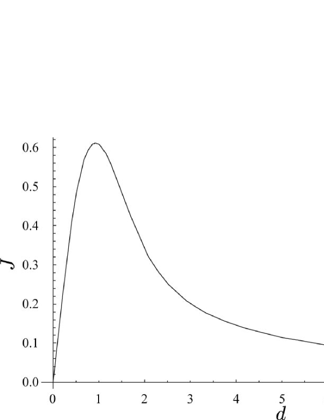
Figure 7: Graph showing optimal mean detuning from resonance in units of the inhomogeneous linewidth. Here we have taken our figure of merit to be $J(d)\equiv\exp(-d^{2}){\rm erfi}(d)$ which is the term in $\varrho_{ab}$ which depends explicitly on $d=\bar{\Delta}/(2\gamma)$. Note that the results for $d\lesssim 1$ will not be relevant for our discussion because the condition $\Omega_{3}\ll\Delta_{3}$ may be unsatisfied, and there may also be significant resonant one-photon absorptions of field 3

An alternative transition to be considered for the readout is the $|c\rangle-|d\rangle$ transition. The coherence associated with this can also be determined and is

$$\rho_{cd}=-\frac{2\Omega_{1}^{2}\Omega_{3}}{(2\Delta_{3}+i\Gamma)(\Omega_{1}^{2}+\Omega_{2}^{2})}+\mathcal{O}[\Omega_{3}]^{3}.$$ (36)

Integrating this over the inhomogeneity on the $|c\rangle-|d\rangle$ transition does not yield analytic solutions, however by replacing the denominator by the large detuning approximation (i.e. the term $(2\Delta_{3}+i\Gamma)/2$ is replaced by $\Delta_{3}$, we get

$$\varrho_{cd}=-\frac{\sqrt{\pi}\Omega_{1}^{2}\Omega_{3}}{\sqrt{2\gamma^{2}}(\Omega_{1}^{2}+\Omega_{2}^{2})}\exp\left(-\frac{\Delta_{0}}{2\gamma^{2}}\right)\textrm{erfi}\left(\frac{\Delta_{0}}{\sqrt{2\gamma^{2}}}\right).$$ (37)

For completeness, we also report the coherence on the $|c\rangle-|b\rangle$ transition, which is

$$\rho_{cb}=\frac{2\Omega_{1}^{2}\Omega_{2}\Omega_{3}^{2}}{(2\Delta_{3}-i\Gamma)(\Omega_{1}^{2}+\Omega_{2}^{2})^{2}}.$$ (38)

As the response here is clearly analogous to that of $\rho_{ab}$ we will not repeat any further discussion of using this transition for monitoring any probe state, except to note that changing between $|a\rangle-|b\rangle$ and $|c\rangle-|b\rangle$ may perhaps be useful for reasons of experimental convenience in certain implementations, but otherwise would appear to hold no benefits.

It is interesting to note that neither Eq. 32 nor 36 exhibit self-Kerr effects, with the first self nonlinearities for $\rho_{ab}$ appearing at fourth order, and for $\rho_{cd}$ appearing at third order. The presence of Kerr terms would hamper state discrimination in nonlinear gates (see next section) [73, 74]. One should note that the canonical method for generating self-Kerr terms in EIT media is to allow a field to interact with more than one transition (e.g. [36, 46, 47]) which effectively converts the cross-Kerr nonlinearity into a self-Kerr nonlinearity. The suppression of self-Kerr terms is desirable, as they give rise to pulse distortion which can limit the effectiveness of any gate based on nonlinear interactions.

Finally, we comment further on the populations in the excited states. In Eq. 30 we presented a simple two state argument for the population in state $|d\rangle$, which was viewed as a potential source of error. We now examine the full solutions for $\rho_{bb}$ and $\rho_{dd}$, which turn out to be qualitatively similar to the analysis based on perturbing the EIT structure by the extra transition.

Starting with $\rho_{dd}$, we find that the expansion to third order in $\Omega_{3}$ yields

$$\rho_{dd}=\frac{\Omega_{1}^{2}}{\Omega_{1}^{2}+\Omega_{2}^{2}}\frac{\Omega_{3}^{2}}{\Delta_{3}^{2}+(\Gamma/2)^{2}}+\mathcal{O}[\Omega_{3}]^{4}$$ (39)

This result can be immediately interpreted as the usual, off-resonant population from Eq. 30 (with spontaneous emission explicitly included), scaled by a factor due to the diminished population in $|c\rangle$ because of the coherent population trapping in the $\Lambda$ system. Similarly we can calculate the population in $|b\rangle$. Although the unperturbed EIT condition leads to no steady-state population in $|b\rangle$, the perturbed EIT will give rise to non-zero population. As above, this can be calculated and to third order in $\Omega_{3}$ we obtain

$$\rho_{bb}=\frac{\Omega_{1}^{2}\Omega_{2}^{2}}{(\Omega_{1}^{2}+\Omega_{2}^{2})^{2}}\frac{\Omega_{3}^{2}}{\Delta_{3}^{2}+(\Gamma/2)^{2}}+\mathcal{O}[\Omega_{3}]^{4}.$$ (40)

In general, if we have $\Omega_{2}=\sqrt{z}\Omega_{1}$, then we will have

$$\rho_{bb}=\frac{z}{(z+1)^{2}}\frac{\Omega_{3}^{2}}{\Delta_{3}^{2}+(\Gamma/2)^{2}},$$ (41)

$$\rho_{dd}=\frac{1}{z+1}\frac{\Omega_{3}^{2}}{\Delta_{3}^{2}+(\Gamma/2)^{2}}.$$ (42)

Any population occupying the excited states will in general be available for decoherence and give rise to errors. By inspection of Eqs. 41 and 42 we observe qualitatively the same familiar criterion from Eq. 30 (with minor corrections).

4 Implications for the design of QND weak nonlinear detectors

Our focus is on the construction of a device capable of achieving a QND measurement of the number of photons in a weak field. In this section we will combine the previous analyses above with realistic parameters that are achievable using a solid-state slow-light EIT waveguide, which contrasts with the more general discussion of EIT based nonlinear interactions. Our analysis focusses on QND measurement of a weak field with unknown photon number and we show discrimination between 0, 1 and 2 photons in the unknown field. In some of the parameter ranges discussed below, we also observe distortions of the probe field. Whilst this is not a problem for QND discrimination, it may restrict the utility of our discriminator for use in quantum gates [25], where the requirement for sequential use of the QND probe favours regimes where the Q-function of the probe is only rotated, and not also distorted by the nonlinear interaction.

We will first describe the appropriate metrics for evaluating the performance of any such gate in a material independent fashion, and then conclude by presenting realistic operating conditions in several potential implementations as a guide for future demonstrations. For clarity, throughout this section we will restrict ourselves to the case that the $|a\rangle-|b\rangle$ transition is probed by a weak coherent state, and the $|c\rangle-|d\rangle$ transition has the unknown signal field.

One of the most important parameters to determine the strength of the measurement signal is the effective Rabi frequency of the unknown pulse. Analysis of this will show that spatially confined structures (e.g. waveguides) will have a considerable advantage over free-space implementations. Following [75] we may express the single-photon Rabi frequency as

$$\tilde{\Omega}_{3}=\frac{\lambda_{12}}{4\pi}\sqrt{3\Gamma f\mathcal{N}l}$$ (43)

where we have introduced $\lambda_{12}$, the resonant transition free-space wavelength, $l$ the length of the medium (or with imperfect group velocity matching it will be the length of the effective interaction region) and recall that $f$ is the bandwidth of the single-photon pulse. The Rabi frequency is then

$$\Omega_{3}=\tilde{\Omega}_{3}\sqrt{n_{3}},$$ (44)

and the other Rabi frequencies can be defined similarly. Note that there is usually a dependence on the beam waist in Eq. 43, however this is compensated by the number of interacting four-state systems within the single photon spot size (so a larger spot interacts with more systems but with less strength). However, waveguide structures will still have significant advantages in minimising the beam cross-sectional area compared with free-space structures, with the effective medium length in free-space being ultimately limited by the Rayleigh range of the beam.

We first need to connect the microscopic description presented above with the macroscopically observable quantities. In particular, when considering the four-state system with the probe field on the $|i\rangle-|j\rangle$ transition, the phase shift seen by the probe [75]

$$K_{ij}=\Omega_{i}\varrho_{ij},$$ (45)

and the evolution of a state, $|\alpha_{i}\rangle$, impinging on the $|i\rangle-|j\rangle$ transition for time $t$ is

$$|\alpha^{\prime}_{i}\rangle=\exp\left(iK_{ij}t\right)|\alpha_{i}\rangle.$$ (46)

Before exploring numerical examples, it is instructive to study the nonlinear optical processes. In particular, it is natural to consider two transitions to be probed to effect quantum non-demolition measurements, i.e. we could probe the $|a\rangle-|b\rangle$ transition, with the unknown field on $|c\rangle-|d\rangle$ transition, or probe the $|c\rangle-|d\rangle$ transition with unknown field on the $|a\rangle-|b\rangle$ transition. Substituting for the density matrix elements (and assuming $\Omega_{2}$ is a classical pump field) we have

$$K_{ab} = -\sqrt{\frac{\pi}{2\gamma^{2}}}\frac{\tilde{\Omega}_{1}^{2}\Omega_{2}^{2}\tilde{\Omega}_{3}^{2}n_{1}n_{3}}{\left(\tilde{\Omega}_{1}^{2}n_{1}+\Omega_{2}^{2}\right)^{2}}J\left(\frac{\Delta_{0}^{2}}{2\gamma^{2}}\right),$$ (47)

$$\mathrm{and,~{}}K_{cd} = -\sqrt{\frac{\pi}{2\gamma^{2}}}\frac{\tilde{\Omega}_{1}^{2}\tilde{\Omega}_{3}^{2}n_{1}n_{3}}{\left(\tilde{\Omega}_{1}^{2}n_{1}+\Omega_{2}^{2}\right)}J\left(\frac{\Delta_{0}^{2}}{2\gamma^{2}}\right).$$ (48)

which allows the calculation of either phase shift depending on the relative strengths of the fields.

To understand these nonlinearities it is instructive to consider certain limits. One of the common limits is when the pump is strong and the single photon fields weak, i.e. $\Omega_{2}\gg\tilde{\Omega}_{1}\sqrt{n_{1}},\tilde{\Omega}_{3}\sqrt{n_{3}}$. In this case the population will be optically pumped predominantly into $|a\rangle$ and the $N$ system reverts to two weakly coupled two-state transitions. In each case then the phase shift becomes

$$K_{\rm{weak}}=-\sqrt{\frac{\pi}{2\gamma^{2}}}\frac{\tilde{\Omega}_{1}^{2}\tilde{\Omega}_{3}^{2}n_{1}n_{3}}{\Omega_{2}^{2}}J\left(\frac{\Delta_{0}^{2}}{2\gamma^{2}}\right),$$ (49)

which is an ideal cross-Kerr nonlinearity, but is reduced by the Rabi frequency of the strong pump.

Another interesting limit is when $\tilde{\Omega}_{1}^{2}n_{1}=\Omega_{2}$. Note that this limit will never exactly be reached for a coherent state probe due to the uncertainty in $n_{1}$. In this case we obtain

$$K_{ab}^{\rm{equal}}=-\sqrt{\frac{\pi}{2\gamma^{2}}}\frac{\tilde{\Omega}_{3}^{2}n_{3}}{4}J\left(\frac{\Delta_{0}^{2}}{2\gamma^{2}}\right),$$ (50)

$$K_{cd}^{\rm{equal}}=-\sqrt{\frac{\pi}{2\gamma^{2}}}\frac{\tilde{\Omega}_{3}^{2}n_{3}}{2}J\left(\frac{\Delta_{0}^{2}}{2\gamma^{2}}\right).$$ (51)

So there is only a factor of two difference between the schemes. Note that because of the probing condition, we should interpret $K_{ab}$ as the desired cross-Kerr effect to realise QND measurement, and $K_{cd}$ represents a self-Kerr effect, although there are still cross-Kerr nonlinearities at work as the $n_{1}$ term has been removed only by the special choice of the limit.

To explore the optimal parameter regime, we define $\kappa\equiv\tilde{\Omega}_{1}/\Omega_{2}$, which gives

$$K_{ab}=-\sqrt{\frac{\pi}{2\gamma^{2}}}\tilde{\Omega}_{3}^{2}n_{3}J\left(\frac{\Delta_{0}^{2}}{2\gamma^{2}}\right)\frac{\kappa^{2}n_{1}}{\left(\kappa^{2}n_{1}+1\right)^{2}},$$ (52)

$$K_{cd}=-\sqrt{\frac{\pi}{2\gamma^{2}}}\tilde{\Omega}_{3}^{2}n_{3}J\left(\frac{\Delta_{0}^{2}}{2\gamma^{2}}\right)\frac{\kappa^{2}n_{1}}{\kappa^{2}n_{1}+1}.$$ (53)

To directly compare these results, in Fig. 8 we show $T_{ab}\equiv\kappa^{2}n_{1}/(\kappa^{2}n_{1}+1)^{2}$ and $T_{cd}\equiv\kappa^{2}n_{1}/(\kappa^{2}n_{1}+1)$ as a function of $\kappa^{2}n_{1}$ for varying $n_{1}$, which is equivalent to the ratio $\Omega_{1}/\Omega_{2}$. The $T$ show us the important regimes and there are many features of interest here. Firstly we see that $T_{ab}$ is maximised for $\kappa^{2}=1/\sqrt{n_{1}}$ at $T_{ab}=1/4$, which is the equal case from from Eq. 50. This demonstrates the result anticipated earlier that the largest phase shift is found when the Rabi frequencies of the fields in the EIT system are equal. Secondly we note that $T_{cd}$ is always greater than $T_{ab}$, and is monotonically increasing. One must realise, however, that the nature of the nonlinearity is different for the two probing conditions. By scaling with $\tilde{\Omega_{1}}n_{1}$, we are implicitly treating the $|a\rangle-|b\rangle$ transition as the probed transition, and $|c\rangle-|d\rangle$ as the unknown transition. Hence $T_{ab}$ and $T_{cd}$ in this context refer to scalings of the cross-phase and self-phase modulations respectively. Note that $T_{cd}$ asymptotes to 1 as $\kappa^{2}n_{1}\rightarrow\infty$.

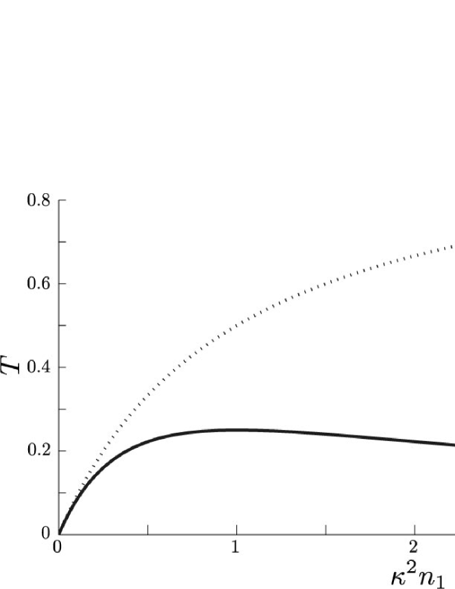
Figure 8: Scalings of the cross-Kerr ($T_{ab}$ - solid lines) and Kerr ($T_{cd}$ - dotted lines) nonlinearities as a function of $\kappa^{2}n_{1}=\Omega_{1}/\Omega_{2}$ for the case of a weak coherent pulse applied to the $|a\rangle-|b\rangle$ transition and the unknown (possibly single photon) field applied to the $|c\rangle-|d\rangle$ transition. The maximum of $T_{ab}$ occurs for the case that $\Omega_{1}=\Omega_{2}$.

The correct way to explore the nonlinear effect and hence QND measurement of the unknown field on the probe is to determine the Q-function of the state after the interaction. To effect a QND measurement, we require the Q-functions of the probe beam with and without a single photon in the channel being monitored to be distinguishable. Explicitly, returning to Eq. 46 we take the initial state of the probe field to be a coherent state $|\alpha\rangle$, with mean photon number $|\alpha|^{2}$. After interacting with this susceptibility, $K_{ab}$ for a period of time $t$, the probe will be in the state

$$|\alpha^{\prime}\rangle=\exp\left(-\frac{|\alpha|^{2}}{2}\right)\sum_{n_{1}=0}^{\infty}\frac{\alpha^{n_{1}}}{\sqrt{n_{1}!}}\exp\left(iK_{ab}t\right)|n_{1}\rangle,$$ (54)

and recall that $K_{ab}$ is a function of both $n_{1}$ and $n_{3}$. Note that in general $|\alpha^{\prime}\rangle$ will not be a coherent state following the interaction. We may define the Q-function for the state after interacting with the non-linear medium, which is

$$Q(\beta) = |\langle\beta|\alpha^{\prime}\rangle|^{2},$$ (56)

$$= \sum_{n_{1}=0}^{\infty}\frac{\exp\left(-\frac{|\alpha|^{2}+|\beta|^{2}-2n_{1}}{2}\right)}{\sqrt{2\pi n_{1}}}\left(\frac{\alpha\beta^{*}}{n_{1}}\right)^{n_{1}}\exp\left(iK_{ab}t\right)\times$$

$$\sum_{m_{1}=0}^{\infty}\frac{\exp\left(-\frac{|\alpha|^{2}+|\beta|^{2}-2m_{1}}{2}\right)}{\sqrt{2\pi m_{1}}}\left(\frac{\alpha^{*}\beta}{m_{1}}\right)^{m_{1}}\exp\left(-iK^{*}_{ab}t\right)$$

Note that as required, when $\Omega_{3}=0$ (i.e. the case of no-photon on the $|c\rangle-|d\rangle$ channel), $K_{ab}=0$ and the Q-function is simply the same Q-function expected for no interaction, i.e. there is no self-Kerr modulation.

The candidate system for realising a QND measurement that we are considering is a monolithic single-mode diamond waveguide (at $637~{}\mathrm{nm}$ containing NV^- centres, which is being pursued using a number of different fabrication strategies e.g. [60, 62, 76]. The energy levels show many possible configurations for achieving the four-state system under consideration [16, 66] and we will not delve further into these schemes, apart from noting that the transition dipole moments can be achieved and to some extent tuned in situ. Maximal coupling requires the smallest width single mode waveguides, which for the zero phonon line of NV^- corresponds to a cross section of around $200\times 200~{}\mathrm{nm}^{2}$. To avoid potential cross coupling between centres, we require an inter-centre spacing at least around $1~{}\mu\mathrm{m}$, which for the waveguide under consideration corresponds to an atomic density of $\mathcal{N}=4\times 10^{20}~{}\mathrm{m}^{-3}$. This level is dilute but achievable using ion implantation into ultra-low N synthetic diamond (e.g. Ref. [77]). Also for NV diamond, we have $\varepsilon_{R}\sim 10$ and $\mu_{ab}\sim 10^{-30}$ on the zero-phonon line transition.

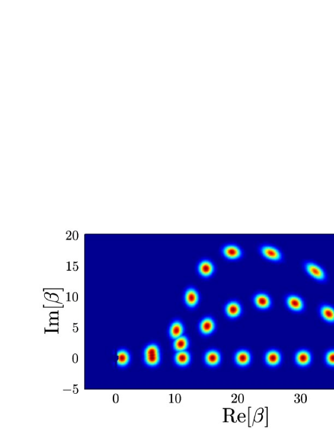
Figure 9: Q-functions for various conditions necessary for QND measurements using realistic parameters. The three sets of radial distributions correspond to the output probe beam when the signal has 0, 1 or 2 photons. Sets of distributions at constant radius from the origin are grouped with equal $|\alpha\rangle$. The increase in effective resolution with increasing $\alpha$ is demonstrated in this plot, and as discussed in the text, there is no apparent self-nonlinear processes. Parameters were chosen to correspond closely to expected EIT conditions in low N diamond containing NV^- colour centres, and these of reported in Table 1.

To determine the bandwidth of the pulse to be measured, we rearrange Eq. 20 for an absorption of $\mathcal{A}=1\%$. This implies that the bandwidth of probe and single photon field should be $f=8.9\times 10^{-3}\Gamma=740~{}\mathrm{kHz}$, or approximately $\Gamma/100$. With this bandwidth, we may immediately determine the single photon Rabi frequency, which from Eq. 43 is $\tilde{\Omega}_{3}=195\mathrm{MHz}$. The group velocity depends on the EIT condition and also the number of photons in the probe field.

Under these assumptions, and assuming the reduced inhomogeneous broadening for NVD on the zero phonon line that has been observed in low N diamond [16, 61, 78] of $\gamma=10~{}\mathrm{GHz}$, we are now able to fully model the rotation of the probe field in the QND measurement. Results from simulation are shown in Fig. 9 which shows the Q-function for various values of $\alpha$ and number of photons in the signal beam (field 3). A full list of parameters used in the calculations are provided in Table 1.

Fig. 9 shows families of Q-functions for the state of the probe field after traversing the EIT medium. There are three sets of lines. The lowest, horizontal set corresponds to the case that the signal field (field 3) had no photons, and represents the unperturbed probe field. This highlights the fact that the three-state EIT system does not exhibit self-phase modulation. Each point along this set corresponds to increasing $\alpha$ from 1 to 40. The upper two curves correspond to the probe field after traversing the medium with the signal field in the one photon (middle curve) or two photon (highest curve) state respectively, with $\alpha$ increasing to the right as before. QND measurement can be inferred whenever the Q-functions of the probe field corresponding to 0, 1 and 2 signal photons do not overlap. This can be seen clearly in the regime $\alpha>\sim 15$ (fourth set of Q-functions). Note that the phase shift is not linear in the regimes we are considering, and is greater than would be expected from the simple linear phase shift from an ideal cross-Kerr medium. This is likely due to the presence of higher-order nonlinearities in the regime $\Omega_{1}=\Omega_{2}$, although we have not made a detailed study of them. The distinguishability is maximised at around $\alpha\sim 25$ for these parameters. Note that this is earlier than the maximum expected from $T_{ab}$, which we attribute to group velocity dispersion reducing the effective interaction time for certain modes of the probe field. A complete study of these processes is beyond the scope of this work. A further point to note is that although QND discrimination can be made with very high certainty for $\alpha>\sim 14$, there is some noticeable distortion, especially in the 2-signal photon branch. This indicates that further work is required before strong claims of the effectiveness of this scheme for quantum gate operation can be made.

Table 1: Parameters for NV diamond waveguide system under consideration as QND gate

Waveguide dimensions	$w_{0}\times w_{0}\times l=200~{}\mathrm{nm}\times 200~{}\mathrm{nm}\times 200~{}\mu\mathrm{m}$
Atomic concentration	$\mathcal{N}=4\times 10^{20}~{}\mathrm{m}^{-3}$
Dipole moment (ZPL)	$\mu_{ab}=10^{-30}~{}\mathrm{Cm}^{-1}$
Transition frequency	$\lambda=637~{}\mathrm{nm}$
Relative permittivity of diamond	$\epsilon_{R}=10$
Homogeneous linewidth	$\Gamma=83~{}\mathrm{MHz}$
Inhomogeneous linewidth	$\gamma=10~{}\mathrm{GHz}$
Pulse bandwidth	$f=740~{}\mathrm{kHz}$
Semiclassical Rabi frequency	$\Omega_{2}=\Gamma/10$
Field ratios	$\kappa=\tilde{\Omega}_{1}/\Omega_{2}=1/50$
Signal per photon Rabi frequency	$\tilde{\Omega}_{3}=\frac{\lambda}{4\pi}\sqrt{3\Gamma f\mathcal{N}l}=195~{}\mathrm{MHz}$
Detuning scaling	$J=1/6$
Group velocity	$v_{g_{ab}}=\frac{c\varepsilon_{0}\varepsilon_{R}\hbar\Omega_{2}^{2}}{\omega\mathcal{N}\mu_{ab}^{2}}\left(\kappa^{2}n_{1}+1\right)=2.88\times 10^{4}\left(\frac{n_{1}}{2500}+1\right)~{}\mathrm{ms}^{-1}$

The parameters used in the equations used to generate the results shown in Fig. 9 are fairly typical of what has already been achieved or will be soon achieved in NVD. With variations in the parameters, there will be changes in the resulting phase shifts, but the parameters that we chose were not “fine tuned”.

5 Conclusions

We have performed investigations of three-state EIT in an inhomogeneously broadened sample with the aim of determining the necessary conditions for performing a quantum non-demolition measurement in a realistic solid-state medium, diamond containing the nitrogen-vacancy colour centre. Our results suggest that even in the presence of the relatively large inhomogeneous linewidth of these systems, QND measurements are possible using relatively modest extensions of the existing state of the art (demonstration of single mode waveguides of order $200~{}\mu\mathrm{m}$ long, and group velocity compensated propagation). These conclusions add substantial impetus to the ongoing push for diamond based quantum photonics and offer increased support for quantum computing based on weak nonlinear interactions.

References

References

- [1] Dowling JP and Milburn GJ 2003 Philosophical Transactions of the Royal Society of London Series A: Mathematical, Physical and Engineering Sciences 361, 1655
- [2] Harris SE, Field JE and Imamoğlu A 1990 Phys. Rev. Lett.64, 1107
- [3] Boller K-J, Imamoğlu A, and Harris SE 1991 Phys. Rev. Lett.66, 2593.
- [4] Scully MO and Fleischhauer M 1992 Phys. Rev. Lett.69, 1360
- [5] Merriam AJ, Sharpe SJ, Xia H, Manuszak D, Yin GY and Harris SE 1999 Opt. Lett. 24, 625
- [6] Dorman C, Kucukkara I and Marangos JP 2000 Phys. Rev. A, 61 013802
- [7] Harris SE and Yamamoto 1998 Phys. Rev. Lett.81, 3611
- [8] R. G. Beausoleil, W. J. Munro, D. A. Rodrigues, and T. P. Spiller 2004 J. Mod. Opt. 51, 2441.
- [9] Tucker RS, Ku PC and Chang-Hasnain CJ 2005 Journal of Lightwave Technology 23, 4046
- [10] Matsko AB, Strekalov D, Savchenkov AA and Maleki L 2007 Phys. Rev. A 76 013806
- [11] Zibrov AS, Lukin MD, Hollberg L, Nikonov DE, Scully MO, Robinson HG and Velichansky VL 1996 Phys. Rev. Lett.76, 3935
- [12] Ham BS, Hemmer PR and Shahriar MS 1997 Optics Communications 144, 227
- [13] Wei C and Manson NB 1999 J. Opt. B: Quantum Semiclass. Opt.1, 464
- [14] Hemmer PR, Turukhin A, Shahriar MS and Musser J 2001 Opt. Lett. 26, 361
- [15] Kuznetsova E, Kocharovskaya O, Hemmer P and Scully MO 2002 Phys. Rev. A 66, 063802
- [16] Santori C, Fattal D, Spillane SM, Fiorentino M, Beausoleil RG, Greentree AD, Olivero P, Draganski M, Rabeau JR, Reichart P, Gibson BC, Rubanov S, Huntington ST, Jamieson DN and Prawer S 2006 Optics Express 14, 7986
- [17] Santori C, Tamarat P, Neumann P, Wrachtrup J, Fattal D, Beausoleil R, Rabeau J, Olivero P, Greentree AD, Prawer S, Jelezko F and Hemmer P 2006 Phys. Rev. Lett.97, 247401
- [18] Mayer Alegre TP, Santori C, Medeiros-Ribeiro G and Beausoleil RG 2007 Phys. Rev. B 76, 165205
- [19] Chen HX, Durrant AV, Marangos JP and Vaccaro JA 1998 Phys. Rev. A 58, 1545
- [20] Hau LV, Harris SE, Dutton Z and Behroozi CH 1999, Nature (London) 397, 594
- [21] Imoto N, Haus HA and Yamamoto Y 1985 Phys. Rev. A 32, 2287
- [22] Munro WJ, Nemoto K, Beausoleil RG and Spiller TP 2005 Phys. Rev. A 71, 033819
- [23] Nemoto K and Munro WJ 2005 Phys. Lett. A 344, 104
- [24] Nemoto K and Munro WJ 2004, Phys. Rev. Lett.93, 250502
- [25] Munro WJ, Nemoto K and Spiller TP 2005 New J. Phys.7, 137
- [26] Munro WJ, Nemoto K, Spiller TP, Barrett SD, Kok P and Beausoleil RG 2005 J. Opt. B: Quantum Semiclass. Opt.S135
- [27] Spiller TP, Nemoto K, Braustein SL, Munro WJ, van Loock P and Milburn GJ 2006, New J. Phys.8, 30
- [28] van Loock P, Ladd TD, Sanaka K, Yamaguchi F, Nemoto K, Munro WJ and Yamamoto Y 2006, Phys. Rev. Lett.96, 240501
- [29] Louis SGR, Nemoto K, Munro WJ and Spiller TP 2007, New J. Phys.9 193
- [30] Krauss TF 2007, J. Phys. D: Appl. Phys.40, 2666
- [31] Altug H and Vučkovic J 2005, Appl. Phys. Lett. 86, 111102
- [32] Fleischhauer M, Imamoglu A and Marangos JP 2005 Rev. Mod. Phys.77, 633
- [33] Schmidt H and Imamoglu A 1996 Opt. Lett. 21, 1936
- [34] Kash MM, Sautenkov VA, Zibrov AS, Hollberg L, Welch GR, Lukin MD, Rostovtsev Y, Fry ES and Scully MO 1999 Phys. Rev. Lett.82 5229
- [35] Turukhin AV, Sudarshanam VS, Shahriar MS, Musser JA, Ham BS and Hemmer PR 2002 Phys. Rev. Lett.88 023602
- [36] Imamoğlu A, Schmidt H, Woods G and Deutsch M 1997 Phys. Rev. Lett.79, 1467
- [37] Rebić S, Tan SM, Parkins AS and Walls DF 1999 J. Opt. B: Quantum Semiclass. Opt.1, 1490
- [38] Werner MJ and Imamoğlu A 2000 Phys. Rev. A 61, R011801
- [39] Greentree AD, Vaccaro JA, de Echaniz SR, Durrant AV and Marangos JP 2000 J. Opt. B: Quantum Semiclass. Opt.2 252
- [40] Hartmann MJ, Brandão FGSL and Plenio MB, 2006 Nature Physics 2 849
- [41] Bermel P, Rodriguez A, Johnson SG, Joannopoulos JD and Soljačić M 2006 Phys. Rev. A 74 043818
- [42] Birnbaum KM, Boca A, Miller R, Boozer AD, Northup TE and Kimble HJ 2005 Nature (London) 436 87
- [43] Yan M, Rickey EG and Zhu Y 2001 Phys. Rev. A 64 013412
- [44] de Echaniz SR, Greentree AD, Durrant AV, Segal DM, Marangos JP and Vaccaro JA 2001 Phys. Rev. A 64 013812
- [45] Paspalakis E and Knight PL 2002 J. Mod. Opt 49 87
- [46] Zubairy MS, Matsko AB and Scully MO 2002 Phys. Rev. A 65 043804
- [47] Greentree AD, Richards D, Vaccaro JA, Durrant AV, de Echaniz SR, Segal DM and Marangos JP 2003 Phys. Rev. A 67 023818
- [48] Rebić S, Vitali D, Ottaviani C, Tombesi P, Artoni M, Cataliotti F and Corbalán R 2004 Phys. Rev. A 70 032317
- [49] Lukin MD and Imamoğlu A 2000 Phys. Rev. Lett.84 1419
- [50] Wang ZB, Marzlin KP and Sanders BC 2006 Phys. Rev. Lett.97 063901
- [51] Vlasov YA, Petit S, Klein G, Hönerlage B and Hirlimann Ch 1999 Phys. Rev. E 60 1030
- [52] Vlasov YA, O’Boyle M, Hamann HF and McNab SJ 2005 Nature 483 65
- [53] Beveratos A, Kühn S, Brouri R, Gacoin T, Poizat J-P and Grangier P 2002 Eur. Phys. J. D 18 191
- [54] Jelezko F, Gaebel T, Popa I, Gruber A and Wrachtrup J 2004 Phys. Rev. Lett.92 076401
- [55] Jelezko F, Gaebel T, Popa I, Domhan M, Gruber A and Wrachtrup J 2004 Phys. Rev. Lett.93 130501
- [56] Gaebel T, Domhan M, Popa I, Wittmann C, Neumann P, Jelezko F, Rabeau JR, Stavrias N, Greentree AD, Prawer S, Meijer J, Twamley J, Hemmer PR and Wrachtrup J, Nature Physics 2 408
- [57] Hanson R, Mendoza FM, Epstein RJ and Awschalom DD 2006 Phys. Rev. Lett.97 087601
- [58] Dutt MVG, Childress L, Jiang L, Togan E, Maze J, Jelezko F, Zibrov AS, Hemmer PR and Lukin MD 2007 Science 316 1312
- [59] Wang CF, Choi YS, Lee JC, Hu EL, Yang J and Butler JE 2007 Appl. Phys. Lett. 90, 081110
- [60] Olivero P, Rubanov S, Reichart P, Gibson B, Huntington S, Rabeau J, Greentree AD, Salzman J, Moore D, Jamieson DN and Prawer S 2005 Advanced Materials 17, 2427
- [61] Greentree AD, Olivero P, Draganski M, Trajkov E, Rabeau JR, Reichart P, Gibson BC, Rubanov S, Huntington ST, Jamieson DN and Prawer S, J. Phys.: Condens. Matter18, S825
- [62] Fairchild BA, Olivero P, Rubanov S, Greentree AD, Waldermann F, Taylor RA, Walmsley I, Smith JM, Huntington S, Gibson BC, Jamieson DN, and Prawer S 2008 Advanced Materials 20, 4793.
- [63] Rabeau JR, Huntington ST, Greentree AD and Prawer S, Appl. Phys. Lett. 86, 134104
- [64] Redman D, Brown S and Rand SC 1992 J. Opt. Soc. Am. B 9, 768
- [65] Tamarat Ph, Gaebel T, Rabeau JR, Khan M, Greentree AD, Wilson H, Hollenberg LCL, Prawer S, Hemmer P, Jelezko F and Wrachtrup J 2006 Phys. Rev. Lett.97, 083002
- [66] Tamarat Ph, Manson NB, Harrison JP, McMurtrie RL, Nizovtsev A, Santori C, Beausoleil RG, Neumann P, Gaebel T, Jelezko F, Hemmer P and Wrachtrup J 2008 New J. Phys.10, 045004
- [67] B. W. Shore, The Theory of Coherent Atomic Excitation, Volume 2, Multilevel Atoms and Incoherence (John Wiley and Sons, New York, 1990).
- [68] Wielandy S and Gaeta AL 1998 Phys. Rev. A 58, 2500.
- [69] Müller M, Homann F, Rinkleff R-H, Wicht A, and Danzmann K 2000 Phys. Rev. A 62, 060501(R).
- [70] Gea-Banaloche J, Li Y, Jin S, and Xiao M 1995 Phys. Rev. A 51, 576.
- [71] Vemuri G and Agarwal GS 1996 Phys. Rev. A 53, 1060.
- [72] Allen L and Eberly J H 1975 Optical Resonance and Two Level Systems (Chichester: Wiley)
- [73] Rohde PP, Munro WJ, Ralph TC, van Loock P and Nemoto K 2008 Quantum Information and Computation 8, 0053.
- [74] Kok P 2008 Phys. Rev. A 77, 013808.
- [75] Beausoleil RG, Munro WJ, Spiller TP 2004 J. Mod. Opt. 51 1559.
- [76] Hiscocks MP, Kaalund CJ, Ladouceur F, Huntington ST, Gibson BC, Trpkovski S, Simpson D, Ampem-Lassen E, Prawer S, Butler JE 2008 Diamond and Related Materials 17, 1831.
- [77] Meijer J, Burchard B, Domhan M, Wittmann C, Gaebel T, Popa I, Jelezko F and Wrachtrup J 2005 Appl. Phys. Lett. 87, 261909
- [78] Waldermann FC, Olivero P, Nunn J, Surmacz K, Wang ZY, Jaksch D, Taylor RA, Walmsley IA, Draganski M, Reichart P, Greentree AD, Jamieson DN, Prawer S 2007 Diamond and Related Materials 16, 1887