Totally Asymmetric Exclusion Process with Hierarchical Long-Range Connections

Abstract

A non-equilibrium particle transport model, the totally asymmetric exclusion process, is studied on a one-dimensional lattice with a hierarchy of fixed long-range connections. This model breaks the particle-hole symmetry observed on an ordinary one-dimensional lattice and results in a surprisingly simple phase diagram, without a maximum-current phase. Numerical simulations of the model with open boundary conditions reveal a number of dynamic features and suggest possible applications.

I Introduction

Physicists have long hoped to understand non-equilibrium phenomena as well as they understand equilibrium phenomena (Schmittmann95, ). Certain non-equilibrium systems exist which reach a steady state, yet they do not obey detailed balance required for any equilibrium. The steady states are defined by the dynamics rather than an energy function. Exclusion processes are widely studied as models of particle transport and were first introduced for the kinetics of bio-polymerization on nucleic acid templates (citeulike:1532138, ). They have since been related to other phenomena such as surface growth (Barabasi95, ), traffic flow (Biham92, ; Nagel92, ; Nagel95, ), and the statistics of DNA sequence alignment (citeulike:3175269, ). The totally asymmetric exclusion process (TASEP) represents a rare example of an exactly solvable model with a non-equilibrium steady state that allows a deep, analytic insight into the phenomenology of critical behavior beyond thermodynamic equilibrium (citeulike:1341557, ; citeulike:3196043, ; citeulike:3196051, ). TASEP and related models exhibit non-equilibrium phase transitions which have no analog in equilibrium systems, such as a phase transition in one dimension.

TASEP describes particles conducting nearest neighbor jumps along one direction within a line of sites. There is no passing, and jumps of particles to an occupied forward site are excluded, leading to jamming. The model has been solved first in a mean-field treatment (citeulike:1341557, ) and subsequently in full detail (citeulike:3196043, ; citeulike:3196051, ), and has since inspired a large number of variations (Hinrichsen00, ; Mobilia08, ). Yet, the phase diagram has proven quite robust under those changes. Even admitting long-range jumps, which allows particles to pass forward by a stochastic long-range jump according to a Levy distribution if the target site is unoccupied, leaves the phase diagram surprisingly unchanged (citeulike:3163805, ).

The purpose of this paper is to introduce jumps into the TASEP in a non-stochastic way by using a network with predetermined long-distance jumps and to study it’s effect on the phases and transitions. Such a quenched structure is provided by the recently introduced network HN3. HN3 has a hierarchical structure, combining a simple one-dimensional backbone with a sequence of long-range links. Interesting properties for other statistical models on HN3 have already been described in Ref. (SWPRL, ). The process on HN3 (HN3-TASEP) might prove to be a benign enough extension beyond that in one dimension ($1d$-TASEP) such that analytical insights remain possible, even though introducing quenched long-range connections removes the particle-hole symmetry. Here, we show numerically that HN3 alters the phase diagram significantly. In fact, only two phases remain, separated by a sharp first-order transition. Our results suggest that there might indeed be a simple solution for this model which would take the analytic treatment of exclusion processes beyond one dimension. The observed behavior suggests that the hierarchical lattice used here also provides an efficient switch for a simple, one parameter storage-and-release system.

There are some real systems to which an exclusion process with particles passing each other applies. For instance, as pointed out in Ref. (citeulike:3175269, ), some proteins regulate genes by binding to DNA and search for a specific target site by continuous dissociation and re-association with the DNA. In the dissociation process, they may fully dissociate or stay within the range of electrostatic forces of the DNA. In another application, HN3-TASEP could model traffic (Biham92, ; Nagel92, ; Nagel95, ) with expressways, which also function as quenched shortcuts. The hierarchical but geometric structure of HN3 may even apply to a multi-level transport system such as a package delivery service with many door-to-door vans, a number of intercity trucks and trains, and a few transcontinental flight routes.

Our discussion proceeds with a review of the ordinary $1d$-TASEP in the next section, followed in Sec. III by a description of the hierarchical lattice geometry employed here. In Secs. IV and  V, we present our numerical results and analytic approach, respectively. In Sec. VI we discuss the implications of our findings and provide our conclusions in Sec. VII.

II TASEP on a line

The totally asymmetric exclusion process in one dimensional ($1d$-TASEP), where particles always move in one direction, is a model which has several phases with first and second-order transitions (citeulike:1341557, ; citeulike:3196043, ; citeulike:3196051, ). It is defined on a one-dimensional lattice of length $L$. Each site of the lattice, labeled by $i$, is either occupied or unoccupied by a particle, and accordingly has an occupation number $\tau_{i}$ which is either 1 or 0. Particles on the lattice may only move in one direction, which we will say is to the right, and they may hop one site to the right only if that site is unoccupied. Typically, the system is updated random sequentially, that is, particles are selected to move one at a time in random order. The average density $\rho$ is defined as $N/L$, where $N$ is the number of particles in the system. The average current $J$ is defined as the average number of particles that move through a point on the lattice per time step. For periodic boundary conditions, $N$ is fixed, while for open boundary conditions, as considered here, $N$ is allowed to fluctuate, which induces several phases characterized by different properties for $\rho$ and $J$. The two open boundaries are connected to a large reservoir of particles, so that the rate of particles hopping onto the lattice at the first site is $\alpha,$ and the rate of particles removed from the last site is $\beta$, providing two independent parameters. Both define a parameter space for which the different phases appear, see Fig. 1. Their rates are between 0 and 1, as no more than one particle may appear or disappear on the boundary in a single trial.

Fig. 1 shows three phases distinguished by their average densities and currents in the steady state, first found in Ref. (citeulike:1341557, ). The low density (LD) phase has $\rho_{LD}=\alpha$ and $J_{LD}=\alpha(1-\alpha)$, the high density (HD) phase has $\rho_{HD}=1-\beta$ and $J_{HD}=\beta(1-\beta)$, and the maximum current (MC) phase has $\rho_{MC}=1/2$ and $J_{MC}=1/4$. The HD and LD phases are related because of particle-hole symmetry. The transitions between the LD and HD phases and the MC phase are continuous. The line between the LD and HD phases is called the “shock phase” (SP). This transition is not continuous and the system reaches a state of coexistence between the two phases. On the lattice there is a region with low density and a region of high density separated by microscopically small “shock”, which diffuses between the ends of the lattice.

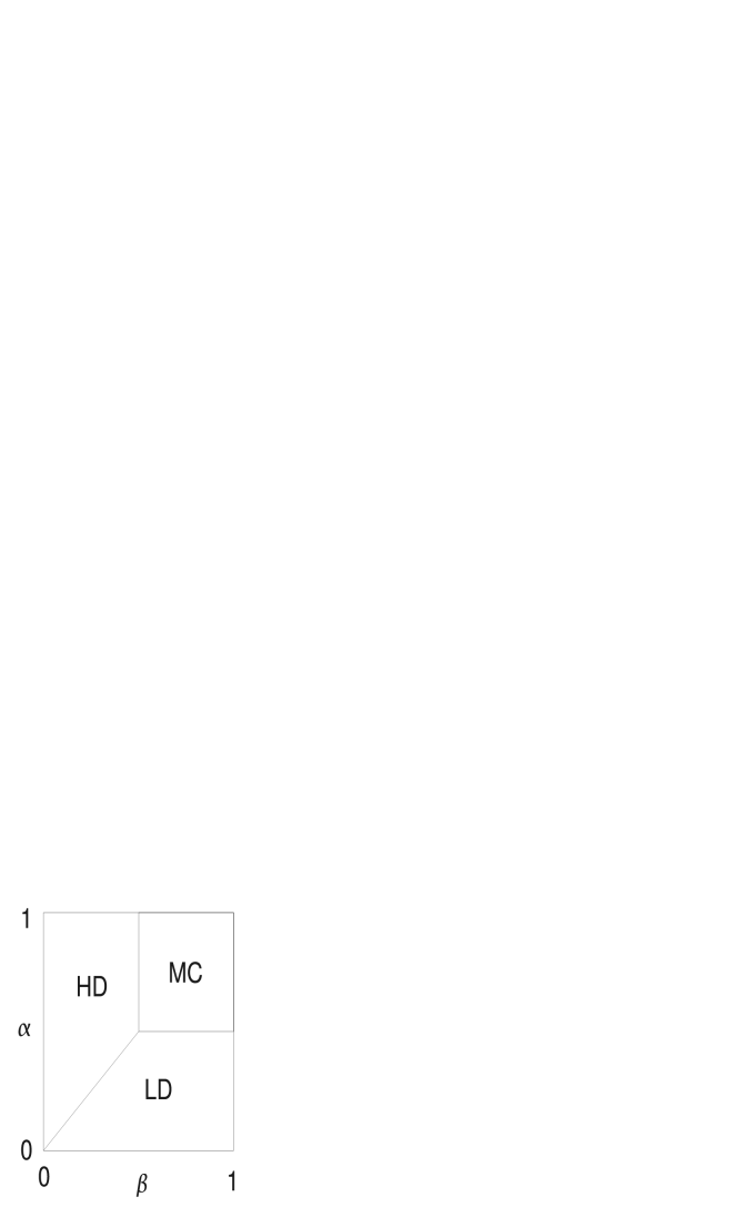
Figure 1: Phase diagram of the $1d$-TASEP with high density (HD), low density (LD) and maximum current (MC) phases. The injection rate is $\alpha$ and the removal rate is $\beta$.

$1d$-TASEP has been solved exactly with recursive equations (citeulike:1341557, ; citeulike:3196051, ), as well as a more advanced matrix formulation (citeulike:3196043, ). The process is completely described by the change in occupations on affected sites for an update at a bulk-site $i$ during the time interval $\left[t,t+dt\right]$. Such an update merely alters site $i$ and $i+1$:

$$\tau_{i}(t+dt) = \tau_{i}(t)\tau_{i+1}(t)$$ (1)

$$\tau_{i+1}(t+dt) = \tau_{i+1}(t)+\left[1-\tau_{i+1}(t)\right]\tau_{i}(t),$$

all other sites remain unchanged. Special treatment obtains for each of the two boundary sites. When the update selects to inject a new particle into the system, that particle attempts to occupy site $i=1$ with probability $\alpha$, if that site is open. When the last site, $i=L$, is selected for an update, it unloads an occupying particle with probability $\beta$.

These master equations, as well as those boundary conditions, can be averaged over noise, eliminating all fluctuations, and written as single differential equation describing the time evolution of the system. Assuming the existence of a steady state, $\partial_{t}\left\langle\tau_{i}\right\rangle=0$, leads to a system of algebraic equations at most quadratic in $\left\langle\tau_{i}\right\rangle$, which can be solved recursively.

Many variations of TASEP have been studied, such as those with parallel updates, multiple species of particles, and extended particle sizes (Mobilia08, ). Remarkably, the phase diagram is essentially the same for many variations. For example, one variation studied recently introduced long range jumps so that particles may jump past each other (if the target site is unoccupied) to study the changes to the phases and transitions (citeulike:3163805, ). These jumps are stochastic Levy flights, i. e. a distance $l$ is reached with probability $p_{l}\sim l^{-(1+\sigma)}$ depending on a parameter $\sigma>0$. Even with long jumps and reordering (“passing”) of particles, the diagram has the same three phases as in Fig. 1.

III TASEP on the Hierarchical Network HN3

HN3 is a network with a fractional dimension, which was introduced with the intention of studying small-world phenomena analytically (SWPRL, ). Small-world phenomena are found in many natural and man-made systems, such as neural networks and the internet (citeulike:99, ). The networks are characterized by having a mixed structure (Boccaletti06, ), with connections between geometrically nearby neighbors as well as long distance connections, which drastically reduce the typical path length between any two nodes. The HN3 network does not have the same mean-field properties usually associated with such networks. For instance, average path lengths scale with $\sqrt{L}$ instead of $\ln(L)$ with system size $L$. But HN3 is constructed in a hierarchical manner that is conducive for the renormalization group, which is a technique that takes advantage of the self-similarity of systems (SWN, ).

HN3 consists of a one dimensional line as a backbone with $L=2^{k}+1$ sites, where $k$ is a positive integer which defines the number of hierarchies. To make the long distance connections, we consider an integer $i\leq k$, which defines the level of the hierarchy, and $j$, an integer which parameterizes the connection in a hierarchy. All sites (except for $n=0$) are then uniquely represented by

$$n=2^{i}(2j+1).$$ (2)

For example, for $i=0$, $n$ runs over all the odd integers, and $i=1$ makes $n$ to be all integers once divisible by 2 (i.e. 2, 6, 10, …), etc. Connections are made between neighbors within the hierarchy, so for $i=0$, site 1 connects to 3, 5 to 7, etc, and for $i=1$, 2 to 6, 10 to 14, etc. It is possible to make a more complex network, HN4, by connecting two neighbors in the hierarchy to every site. Fig. 2 shows the HN3 network for $k=5$. The first, middle, and last site are special in that they have no long range connections (the first and last site, 0 and $L$, are not shown). All the other sites are connected to three other sites. The distance between the ends of the HN3 network are known to be proportional to $\sqrt{L}$, which is similar to the diagonal on a square lattice with $L$ sites.

Figure 2: The HN3 network consists of a one-dimensional backbone and a hierarchy of long distance connections.

In an implementation of TASEP on the HN3 network (which we shall refer to as HN3-TASEP), on sites with a long-range forward link, particles have the possibility to move to two different sites. To obtain an interesting dynamics we decided to have the chosen particle attempt a jump to the long distance site first, and if that site is occupied, to reach the short distance site as in $1d$-TASEP. For such a site, representing half of all sites, jamming is somewhat alleviated, as it can free itself with a higher probability. In turn, the other half of all sites, possessing one extra incoming link instead, occupation and jamming is far more likely.

We will also study a family of models that interpolates between $1d$-TASEP and HN3-TASEP, using a probabilistic update rule: At each update, with a probability $r$, a long-range jump is attempted first but if such a jump does not succeed, a nearest-neighbor forward-jump is attempted. For $r=0$, no long-range jump ever occurs, representing the $1d$-TASEP case, while $r=1$ corresponds to the HN3-TASEP case. We find that the nature of TASEP changes discontinuously for $r>0$, numerically signaled by the disappearance of the MC phase (and the associated $2nd$-order transitions), while the shock persists at any $r$. We suspect that such discontinuity can be attributed to the broken particle-hole symmetry, which only holds for strictly $r=0$.

IV Numerical Results

We implemented a Monte Carlo simulation for HN3-TASEP as follows. First a particle is randomly chosen from $N$ particles on the lattice plus one virtual particle. If a lattice particle is selected, it is moved forward one site if that site is unoccupied. If a virtual particle is selected, a random number between zero and one is generated, and if it is less than $\alpha$, a particle is placed at the first site of the lattice unless it is occupied. If a particle is selected which is at the end of the lattice, a random number is generated, and if it is less than $\beta$, that particle is removed. A sequence of $N+1$ attempts to move particles constitute one Monte Carlo Sweep (MCS). The number of lattice sites for every result in this report was set at $L=1023$, unless otherwise stated. The simulations were run for $10^{6}$ MCS, and the first $10^{5}$ MCS were discarded to allow the system reached a steady state. Current and density for the system were recorded every 100 MCS and averaged over to characterize the steady state.

Figure 3: to compare with that of $1d$-TASEP in Fig. 1 The density $\rho$ (top) and current $J$ (bottom) of TASEP on HN3 on a grid of 25 values each for $\alpha$ and $\beta$.

The behavior of HN3-TASEP is quite different from $1d$-TASEP (citeulike:1341557, ), which can be seen when $\rho$ and $J$ are plotted for a grid of 25 by 25 values of $\alpha$ and $\beta$ in Fig. 3. The HD and LD phases are present, but the MC phase is conspicuously missing. The magnitude of $\rho$ and $J$ are significantly altered. (Note that the current is measured here at the exit site, which every particle moving through the system must pass; the same is not true for most other sites!) The density is much higher in the HD phase and much lower in the LD phase when the HN3 shortcuts are present. In fact, throughout each phase, the density remains almost constant. The lattice is able to fill itself with particles more efficiently in HD and remove them more efficiently in LD when there are more connections between sites. Based on the density plot in Fig. 3, in Fig. 4 we extract the outlines of a phase diagram for HN3-TASEP to compare with that of $1d$-TASEP in Fig. 1.

Figure 4: Phase diagram of HN3-TASEP with only a high density (HD) and low density (LD) phases, to compare with that of $1d$-TASEP in Fig. 1. The data points are extracted from Fig. 3, the dashed line represents a simple polynomial fit, and the dotted line is crude approximation to the phase line resulting from the linearized mean-field equations in Sec. V.

Considering that HN3 is a hierarchical network, it is worth noting that the results are smooth and not heterogeneous in any complicated fashion (unlike the average occupation on sites, see below). Similar to $1d$-TASEP, in the HD phase the current does not appear to vary with $\alpha$, and in the LD phase it does not change appreciably with $\beta$. To make sure the transition is first-order, $\rho$ is plotted for values of $\alpha=1$ and $\beta$ between 0.7 and 0.8 for two lattice sizes in Figs. 5. The transition is less pronounced on a smaller lattice, which indicates the transition is most likely sharp in the thermodynamic limit: The data indicates that in the thermodynamic limit $L\to\infty$ the lattice is completely filled almost everywhere in the high-density phase, and it is completely empty in the low-density phase. This result enables a simplifying Ansatz to the equations in Sec. V below.

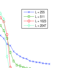
Figure 5: Top: Density during the transition from HD to LD for lattices of size $L=255,$ 511, 1023, and 2047 at $\alpha=1$. The total number of Monte Carlo Sweeps (MCS) for each data point was $5\,10^{6}$. Bottom: The density for the different values of $\beta$ plotted against $1/L$. The values range over $\beta=0.7\ldots 0.8$ in steps of 0.08. The dashed line in the middle corresponds to $\beta=0.748$, which appears closest to the transition, exhibits a significant error as the stationary “shock” state is hard to sample. But almost all data below extrapolates to a value of $\rho$ consistent with full packing, while all data for values of $\beta$ above the transition extrapolates to an empty lattice, $\rho\approx 0$.

If one considers a single particle moving through an empty $1d$ lattice, it moves one site every step and $v=1$. Since in HN3 the shortest end-to-end path is of length $\sim\sqrt{L}$ (SWPRL, ), the time for a particle to traverse it is $\sim\sqrt{L}$ and, hence, $v=L/T\approx\sqrt{L}$. The velocity is dependent on the lattice size, and is unbounded for large lattices, although this definition of velocity is based on the notion that the length of a lattice is equal to it’s number of sites. In the LD phase the particles can follow the shortcuts, since they are usually unoccupied. In the HD phase most sites, including ones at the end of shortcuts, are occupied, so the particles have few opportunities to take a shortcut and they travel along the backbone, which limits the velocity to $v<1$. Fig. 6 shows the velocity for a parameter range across the transition. In the HD phase the velocity is indeed $<1$, but in the LD phase it is $\gg 1$. The velocity can also be examined for the case $\beta=1$, where the system is always in the LD phase, as shown in Fig. 7. For small $\alpha$, the number of particles is very low and they can take all of the shortcuts. The velocity is on the order of $16\approx\sqrt{L}/2$. As $\alpha$ increases, some of the shortcuts are occupied and the particles take trajectories that are a mix between shortcut and backbone movements, which decreases the average velocity. The $\sqrt{L}$-dependence of the transit time can be demonstrated through finite size scaling. Fig. 8 shows the average transit time at a low injection rate and high removal rate for many lattice sizes, and it approximately follows $\sqrt{L}$. The stair-casing effect between even and odd values of the hierarchy index $k$ is due to the fact that HN3 is strictly self-similar only for every second recursion of the hierarchy. In particular, as particles move left to right, they take every shortcut available, and on networks with odd $k$ they miss the opportunity to take the largest shortcut, which is part of the shortest path available.

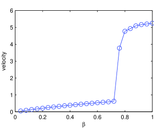
Figure 6: Average velocity of particles for $\alpha=1$ and varying $\beta$. The velocity is $v<1$ in the HD phase ($\beta\lesssim 0.75$), and $v\gg 1$ in the LD phase.

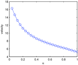
Figure 7: Average velocity of TASEP on HN3 for $\beta=1$.

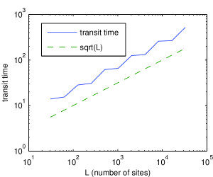
Figure 8: Average transit time versus lattice size L for $\alpha=0.01$ and $\beta=1$. The transit time shows a $\sqrt{L}$ dependence, which means particles are taking the shortest path on HN3. The stair-casing is due to particles on networks with odd $k$ only taking the second shortest path.

One may also keep track of the number of time steps it takes for each particle to cross the lattice. Fig. 9 shows a histogram of the transit times for $\beta=$1 and a small value of $\alpha$, so the particles are removed at the maximum rate and injected at a slow rate. There is a bimodal distribution which suggests particles are only taking a few distinct paths through the network, such as the shortest and second shortest paths. It is interesting that the bimodal distribution does not show up for other parts of the parameter space. When $\alpha$ is smaller, the particles follow only the shortest path, and there is only one peak. The width of the peak originates with the update procedure, as not every particle is updated at every Monte Carlo sweep, thus leading to fluctuations in transit times. When $\alpha$ becomes larger there is some blockage of shortcuts and the particles immediately follow many different paths. There is only one peak in the distribution of transit times with a long tail and there is no clear separation between fast moving particles and slow moving particles. The number of particles taking the shortest path is probably very small for any set of parameters except when the density is very low.

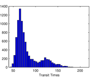
Figure 9: Distribution of the transit times at $\alpha=0.1$, and $\beta=1$.

We note that the shock phase looks very different on HN3 from that in $1d$-TASEP. Fig. 10 shows a typical time evolution of the occupation on the lattice at a point in the parameter space where $\rho$ was roughly 0.5 and can be compared to the shock phase in $1d$-TASEP (Hinrichsen00, ). It is clear that there is coexistence of the LD and HD phases, but there appears to be a hierarchy of boundary sites, depending on the range of the long connections of the originating site, as we might expect that there is more movement near sites with the longer connection.

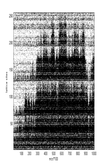
Figure 10: Time evolution of the shock phase in TASEP on HN3 on a lattice of size $L=255$. Each white pixel is an occupied site. Time is represented by 100 Monte Carlo sweeps.

A similar picture about the intricate internal dynamics within the lattice emerges from the average steady-state occupation $\left\langle\tau_{i}\right\rangle$ for each site, shown in Fig. 11. Smoothed over many sites, one could argue that the general trend is similar to that in $1d$-TASEP, where in LD the bulk density is constant, cumulating in a defined boundary layer near the exit, while in HD there is such a layer at the entrance, followed by a constant density plateau in the bulk (citeulike:1341557, ). Although in HN3-TASEP corresponding boundary layers are visible, the site-to-site density is extremely rough, owing to the heterogeneous mix of incoming and outgoing long-range jumps that belong to very different levels of the hierarchy and thus have very different efficiencies in transmitting particles. Our linear approximation to the steady-state equations in Sec. V manages to reproduce these heterogeneities very well.

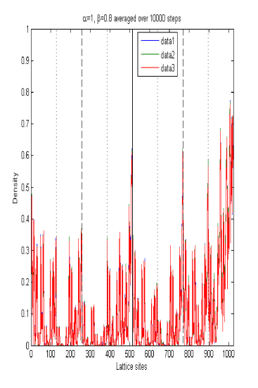
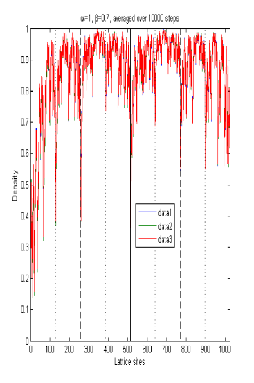
Figure 11: Average occupation $\left\langle\tau_{i}\right\rangle$ in the steady state on sites along the lattice backbone in HN3-TASEP in LD (top) and HD (bottom). In low density (LD), sites with the longer-range connections show more occupation as way-stations of short paths through the lattice that bypass particles away from sites belonging to lower levels of the hierarchy. In turn, in high density (HD) low-level sites get jammed up while sites with longer-range connections (especially forward) have an easier time to empty themselves. Note the boundary layers of increased jamming near the exit in LD and that of depletion at the entrance in HD.

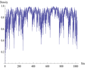
Figure 12: Average steady-state occupation $\left\langle\tau_{i}\right\rangle\approx 1-\epsilon_{i}$ on HN3-TASEP, as obtained analytically in the linearized approximation ($\epsilon_{i}\ll 1$) in Eq. (15) for HD. Aside from an arbitrary overall scale for the $\epsilon_{i}$, the pattern corresponds in great detail to that in Fig. 11, except for the boundaries.

V Analytic Treatment

To obtain a set of master equations such as those in Eq. (1) for HN3-TASEP, we have to distinguish two different kinds of sites. An IN-site $i$ simply has a long-range connection to a site $i-l$, preceding it by a distance $l$ in the lattice, in addition to its immediate predecessor and successor sites $i-1$ and $i+1$. Generically, at any level in the hierarchy, updates at an IN-site $i$ do not affect either of the predecessor sites, hence, the equations are similar to those in Eqs. (1):

$$\tau_{i}(t+dt) = \tau_{i}(t)\tau_{i+1}(t),$$ (3)

$$\tau_{i+1}(t+dt) = \tau_{i+1}(t)+\left[1-\tau_{i+1}(t)\right]\tau_{i}(t).$$

In turn, when the update occurs at an OUT-site $i$ with a long-range link to a successor site $i+l$, that site $i$, the immediate successor site $i+1$, and the long-range successor site $i+l$ are affected in a novel way in HN3-TASEP. In our choice of moving particles preferentially along the long links leads to a three-stage update process: Only if the long jump is blocked, a short jump to the successor site is attempted; if that is blocked as well, the particles remains on its site. These choices are expressed through the following equations for the updated site, its successor, and its long-range forward neighbor:

$$\tau_{i}(t+dt) = \tau_{i}(t)\tau_{i+1}(t)\tau_{i+l}(t),$$ (4)

$$\tau_{i+1}(t+dt) = \tau_{i+1}(t)+\tau_{i}(t)\left[1-\tau_{i+1}(t)\right]\tau_{i+l}(t),$$

$$\tau_{i+l}(t+dt) = \tau_{i+l}(t)+\tau_{i}(t)\left[1-\tau_{i+l}(t)\right].$$

Note that these equations are inherently cubic in the dynamic variables. Another complication is the lack of translational invariance, as these equations depend on a forward-distance $l$, which itself depends strongly on the hierarchical level that site $i$ belongs to. At least, the boundary conditions, affecting sites $i=0$ and $i=L$, are identical to $1d$-TASEP.

To make any progress at all, we already at this point consider the mean-field limit. The mean-field limit averages the dynamic variables over the noise, eliminating fluctuations and correlations, i. e. we set $\left\langle\tau_{i}\tau_{j}\right\rangle\sim\left\langle\tau_{i}\right\rangle\left\langle\tau_{j}\right\rangle=\tau_{i}\tau_{j}$, and allows us to arrive at a set of rate equations for the continuous variables $\tau_{i}$. We have to take full account of the lack of translational invariance along the line in HN3 by addressing the hierarchical level any site belongs to. All sites on the lowest level are of odd index $2j+1$, and they are alternately IN and OUT-sites. Say, all sites $4j+1$ are OUT-sites. While it is then clear that it has two successors, one and two steps ahead, and a single predecessor site, the latter itself may be an IN or an OUT-site. But depending on that, its update will affect our $4j+1$ site differently, and we make the further simplifying assumption of an equal balance between both possibilities. Hence, on average, site $4j+1$ is changed as

$$\tau_{4j+1}(t+dt) = \left(1-dt\right)\tau_{4j+1}(t)$$

$$+dt\,\tau_{4j+1}(t)\tau_{4j+2}(t)\tau_{4j+3}(t)$$

$$+\frac{dt}{2}\,\tau_{4j}(t)\left[1-\tau_{4j+1}(t)\right]$$

$$+\frac{dt}{2}\,\tau_{4j}(t)\tau_{4j+l}(t)\left[1-\tau_{4j+1}(t)\right],$$

where the distance $l$ furthermore depends on that predecessor site at $4j$. In order, the terms in Eq. (V) refer to either nothing changing with probability $1-dt$, our reference site $4j+1$ being updated itself [see the first of Eqs. (4)] with probability $dt$, or the predecessor site $4j$ being update with probability $dt/2$ for each of the two scenarios given. Similar considerations holds for the IN-sites at $4j+3$, with yet another complication arising from the incoming long-range predecessor site $4j+1$, whose potential update adds another term:

$$\tau_{4j+3}(t+dt) = \left(1-dt\right)\tau_{4j+3}(t)$$

$$+dt\,\tau_{4j+3}(t)\tau_{4j+4}(t)$$

$$+\frac{dt}{2}\,\tau_{4j+2}(t)\left[1-\tau_{4j+3}(t)\right]$$

$$+\frac{dt}{2}\,\tau_{4j+2}(t)\tau_{4j+2+l}(t)\left[1-\tau_{4j+3}(t)\right]$$

$$+dt\,\tau_{4j+1}(t)\left[1-\tau_{4j+3}(t)\right].$$

At all other levels in the hierarchy, matters somewhat simplify, as any even site clearly has an odd-indexed site preceding and following it, making the effect of long-range bonds fully apparent. In particular, sites $2(2j+1)$ at the next-to-bottom level all have an odd OUT-site $4j+1$ preceding it and the corresponding IN-site $4j+3$ following it, independent of whether they themselves are OUT or IN-sites. Still, in their own update behavior, OUT-sites at $2(4j+1)$ and IN-sites at $2(4j+3)$ at this level differ, and we get

$$\tau_{2\left(4j+1\right)}(t+dt)=\left(1-dt\right)\tau_{2\left(4j+1\right)}(t)$$ (7)

$$\quad+dt\,\tau_{2\left(4j+1\right)}(t)\tau_{2\left(4j+1\right)+1}(t)\tau_{2\left(4j+3\right)}(t)$$

$$\quad+dt\,\tau_{2\left(4j+1\right)-1}(t)\tau_{2\left(4j+l\right)+1}(t)\left[1-\tau_{2\left(4j+1\right)}(t)\right],$$

and

$$\tau_{2\left(4j+3\right)}(t+dt)=\left(1-dt\right)\tau_{2\left(4j+3\right)}(t)$$ (8)

$$\quad+dt\,\tau_{2\left(4j+3\right)}(t)\tau_{2\left(4j+3\right)+1}(t)$$

$$\quad+dt\,\tau_{2\left(4j+3\right)-1}(t)\tau_{2\left(4j+3\right)+1}(t)\left[1-\tau_{2\left(4j+3\right)}(t)\right]$$

$$\quad+dt\,\tau_{2\left(4j+1\right)}(t)\left[1-\tau_{2\left(4j+3\right)}(t)\right].$$

Finally, at any higher level $i\geq 2$ of the hierarchy, all sites $2^{i}\left(2j+1\right)$ only have odd-indexed IN-sites as predecessor and odd-indexed OUT-sites as successor. We get for OUT and IN-sites, respectively:

$$\tau_{2^{i}\left(4j+1\right)}(t+dt)=\left(1-dt\right)\tau_{2^{i}\left(4j+1\right)}(t)$$ (9)

$$\qquad+dt\,\tau_{2^{i}\left(4j+1\right)}(t)\tau_{2^{i}\left(4j+1\right)+1}(t)\tau_{2^{i}\left(4j+3\right)}(t)$$

$$\qquad+dt\,\tau_{2^{i}\left(4j+1\right)-1}(t)\left[1-\tau_{2^{i}\left(4j+1\right)}(t)\right],$$

and

$$\tau_{2^{i}\left(4j+3\right)}(t+dt)=\left(1-dt\right)\tau_{2^{i}\left(4j+3\right)}(t)$$ (10)

$$\qquad+dt\,\tau_{2^{i}\left(4j+3\right)}(t)\tau_{2^{i}\left(4j+3\right)+1}(t)$$

$$\qquad+dt\,\tau_{2^{i}\left(4j+3\right)-1}(t)\left[1-\tau_{2^{i}\left(4j+3\right)}(t)\right]$$

$$\qquad+dt\,\tau_{2^{i}\left(4j+1\right)}(t)\left[1-\tau_{2^{i}\left(4j+3\right)}(t)\right].$$

In the steady state, we consider $t\sim t+dt\to\infty$. Then, the above equations somewhat simplify, and we get from Eqs. (V-V):

$$\tau_{n} = \tau_{n}\tau_{n+1}\tau_{n+2}+\frac{1}{2}\tau_{n-1}\left(1-\tau_{n}\right)\left(1+\tau_{n-1+l}\right),\quad$$ (11)

$$\tau_{m} = \tau_{m}\tau_{m+1}+\frac{1}{2}\tau_{m-1}\left(1-\tau_{m}\right)\left(1+\tau_{m-1+l}\right)$$

$$\qquad+\tau_{m-2}\left(1-\tau_{m}\right),$$

at the lowest level, where we have set $n=4j+1$ for OUT-sites and $m=4j+3$ for IN-sites. Similarly, from Eqs. (7-8), we get

$$\tau_{n} = \tau_{n}\tau_{n+1}\tau_{n+4}+\tau_{n-1}\left(1-\tau_{n}\right)\tau_{n+1},$$ (12)

$$\tau_{m} = \tau_{m}\tau_{m+1}+\tau_{m-1}\left(1-\tau_{m}\right)\tau_{m+1}$$

$$\qquad+\tau_{m-4}\left(1-\tau_{m}\right),$$

here setting $n=2(4j+1)$ for the OUT-sites and $m=2(4j+3)$ for the IN-sites. Finally, the general case in the hierarchy from Eqs. (9-10) reduces to

$$\tau_{n} = \tau_{n}\tau_{n+1}\tau_{n+2^{i+1}}+\tau_{n-1}\left(1-\tau_{n}\right),$$ (13)

$$\tau_{m} = \tau_{m}\tau_{m+1}+\tau_{m-1}\left(1-\tau_{m}\right)$$

$$\qquad+\tau_{m-2^{i+1}}\left(1-\tau_{m}\right),$$

with $n=2^{i}(4j+1)$ for the OUT-sites and $m=2^{i}(4j+3)$ for the IN-sites for $i\geq 2$. Since the first and last bond in the lattice do not get bridged by a long-range jump, see Fig. 2, the boundary conditions are similar to those for $1d$-TASEP (citeulike:1341557, ):

$$\tau_{0}\left(1-\tau_{1}\right) = \alpha\left(1-\tau_{0}\right),$$ (14)

$$\beta\tau_{L} = \tau_{L-1}\left(1-\tau_{L}\right),$$

with $L=2^{k}$.

Although the steady state has simplified the equations somewhat, their main difficulties remain their lack of symmetry and their cubic order. Yet, our numerical results in Sec. IV, particularly Fig. 3, suggest a very simple phase structure with $\tau_{i}\sim 1-\epsilon(\alpha,\beta)$ in the bulk throughout HD, and $\tau_{i}\sim\delta(\alpha,\beta)$ throughout LD, with $\epsilon,\delta\ll 1$. Already a linear approximation in HD provides some illuminating insight. To first order in $\epsilon_{i}$, the distinctions between the different orders in the hierarchy, as expressed in Eqs. (11-13), disappear to leave for all $0\leq i\leq k-2$ and $0\leq j\leq 2^{k-2-i}$:

$$\epsilon_{2^{i}\left(4j+1\right)} \sim \epsilon_{2^{i}\left(4j+1\right)+1}+\epsilon_{2^{i}\left(4j+3\right)},$$

$$\epsilon_{2^{i}\left(4j+3\right)} \sim \frac{1}{2}\epsilon_{2^{i}\left(4j+3\right)+1}.$$ (15)

Special rules apply for the boundary sites in Eqs. (14):

$$\left(1-\epsilon_{0}\right)\epsilon_{1} = \alpha\epsilon_{0},$$

$$\beta\left(1-\epsilon_{L}\right) = \left(1-\epsilon_{L-1}\right)\epsilon_{L},$$ (16)

which we leave unexpanded for now, and the central site:

$$\epsilon_{2^{k-1}} \sim \epsilon_{2^{k-1}-1},$$ (17)

each of which lacks a long-range bond. The solution for all $\epsilon_{i}$, while not presentable in closed form, is easily obtained in $O(L)$ steps in terms of $\epsilon_{L}$, starting from the exit backwards. Fig. 12 demonstrates the quality of this approximation in accounting in great detail for the Weierstrass-like hierarchical nature (SWN, ) of the site densities in HD found in Fig. 11. In particular, the pattern on bulk sites is well represented, aside from an overall scale represented by the value of $\epsilon_{L}$ that depends on $\alpha$ and $\beta$. Naturally, sites near the boundaries are less-well approximated, since the $\epsilon_{i}$ are not sufficiently small there.

Current conservation on the first and last bond dictates

$$\epsilon_{1} \sim \epsilon_{L},$$ (18)

which is automatically satisfied by Eqs. (15). Together with Eq. (16), Eq. (18) relates the boundary conditions together, which allows to fix the arbitrary scale in terms of $\alpha$ and $\beta$. More interesting, we can estimate the critical line $(\alpha_{c},\beta_{c})$ between HD and LD as the location where the linear approximation breaks down. Eliminating the other unknowns, we find the nontrivial relation involving both boundary conditions:

$$\beta = \frac{\alpha\epsilon_{0}}{1-\epsilon_{0}}\frac{1-\frac{1}{2}\frac{\alpha\epsilon_{0}}{1-\epsilon_{0}}}{1-\frac{\alpha\epsilon_{0}}{1-\epsilon_{0}}},$$ (19)

that fixes $\epsilon_{0}(\alpha,\beta)$. In turn, any such relation is only reasonable for sufficiently small $\epsilon_{0}$. Since $\epsilon_{0}$ varies between 0 and 1, either extreme providing a trivial or singular result, respectively, we chose (somewhat arbitrarily) a generic in-between value of $\epsilon_{0}=1/2$ to estimate the phase line. The resulting relation, $\alpha=1+\beta-\sqrt{1+\beta^{2}}$, is also indicated in the phase diagram in Fig. 4.

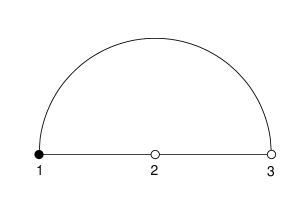
Figure 13: Particle-hole symmetry is broken by the particle’s preference to take the shortcut. A particle may move from site 1 to site 3, but a hole may not move from site 2 to site 1.

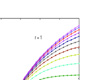
Figure 14: Plot of the current $J(\alpha)$ for fixed $\beta=1$ in the one-parameter family of models described in the text for $0\leq r\leq 1$ in a system of size $L=1024$. For $r=0$ only, the case of $1d$-TASEP, particle-hole symmetry is obeyed and phase transition into an MC phase occurs. For all $r>0$, the symmetry is broken and $J(\alpha)$ varies smoothly, similar to $r=1$, the case of HN3-TASEP.

VI Discussion

We found that there are many striking differences between $1d$-TASEP and TASEP on HN3. It is obvious that particle-hole symmetry is broken from the asymmetric phase diagram, where the phase boundary between HD and LD curves and favors a larger LD phase. The symmetry is broken due to the particle’s preference to take shortcuts, and Fig. 13 illustrates the most obvious case of this symmetry breaking. A particle may only move from site 1 to site 3, but a hole may not move from site 2 to site 1 since the particle may not move from site 1 to site 2. A full lattice with a single hole moving to the left cannot take every shortcut as does a single particle on an empty lattice moving to the right. The model favors the efficient flow of particles, and this is why the LD phase is larger and free flow persists for some values of $\alpha>\beta$.

Figure 15: Density $\rho$ (top) and current $J$ (bottom) of TASEP on HN3 with particles having 50% chance of only attempting long distance jump and 50% chance of only attempting jumps along the backbone.

The importance of this symmetry is highlighted by designing a one-parameter family of models that interprets between $1d$-TASEP and HN3-TASEP. In these models, particles attempt a long-range jump with probability $r$, $0\leq r\leq 1$. Should no jump result, either because no attempt was made or because the attempt failed, a nearest-neighbor jump is attempted. For $r=0$, only nearest-neighbor jumps occur, corresponding to $1d$-TASEP. In turn, for $r=1$, a long-range jump is always attempted first, as in HN3-TASEP. We can characterize the behavior of this model with $r$ sufficiently by presenting our numerical results for the current $J$ as a function of $\alpha$ for fixed $\beta=1$. Fig. 14 shows how the smooth variation of $J(\alpha)$ found for HN3-TASEP in Fig. 3 evolves from $r=1$ towards the $2nd$-order phase transition between LD and MC phases at $r=0$. Although finite-size effects (at $L=1024$ here) obscure the bend in $J$ at $\alpha=1/2$, it is quite clear that only for strictly $r=0$ there is a MC phase with a constant-current plateau. For any $r>0$, $J(\alpha)$ appears to remain a smooth function without the emergence of a plateau. Of course, for all such $r>0$, particle-hole symmetry is broken.

We can formulate an update rule on HN3 that does preserve particle-hole symmetry. For instance, the particle chosen for an update could attempt a long-range or a nearest-neighbor jump with probability $r$ and $1-r$, respectively, but not explore the alternative if such an attempt fails. Unfortunately, although $r=0$ again corresponds to $1d$-TASEP, $r=1$ does not attain HN3-TASEP but another version of $1d$-TASEP restricted to $\sim\sqrt{L}$ sites only. In Fig. 15 we display the density and the current as a function of $\alpha$ and $\beta$ for the case $r=1/2$. The symmetry with respect to $\alpha=\beta$ is easily visible. As in $1d$-TASEP, there are HD, LD, and MC phases with a shock line between HD and LD. The most notable differences are that $J>1/4$ in MC and the steep transitions in the density at each phase boundary.

Returning to HN3-TASEP, we found in the LD phase that the particles move freely across the lattice. As the injection rate $\alpha$ is increased, the density and current increase, and there are few collisions, but the network is still able to transport particles quickly. At the transition into the HD phase, jams snowball throughout the system and soon fill in the whole lattice. The shortcuts are likely to be blocked off and the particles slowly crawl along the backbone. One may make an analogy to vehicular traffic. Cars like particles can move along a one lane road, and they may not pass each other. They appear at the beginning of the road at a rate $\alpha$, and disappear at the end of the road at a rate $\beta.$ At some density of cars the average velocity drops significantly and the whole road is jammed. If we add highways then cars may enter a highway, go faster, and when they get off they end up in front of their peers. In free flowing traffic, highways reduce the amount of time for cars to reach their destination and lower the density, given the same boundary conditions. Traffic jams still occur with the addition of highways, and there are more possibilities for cars to maneuver around each other and fill in gaps so the density can be very high.

An interesting property of TASEP on HN3 is that the network uses mainly it’s long range connections to transport particles, and its backbone to ’store’ them. In the LD phase the particles flow freely through the highway. As $\alpha$ is increased, particles may be pushed into the less visited backbone sites, and the current and density increase. An inverse process happens in the HD phase, where as $\beta$ is increased more particles can be pulled from storage, the current goes up, and the density goes down. There is no possibility for the current and density to stay constant as both parameters are changed simultaneously, hence, there is no MC phase on HN3.

This storage mechanism could conceivably be useful in a real system. The transition between the HD and LD phases changes the system from very high density to very low density, while the current does not change significantly. Only a small local change in the rate of particle injection or removal at the boundaries can induce a dramatic global change in the number of particles. We have measure the effect of a protocol whereby at $\alpha=1$ the value of $\beta$ is switched between 0.7 (HD phase) and 0.8 (LD phase), see also Fig. 5. Unfortunately, it takes a long time, about a factor of 1000 longer than the typical transit time of a particle, to squeeze the excess particles through the single exit site, empty out the lattice and re-establish the steady state at $\beta=0.8$. In turn, jamming up the system by re-setting to $\beta=0.7$ attains it steady state at least an order of magnitude faster.

VII Conclusions

In this work we found that a variation of the TASEP with fixed long distance jumps can lead to significant changes in its phases, notably, the disappearance of the maximum current phase. This is surprising since the TASEP phases are considered to be robust to many changes. These changes were described qualitatively as a result of the particles velocity becoming essentially unbounded along paths utilizing the long jumps.

Despite the increased complexity of the rate equations for this model, the much-simplified phase structure we found allowed the possibility of an analytic approach that, even if approximate, should provide a good qualitative and quantitative description. While a more detailed solution eludes us here, it remains a worthwhile goal for the future, as it would provide novel insight into and control over a process that has stimulated significant advances in the understanding of non-equilibrium critical phenomena.

References

- [1] B. Schmittmann and R. K. P. Zia in Phase Transitions and Critical Phenomena, Vol. 17. (Academic Press, London), 1995.
- [2] C. T. MacDonald, J. H. Gibbs, and A. C. Pipkin. Biopolymers, 6:1, 1968.
- [3] A.-L. Barabasi and H. E. Stanley. Fractal Concepts in Surface Growth. Cambridge University Press, 1995.
- [4] O. Biham, A. A. Middleton, and D. Levine. Phys. Rev. A, 46:R6124, 1992.
- [5] K. Nagel and M. Schreckenberg. J. Phys. I France, 2:2221, 1992.
- [6] K. Nagel and M. Paczuski. Phys. Rev. E, 51:2909, 1995.
- [7] O. G. Berg, R. B. Winter, and P. H. von Hippel. Biochemistry, 20:6929, 1981.
- [8] B. Derrida, E. Domany, and D. Mukamel. J. Stat. Phys., 69:667, 1992.
- [9] B. Derrida, M. R. Evans, V. Hakim, and V. Pasquier. J. Phys. A: Math. Gen., 1493, 1993.
- [10] G. Schütz and E. Domany. J. Stat. Phys., 72:277, 1993.
- [11] H. Hinrichsen. Advances in Physics, 49:815, 2000.
- [12] M. Mobilia, T. Reichenbach, H. Hinsch, T. Franosch, and E. Frey. Banach Center Publications, 80:101, 2008.
- [13] J. Szavits-Nossan and K. Uzelac. Phys. Rev. E, 74, 051104, 2008.
- [14] S. Boettcher, B. Gonçalves, and H. Guclu. J. Phys. A: Math. Theor., 41:252001, 2008.
- [15] D. J. Watts and S. H. Strogatz. Nature, 393:440, 1998.
- [16] S. Boccaletti, V. Latora, Y. Moreno, M. Chavez, and D.-U. Hwang. Phys. Rep., 424:175, 2006.
- [17] S. Boettcher and B. Goncalves. Europhys. Lett., 84:30002, 2008.