Maps for general open quantum systems and a theory of linear quantum error correction

Abstract

We show that quantum subdynamics of an open quantum system can always be described by a Hermitian map, irrespective of the form of the initial total system state. Since the theory of quantum error correction was developed based on the assumption of completely positive (CP) maps, we present a generalized theory of linear quantum error correction, which applies to any linear map describing the open system evolution. In the physically relevant setting of Hermitian maps, we show that the CP-map based version of quantum error correction theory applies without modifications. However, we show that a more general scenario is also possible, where the recovery map is Hermitian but not CP. Since non-CP maps have non-positive matrices in their range, we provide a geometric characterization of the positivity domain of general linear maps. In particular, we show that this domain is convex, and that this implies a simple algorithm for finding its boundary.

I Introduction

The problem of the formulation and characterization of the dynamics of quantum open systems has a long and extensive history Davies:76 ; Alicki:87 ; Breuer:Book . This problem has become particularly relevant in the context of quantum information processing Nielsen:book , where a remarkable theory of quantum error correction (QEC) was developed in recent years to address the problem of how to process quantum information in the presence of decoherence and imperfect control Gaitan:book . A key assumption common to many previous QEC studies is that the evolution of the quantum information processor can be described by a succession of completely positive (CP) maps Kraus:83 , interrupted by unitary gates or measurements Knill:97b . However, it is well known that if the initial total system state is entangled, quantum dynamics is not described by a CP map Pechukas+Alicki:95 ; Stelmachovic:01 ; Jordan:04 ; Carteret:05 ; Rodriguez:07 . In fact, we showed very recently in Ref. ShabaniLidar:08 that a CP map arises if and only if the initial total system state has vanishing quantum discord Ollivier:01 , i.e., is purely classically correlated. One is thus naturally led to ask whether this impacts the applicability of QEC theory under circumstances where non-classical initial state correlations play a role. Here “initial state” does not refer exclusively to the “$t=0$” point, but also to intermediate times where the recovery map is applied, since this map was also assumed to be CP in standard quantum error correction theory Knill:97b . Motivated by this fact we here critically revisit the CP maps assumption in QEC, and show that it can be relaxed . To do so, we first consider the problem of characterizing the type of map that describes open system evolution given an arbitrary initial total system state (Section II). We show that this map is always a linear, Hermitian map (of which CP maps are a special case). We then argue that the generic noise map describing the evolution of a quantum computer as it undergoes fault tolerant quantum error correction (FT-QEC) is indeed not a CP map, but rather such a Hermitian, linear map (Section III). The reason is, essentially, that imperfect error correction results in residual non-classical correlations between the system and the bath, as the next QEC cycle is applied. To deal with this, we develop a generalized theory of QEC which we call “linear quantum error correction” (LQEC), which applies to arbitrary linear maps on the system (Section IV). Then we show that, fortunately, the CP-map based version of QEC theory applies without modifications in the physically relevant setting of Hermitian maps. However, we show that a more general scenario is also possible, where the recovery map is Hermitian but not CP. This is useful since it obviates the unrealistic assumption that the recovery ancillas enter the QEC cycle as classically correlated with the other system qubits. Our results significantly extend the realm of applicability of QEC, in particular to arbitrarily correlated system-environment states. We conclude in Section V.

II Quantum dynamical processes and maps

In this section we prove a basic new result, that a quantum dynamical process can always be represented as a linear, Hermitian map from the initial to the final system-only state. In doing so we rely heavily on our previous work ShabaniLidar:08 .

The dynamics of open quantum systems can be described as follows. Consider a quantum system $S$ coupled to another system $B$, with respective Hilbert spaces $\mathcal{H}_{S}$ and $\mathcal{H}_{B}$, such that together they form one isolated system, described by the joint initial state (density matrix) $\rho_{SB}(0)$. Their joint time-evolved state is then

$$\rho_{SB}(t)=U(t)\rho_{SB}(0)U^{{\dagger}}(t),$$ (1)

where $U(t)$ is the unitary propagator of the joint system-bath dynamics from the initial time $t=0$ to the final time $t$, i.e., the solution to the Schrodinger equation $\dot{U}=-(i/\hbar)[H,U]$, where $H$ is the joint system-bath Hamiltonian. The object of interest is the system $S$, whose state at all times $t$ is governed according to the standard quantum-mechanical prescription by the following quantum dynamical process (QDP):

$$\rho_{S}(t)=\mathrm{Tr}_{B}[\rho_{SB}(t)]=\mathrm{Tr}_{B}[U_{SB}(t)\rho_{SB}(0)U_{SB}(t)^{{\dagger}}].$$ (2)

$\mathrm{Tr}_{B}$ represents the partial trace operation, corresponding to an averaging over the bath degrees of freedom Breuer:Book .

The QDP (2) is a transformation from $\rho_{SB}(0)$ to $\rho_{S}(t)$. However, since we are not interested in the state of the bath, it is natural to ask:

Under which conditions on $\rho_{SB}(0)$ is the QDP a map $\Phi_{\mathrm{Q}}(t)$,

$$\rho_{S}(t)=\Phi_{\mathrm{Q}}(t)[\rho_{S}(0)],$$ (3)

and what are the properties of this map?

In general, a map is an association of elements in the range with elements in the domain. Here we use the term “map” solely to indicate a state-independent transformation between two copies of the same Hilbert space, in particular $\mathcal{H}_{S}\mapsto\mathcal{H}_{S}$. Then, a well-known partial answer is that if $\rho_{SB}(0)$ is a tensor product state, i.e., $\rho_{SB}(0)=\rho_{S}(0)\otimes\rho_{B}(0)$, then the QDP (2) is a CP map. A more general answer was provided in ShabaniLidar:08 . To explain this answer we must first introduce some terminology.

II.1 Various linear maps

A map $\Phi:\mathcal{B}(\mathcal{H})\mapsto\mathcal{B}(\mathcal{H})$ [space of bounded operators on $\mathcal{H}$] is linear if $\Phi[a\rho_{1}+b\rho_{2}]=a\Phi[\rho_{1}]+b\Phi[\rho_{2}]$ for any pair of states $\rho_{1},\rho_{2}:\mathcal{H}\mapsto\mathcal{H}$, and constants $a,b\in\mathbb{C}$. A linear map is called Hermitian if it maps all Hermitian operators in its domain to Hermitian operators. We first present an operator sum representation for arbitrary and Hermitian linear maps, that generalizes the standard Kraus representation for CP maps Kraus:83 . The proof is presented in Appendix A.

Theorem 1

A map $\Phi_{\mathrm{L}}:\mathfrak{M}_{n}\mapsto\mathfrak{M}_{m}$ (where $\mathfrak{M}_{n}$ is the space of $n\times n$ matrices) is linear iff it can be represented as

$$\Phi_{\mathrm{L}}(\rho)\text{ }=\sum\nolimits_{\alpha}E_{\alpha}\rho E_{\alpha}^{\prime\dagger}$$ (4)

where the “left and right operation elements” $\{E_{\alpha}\}$ and $\{E_{\alpha}^{\prime}\}$ are, respectively, $m\times n$ and $n\times m$ matrices.
$\Phi_{\mathrm{H}}$ is a Hermitian map iff

$$\Phi_{\mathrm{H}}(\rho)=\sum\nolimits_{\alpha}c_{\alpha}E_{\alpha}\rho E_{\alpha}^{\dagger},\quad c_{\alpha}\in\mathbb{R}.$$ (5)

We will sometimes denote a linear map by listing its elements, as in $\Phi_{\mathrm{L}}=\{E_{\alpha},E_{\alpha}^{\prime}\}_{\alpha=1}^{r}$. Note that a linear map $\Phi_{\mathrm{L}}=\{E_{\alpha},E_{\alpha}^{\prime}\}_{\alpha=1}^{r}$ is trace preserving if ${\sum_{\alpha=1}^{r}}E_{\alpha}^{\prime\dagger}E_{\alpha}=I$. Also note that the two sets of operation elements $\{E_{\alpha},E_{\alpha}^{\prime}\}_{i=1}^{r}$ and $\{F_{\beta},F_{\beta}^{\prime}\}_{\beta=1}^{r}$, where $F_{\beta}=\sum_{\alpha=1}^{r}u_{\alpha\beta}E_{\alpha}$ and $F_{\beta}^{\prime}=\sum_{\alpha=1}^{r}v_{\alpha\beta}E_{\alpha}^{\prime}$, represent the same linear map $\Phi_{\mathrm{L}}$ if the matrices $u$ and $v$ satisfy $uv^{{\dagger}}=I$.

As a simple example of a non-CP, Hermitian map, consider the inverse-phase-flip map. The well-known CP phase-flip map is Nielsen:book : $\Phi_{\mathrm{PF}}(\rho)=\mathcal{(}1-p)\rho+p\sigma_{z}\rho\sigma_{z}$, where $0\leq p\leq 1$ and $\sigma_{z}$ is a Pauli matrix. Solving for $\Phi_{\mathrm{PF}}^{-1}$ from $\Phi_{\mathrm{PF}}^{-1}[\Phi_{\mathrm{PF}}(\rho)]=\rho$, we find that $\Phi_{\mathrm{PF}}^{-1}(\rho)=c_{0}\rho+c_{1}\sigma_{z}\rho\sigma_{z}$, where $c_{1}=p/(2p-1)$ and $c_{0}=1-c_{1}$, and $c_{0},c_{1}$ have opposite sign for $0<p<1$. Moreover, $\mathrm{Tr}[\Phi_{\mathrm{PF}}^{-1}(\rho)]=\mathrm{Tr}(\rho)$. Therefore $\Phi_{\mathrm{PF}}^{-1}$ is a trace-preserving, Hermitian, non-CP map.

A linear map is called “completely positive” (CP) if it is a Hermitian map with $c_{\alpha}\geq 0$ $\forall\alpha$. CP maps play a key role in quantum information and quantum error correction Nielsen:book , though they have a much earlier origin Stinespring:55 ; Kraus:83 . There are other useful characterizations of CP maps – see, e.g., Refs. Breuer:Book ; Nielsen:book . It turns out that there is a tight connection between CP and Hermitian maps Jordan:04 ; Carteret:05 : a map is Hermitian iff it can be written as the difference of two CP maps.

The definition of a CP map $\Phi_{\mathrm{CP}}$ implies that it can be expressed in the Kraus operator sum representation Kraus:83 :

$$\rho_{S}(t)=\sum_{\alpha}E_{\alpha}(t)\rho_{S}(0)E_{\alpha}^{\dagger}(t)=\Phi_{\mathrm{CP}}(t)[\rho_{S}(0)].$$ (6)

If the operation elements $E_{\alpha}$ satisfy ${\sum_{\alpha}}E_{\alpha}^{\dagger}E_{\alpha}=I$ then $\mathrm{Tr}[\rho_{S}(t)]=1$.

II.2 Special linear states

Following Ref. ShabaniLidar:08 , we define the class of “special-linear” (SL) states for which the QDP (2) always results in a linear, Hermitian map. An arbitrary bipartite state on $\mathcal{H}_{S}\otimes\mathcal{H}_{B}$ can be written as

$$\rho_{SB}=\sum\nolimits_{ij}\varrho_{ij}|i\rangle\langle j|\otimes\phi_{ij},$$ (7)

where $\{|i\rangle\}_{i=1}^{\dim\mathcal{H}_{S}}$ is an orthonormal basis for $\mathcal{H}_{S}$, and $\{\phi_{ij}\}_{i,j=1}^{\dim\mathcal{H}_{S}}:\mathcal{H}_{B}\mapsto\mathcal{H}_{B}$ are normalized such that if $\mathrm{Tr}[\phi_{ij}]\neq 0$ then $\mathrm{Tr}[\phi_{ij}]=1$. The corresponding reduced system and bath states are then $\rho_{S}=\sum_{(i,j)\in\mathcal{C}}\varrho_{ij}|i\rangle\langle j|$, where $\mathcal{C}\equiv\{(i,j)|\mathrm{Tr}[\phi_{ij}]=1\}$, and $\rho_{B}(0)=\sum_{i}\varrho_{ii}\phi_{ii}$. Hermiticity and normalization of $\rho_{SB}$, $\rho_{S}$, and $\rho_{B}$ imply $\varrho_{ij}=\varrho_{ji}^{\ast}$, $\phi_{ij}=\phi_{ji}^{{\dagger}}$, and $\sum_{i}\varrho_{ii}=1$.

Definition 1

A bipartite state $\rho_{SB}$, parametrized as in Eq. (7), is in the SL-class if either $\mathrm{Tr}[\phi_{ij}]=1$ or $\phi_{ij}=0,$ $\forall i,j$.

Thus a non-SL state is a state for which there exist indexes $i$ and $j$ such that $\mathrm{Tr}[\phi_{ij}]=0$ but $\phi_{ij}\neq 0$. The following result proven in Ref. ShabaniLidar:08 (generalizing an earlier result in Ref. Rodriguez:07 ) provides an almost complete answer to the question posed above:

Theorem 2 (Theorem 2 of ShabaniLidar:08 )

If $\rho_{SB}(0)$ is an SL-class state then the QDP (2) is a linear, Hermitian map $\Phi_{\mathrm{H}}:\rho_{S}(0)\mapsto\rho_{S}(t)$.

A further result proven in Ref. ShabaniLidar:08 (Theorem 3 there) provides necessary and sufficient conditions on $\rho_{SB}(0)$ for the QDP (2) to be a CP map, namely, $\rho_{SB}(0)$ should be a state with vanishing quantum discord Ollivier:01 . Such a state cannot contain any quantum correlations. This clearly illustrates the limitations of CP maps in describing quantum dynamics. At the same time one may wonder as to the generality of the SL-class employed in Theorem 2. Non-SL states are sparse ShabaniLidar:08 , so it is in this regard that we stated that Theorem 2 provides an almost complete answer to the question posed above. However, we can go further. As mentioned without proof in Ref. ShabaniLidar:08 , in fact the QDP (2) is a linear, Hermitian map from $\rho_{S}(0)\mapsto\rho_{S}(t)$ for any initial state $\rho_{SB}(0)$. We next prove this key fact.

II.3 Hermitian maps for arbitrary initial states

We split the general initial state representation (7) into a sum over SL and non-SL terms (thus splitting $\{\varrho_{ij}\}$ and $\{\phi_{ij}\}$ into two sets):

$$\rho_{SB}(0)=\sum_{ij\in(\mathrm{SL})}\alpha_{ij}|i\rangle\langle j|\otimes\varphi_{ij}+\sum_{ij\in(\mathrm{nSL})}\beta_{ij}|i\rangle\langle j|\otimes\psi_{ij}.$$ (8)

In accordance with the definition of SL states, in the first sum we include only terms $\alpha_{ij}|i\rangle\langle j|\otimes\varphi_{ij}$ for which $\mathrm{Tr}[\varphi_{ij}]\neq 0$ or $\varphi_{ij}=0$, in the second only terms $\beta_{ij}|i\rangle\langle j|\otimes\psi_{ij}$ with bath operators $\{\psi_{ij}\}$ satisfying $\psi_{ij}\neq 0$ and $\mathrm{Tr}[\psi_{ij}]=0$. By virtue of this decomposition only the first term contributes to the initial system state: $\rho_{S}(0)=\mathrm{Tr}_{B}[\rho_{SB}(0)]=\sum_{ij(\mathrm{SL})}\alpha_{ij}|i\rangle\langle j|$. This is because the condition $\mathrm{Tr}[\psi_{ij}]=0$ eliminates any contribution from the second term in the decomposition (8) to the initial system state. Consequently Eq. (3) assumes an affine form:

$$\Phi_{\mathrm{Q}}(t)[\rho_{S}(0)]=\Phi_{\mathrm{SL}}(t)[\rho_{S}(0)]+K_{\mathrm{nSL}}(t),$$ (9)

with the term $K_{\mathrm{nSL}}(t)$ being a shift that is independent of $\rho_{S}(0)$.

As shown in Ref. ShabaniLidar:08 , the linear map $\Phi_{\mathrm{SL}}$ is constructed as a function of the bath operators $\{\varphi_{ij}\}$:

$$\Phi_{\mathrm{SL}}(t)[\rho_{S}(0)]\equiv\sum_{(i,j)\in(\mathrm{SL});k,\alpha}\lambda_{\alpha}^{ij}V_{kij}^{\alpha}P_{i}\rho_{S}(0)P_{j}(W_{kij}^{\alpha})^{{\dagger}},$$ (10)

where $P_{i}\equiv|i\rangle\langle i|$ are projectors, $\lambda_{\alpha}^{ij}$ are the singular values in the singular value decomposition $\phi_{ij}=\sum_{\alpha}\lambda_{\alpha}^{ij}|x_{ij}^{\alpha}\rangle\langle y_{ij}^{\alpha}|$, and the operators $V_{kij}^{\alpha}\equiv\langle\psi_{k}|U|x_{ij}^{\alpha}\rangle$ and $W_{kij}^{\alpha}\equiv\langle\psi_{k}|U|y_{ij}^{\alpha}\rangle$ act on the system only, with $\{|\psi_{k}\rangle\}$ being an orthonormal basis for the bath Hilbert space ${\mathcal{H}}_{B}$.

In addition, the non-SL terms in Eq.(8) generate the shift term

$$K_{\mathrm{nSL}}(t)=\sum_{ij\in(\mathrm{nSL})}\beta_{ij}\mathrm{Tr}_{B}[U_{SB}(t)|i\rangle\langle j|\otimes\psi_{ij}U_{SB}^{{\dagger}}(t)].$$ (11)

This shows explicitly that $K_{\mathrm{nSL}}(t)$ does not depend on the initial system state, since the latter is fully parametrized by the coefficients $\{\alpha_{ij}\}_{ij\in(\mathrm{SL})}$, while $K_{\mathrm{nSL}}(t)$ depends only upon the coefficients $\{\beta_{ij}\}_{ij\in(\mathrm{nSL})}$.

Now we take a further step to argue that the affine map (9) is actually a linear, Hermitian map if the map acts only on the space of density matrices. This is a direct application of the result in Ref. Jordan:04 .

Theorem 3

The QDP (2) is representable as a linear, Hermitian map $\Phi_{\mathrm{H}}(t):\rho_{S}(0)\mapsto\rho_{S}(t)$ for any initial system-bath state.

Proof. Let $N\equiv\dim\mathcal{H}_{S}$. Let $F_{0}\equiv I$ and let $\{F_{\mu}:\mathrm{Tr}(F_{\mu})=0\}_{\mu=1}^{N^{2}-1}$ be a basis for the set of traceless Hermitian matrices which are mutually orthogonal with respect to the Hilbert-Schmidt inner product, i.e., $\mathrm{Tr}(F_{\mu}F_{\nu})=N\delta_{\mu\upsilon}$. Hence the initial system state $\rho_{S}(0)$ can be expanded as

$$\rho_{S}(0)=\frac{1}{N}(I+\sum_{\mu=1}^{N^{2}-1}b_{\mu}F_{\mu});\quad b_{\mu}=\mathrm{Tr}[\rho_{S}(0)F_{\mu}]\equiv\langle F_{\mu}\rangle_{\rho_{S}(0)},$$ (12)

and the final system state is found to be

$$\rho_{S}(t) = \frac{1}{N}[\Phi_{\mathrm{SL}}(I)+\sum_{\mu=1}^{N^{2}-1}b_{\mu}\Phi_{\mathrm{SL}}(F_{\mu})]+K_{\mathrm{nSL}}$$ (13)

$$= \Phi_{\mathrm{H}}(t)[\rho_{S}(0)],$$

where the equivalent Hermitian map $\Phi_{\mathrm{H}}$ is constructed by setting $\Phi_{\mathrm{H}}(I)=\Phi_{\mathrm{SL}}(I)+NK_{\mathrm{nSL}}$ and $\Phi_{\mathrm{H}}(F_{\mu})=\Phi_{\mathrm{SL}}(F_{\mu})$ $1\leq\forall\mu\leq N^{2}-1$. That this map is Hermitian is simple to verify, for all the components are Hermitian.   

Theorem 3 provides a complete, and perhaps surprising answer to the question posed at the beginning of this section. Namely, the most general form of a quantum dynamical process, irrespective of the initial system-bath state (in particular arbitrarily entangled initial states are possible) is always reducible to a Hermitian map from the initial system to the final system state. The surprising aspect of this result is that it was not known previously whether QDP could always even be reduced to a map between system states.

Of course, this result does not resolve the more difficult question of ensuring the positivity of the final system state. That is, a Hermitian map may transform an initially positive system state to a non-positive one, violating the postulate of positivity of quantum states. To resolve this one must identify the “positivity domain” of $\Phi_{\mathrm{H}}$, i.e., the set of initial system states (positive by definition) which are mapped to positive states by $\Phi_{\mathrm{H}}$ Jordan:04 . We address this in the next subsection.

II.4 Geometric characterization of the Positivity Domain

In this subsection we prove the convexity of the positivity domain and propose a geometric method for characterizing it. Let $S(\mathcal{H})\equiv\{\rho\in\mathcal{L}(\mathcal{H}):\rho>0,\mathrm{Tr}\rho=1\}$, where $\mathcal{L}(\mathcal{H})$ is the set of all linear operators on $\mathcal{H}$. The positivity domain of a linear map $\Phi_{\mathrm{L}}:S(\mathcal{H})\mapsto\mathcal{B}(\mathcal{H})$ is: $P_{\Phi}\equiv\{\rho\in S(\mathcal{H}_{S}):\Phi_{\mathrm{L}}(\rho)>0\}$.

Following earlier work Jakobczyk:01 ; Kimura:03 ; byrd:062322 , in Ref. Kimura:05 , a complete geometric characterization of density matrices was given by using the Bloch vector representation for an arbitrary $N$-dimensional Hilbert space $\mathcal{H}$. This works as follows: let $\{F_{\mu}\}_{\mu=1}^{N^{2}-1}$ be a basis set as in the proof of Theorem 3, whence the expansion (12) applies again. The vector $\mathbf{b}=(b_{1},...,b_{N^{2}-1})\in\mathbb{R}^{N^{2}-1}$ of expectation values is known as the Bloch vector, and knowing its components is equivalent to complete knowledge of the corresponding density matrix, via the map $\mathbf{b}\mapsto\rho\mathbf{=}\frac{1}{N}(I+\sum_{\mu=1}^{N^{2}-1}b_{\mu}F_{\mu})$. Let $\mathbf{n}$ denote a unit vector, i.e., $\mathbf{n}\in\mathbb{R}^{N^{2}-1}$ and $\sum_{i=1}^{N^{2}-1}n_{i}^{2}=1$, and define $F_{\mathbf{n}}\equiv\sum_{\mu=1}^{N^{2}-1}n_{\mu}F_{\mu}$. Let the minimum eigenvalue of each $F_{\mathbf{n}}$ be denoted $m(F_{\mathbf{n}})$. The “Bloch space” $\boldsymbol{B}(\mathbb{R}^{N^{2}-1})$ is the set of all Bloch vectors and is a closed convex set, since the set $S(\mathcal{H})$ is closed and convex, and the map $\mathbf{b}\mapsto\rho$ is linear homeomorphic. As shown in Theorem 1 of Ref. Kimura:05 , the Bloch space is characterized in the “spherical coordinates” determined by $\{F_{\mathbf{n}}\}$ as:

$$\boldsymbol{B}(\mathbb{R}^{N^{2}-1})=\left\{\mathbf{b}=r\mathbf{n}\in\mathbb{R}^{N^{2}-1}:r\leq\frac{1}{|m(F_{\mathbf{n}})|}\right\}.$$ (14)

It is hard to imagine a more intuitive or simpler geometric picture.

Next we show that the positivity domain is a convex set as well.

Proposition 1

The positivity domain $P_{\Phi}$ of a linear map $\Phi_{\mathrm{L}}$ is a convex set.

Proof. Consider two density matrices $\rho$ and $\rho^{\prime}$ as interior points of $P_{\Phi}$ with corresponding Bloch vectors $\mathbf{b}=(b_{1},...,b_{N^{2}-1})$ and $\mathbf{b^{\prime}}=(b_{1}^{\prime},...,b_{N^{2}-1}^{\prime})$. The claim is that a third density matrix $\rho^{\prime\prime}$ with corresponding Bloch vector $\mathbf{b^{\prime\prime}}(\alpha)=\alpha\mathbf{b}+(1-\alpha)\mathbf{b^{\prime}}$, with $0\leq\alpha\leq 1$, is then also interior to $P_{\Phi}$. This follows directly by linearity of the map $\Phi_{\mathrm{L}}$. First, by assumption $\Phi_{\mathrm{L}}[\rho]=\Phi_{\mathrm{L}}[\frac{1}{N}(I+\sum_{\mu=1}^{N^{2}-1}b_{\mu}F_{\mu})]>0$ and $\Phi_{\mathrm{L}}[\rho^{\prime}]=\Phi_{\mathrm{L}}[\frac{1}{N}(I+\sum_{\mu=1}^{N^{2}-1}b_{\mu}^{\prime}F_{\mu})]>0$, so that $\alpha\Phi_{\mathrm{L}}[\rho]+(1-\alpha)\Phi_{\mathrm{L}}[\rho^{\prime}]>0$. Second, $\alpha\Phi_{\mathrm{L}}[\rho]+(1-\alpha)\Phi_{\mathrm{L}}[\rho^{\prime}]=\Phi_{\mathrm{L}}[\frac{1}{N}I]+\alpha\sum_{\mu=1}^{N^{2}-1}b_{\mu}\Phi_{\mathrm{L}}[F_{\mu}]+(1-\alpha)\sum_{\mu=1}^{N^{2}-1}b_{\mu}^{\prime}\Phi_{\mathrm{L}}[F_{\mu}]=\Phi_{\mathrm{L}}[\frac{1}{N}(I+\sum_{\mu=1}^{N^{2}-1}b_{\mu}^{\prime\prime}F_{\mu})]=\Phi_{\mathrm{L}}[\rho^{\prime\prime}]$. Therefore indeed $\Phi_{\mathrm{L}}[\rho^{\prime\prime}]>0$.   

We are now ready to describe an algorithm for finding the boundary of the positivity domain $P_{\Phi}$. We know at this point that $P_{\Phi}$ is convex and that $P_{\Phi}$ is a subset of the Bloch space, itself a closed convex set. Pick a unit vector $\mathbf{n}$ and draw a line through the origin of the Bloch space along $\mathbf{n}$. If $P_{\Phi}$ includes the origin, i.e., the maximally mixed state, then convexity implies that this line intersects the boundary of $P_{\Phi}$ once. If $P_{\Phi}$ does not include the origin then convexity implies that this line either intersects the boundary of $P_{\Phi}$ twice or not at all. I.e., it follows from convexity that the line may not re-enter the positivity domain once it exited. In order to determine this boundary we may thus compute the eigenvalues of $\Phi_{\mathrm{L}}[\rho_{\mathbf{n}}(r)]$ as a function of $r$, where $r$ is the parameter in Eq. (14), and where $\rho_{\mathbf{n}}(r)$ is the density matrix determined via the mapping $\mathbf{b}=r\mathbf{n}\mapsto\rho$. The computation should start from $r=0$ and go up to at most $r=1/|m(F_{\mathbf{n}})|$. The boundary is identified as soon as the eigenvalues of $\Phi_{\mathrm{L}}[\rho_{\mathbf{n}}(r)]$ go from all positive semi-definite to at least one negative, or vice versa. For each unit vector $\mathbf{n}$, the corresponding point on the border of the positivity domain can be found in this way. Then the algorithm constructs the boundary of the positivity domain by finding the boundary points in all directions $\mathbf{n}$. Of course, in practice one can only sample the space of unit vectors $\mathbf{n}$ and factors $r$. In principle this yields a complete geometrical description of the positivity domain of a given linear map.

III CP maps and fault tolerant quantum error correction

III.1 CP maps: pro and con

We have already mentioned that a QDP (2) becomes a CP map iff the initial system-bath state has vanishing quantum discord, i.e., is purely classically correlated ShabaniLidar:08 . The standard argument in favor of CP maps is that since the system $S$ may be coupled with the bath $B$, the maps describing physical processes on $S$ should be such that all their extensions into higher dimensional spaces should remain positive, i.e., $\Phi_{\mathrm{CP}}\otimes I_{n}\geq 0$ $\forall n\in\mathbb{Z}^{+}$, where $I_{n}$ is the $n$-dimensional identity operator. However, one may question whether this is the right criterion for describing quantum dynamics Pechukas+Alicki:95 . An alternative viewpoint is to seek a description that applies to arbitrary $\rho_{SB}(0)$, as we have done above. We now argue that this viewpoint is the correct one for fault-tolerant quantum error correction (FT-QEC).

III.2 (In)validity of the CP map model in FT-QEC

Let us show that system-environment correlations impose a severe restriction on the applicability of CP maps in FT-QEC. The CP map model used in FT-QEC Shor:96 ; Aharonov:96 ; Knill:98 ; Steane:03 ; Knill:05 ; Reichardt:05 ; Aharonov:08 ; Aliferis:08 can be described as follows (see, e.g., Eq. (8.1) in Aharonov:08 ): $\rho_{S}(T)=\Phi_{\mathrm{CP}}^{\mathrm{tot}}(T,t_{0})[\rho_{S}(t_{0})]$ where

$$\Phi_{\mathrm{CP}}^{\mathrm{tot}}(T,t_{0})=\bigotimes\nolimits_{i=1}^{N}\Phi_{U}(t_{i})\Phi_{\mathrm{CP}}(t_{i},t_{i-1}),$$ (15)

where $T\equiv t_{N}$ is the total circuit time, and where $\Phi_{U}[\rho_{S}]=U_{S}\rho_{S}U_{S}^{\dagger}$ is a unitary map (automatically CP) that describes an ideal quantum logic gate. This represents the idea used repeatedly in FT-QEC, that the noisy evolution at every time step can be decomposed into “pure noise” $\Phi_{\mathrm{CP}}(t_{i},t_{i-1})$ followed by an instantaneous and perfect unitary gate $\Phi_{U}(t_{i})$. More precisely, in FT-QEC one assumes that the evolution starts ($t=t_{0}=0$) from a product state, then undergoes a CP map $\Phi_{\mathrm{CP}}(t_{1},t_{0})$ due to coupling to the environment, followed by an instantaneous error correction step $\Phi_{U}(t_{1})$. If the latter were perfect then the post-error-correction state would again be a product state $\rho_{S}(t_{1})\otimes\rho_{B}(t_{1})$. However, FT-QEC allows for the fact that the error correction step is almost never perfect, which means that there is a residual correlation between system and bath at $t_{1}$. Hence, according to Ref. ShabaniLidar:08 , the map that describes the evolution of the system is a CP map if and only if the residual correlation is purely classical. Otherwise it is a Hermitian map. To make this point more explicit, consider a sequence of two noise time-steps, interrupted by one error correction step. In the ideal scenario, where the error correction step $\Phi_{U}(t_{1})$ works perfectly (i.e., reduces the system-bath correlations to purely classical), we would have

$$\Phi_{\mathrm{CP}}^{\mathrm{(2)}}(t_{2},t_{0})=\Phi_{\mathrm{CP}}(t_{2},t_{1})\Phi_{U}(t_{1})\Phi_{\mathrm{CP}}(t_{1},t_{0}),$$ (16)

where $\Phi_{\mathrm{CP}}(t_{2},t_{1})$ is again a CP noise map. However, in reality $\Phi_{U}(t_{1})$ works imperfectly [system-bath correlations are not purely classical after the action of $\Phi_{U}(t_{1})$], and the actual map obtained is

$$\Phi_{\mathrm{H}}^{\mathrm{(2)}}(t_{2},t_{0})=\Phi_{\mathrm{H}}(t_{2},t_{1})\Phi_{U}(t_{1})\Phi_{\mathrm{CP}}(t_{1},t_{0}),$$ (17)

where $\Phi_{\mathrm{H}}(t_{2},t_{1})$ is now a Hermitian map. Note that, in fact, even the assumption that the first noise map is CP will not be true in general, due to errors in the preparation of the initial state, leading to non-classical correlations between system and bath. We conclude that in general the CP map model (15) should be replaced by

$$\Phi_{\mathrm{H}}^{\mathrm{tot}}(T,t_{0})=\bigotimes\nolimits_{i=1}^{N}\Phi_{U}(t_{i})\Phi_{\mathrm{H}}(t_{i},t_{i-1}),$$ (18)

where $\Phi_{\mathrm{H}}(t_{i},t_{i-1})$ are Hermitian maps, not necessarily CP.

It is worth emphasizing that this distinction between purely classical and other correlations, and the resulting difference between CP and Hermitian evolution, is not a distinction that has thus far been made in FT-QEC theory. Rather, in FT-QEC one distinguishes between “good” and “bad” fault paths, where the former (latter) contain only a few (too many) errors. Quoting from Terhal:04 : “There are good fault paths with so-called sparse numbers of faults which keep being corrected during the computation and which lead to (approximately) correct answers of the computation; and there are bad fault-paths which contain too many faults to be corrected and imply a crash of the quantum computer.” This leads to a splitting of the total map (15) into a sum over good and bad paths. One then shows that the computation can proceed robustly via the use of concatenated codes, provided the “bad” paths are appropriately bounded. In Aharonov:08 (p.1272) it was pointed out that the sum over “good” paths need not be a CP map, but can be decomposed into a new sum over CP maps [Eq. (8.13) there]. This new decomposition can then be treated using standard FT-QEC techniques. However, this assumes again that the total evolution is a CP map, which in fact it is not [Eq. (18)].

These observations motivate a generalized theory of QEC, which can handle non-CP noise maps. This is the subject of the next section. The main result of this theory is reassuring: in spite of the invalidity of the CP map model in FT-QEC, the CP-map based results apply because the same encoding and recovery that corrects a Hermitian map can be used to correct a closely related CP map, whose coefficients are the absolute values of the Hermitian map. This is formalized in Corollary 1.

IV Linear Quantum Error Correction

Having argued that non-CP Hermitian maps arise naturally in the study of open systems, and in particular FT-QEC, we now proceed to develop the theory of Linear QEC. For generality we do this for arbitrary linear maps, i.e., maps of the form (4). We then specialize to the physically relevant case of Hermitian maps.

Let us first recall the fundamental theorem of “standard” QEC (for CP noise and CP recovery maps) Knill:97b : Let $P$ be a projection operator onto the code space. Necessary and sufficient conditions for quantum error correction of a CP map, $\Phi_{\mathrm{CP}}(\rho)={\sum_{i}}F_{i}\rho F_{i}^{\dagger}$ are

$$PF_{i}^{{\dagger}}F_{j}P=\lambda_{ij}P\quad\forall i,j.$$ (19)

An elegant proof of this theorem and a construction of the corresponding CP recovery map was given in Refs. Nielsen:98 ; Nielsen:book ; we use some of their methods in the proofs of Theorems 4,5.

IV.1 CP-recoverable linear noise maps

While general (non-Hermitian) linear maps of the form (4) do not arise from quantum dynamical processes [Eq. (2)], it is still interesting from a purely mathematical standpoint to consider QEC for such maps. Moreover, we easily recover the physical setting from these general considerations.

Theorem 4 shows that there is a class of linear noise maps which are equivalent to certain non-trace-preserving CP noise maps when it comes to error correction using CP recovery maps.

Theorem 4

Consider a general linear noise map $\Phi_{\mathrm{L}}(\rho)$ $={\sum_{i=1}^{N}}E_{i}\rho E_{i}^{\prime\dagger}$ and associate to it an “expanded” CP map $\tilde{\Phi}_{\mathrm{CP}}(\rho)=\frac{1}{2}{\sum_{i=1}^{N}}E_{i}\rho E_{i}^{\dagger}+\frac{1}{2}{\sum_{i=1}^{N}}E_{i}^{\prime}\rho E_{i}^{\prime\dagger}$. Then any QEC code $\mathcal{C}$ and corresponding CP recovery map $\mathcal{R}$ for $\tilde{\Phi}_{\mathrm{CP}}$ are also a QEC code and CP recovery map for $\Phi_{\mathrm{L}}$.

Proof. The operation elements of $\tilde{\Phi}_{\mathrm{CP}}$ are $\{F_{i}\}_{i=1}^{N}=\{\frac{1}{\sqrt{2}}E_{i}\}_{i=1}^{N}$ and $\{F_{N+i}\}_{i=1}^{N}=\{\frac{1}{\sqrt{2}}E_{i}^{\prime}\}_{i=1}^{N}$, whence $\tilde{\Phi}_{\mathrm{CP}}(\rho)={\sum_{i=1}^{2N}}F_{i}\rho F_{i}^{\dagger}$. The standard quantum error correction conditions (19) for $\tilde{\Phi}_{\mathrm{CP}}$, where

$$\lambda\equiv 2\left(\begin{array}[]{cc}\alpha&\gamma\\ \gamma^{{\dagger}}&\alpha^{\prime}\end{array}\right)=\lambda^{{\dagger}},$$ (20)

become three sets of conditions in terms of the $E_{i}$ and $E_{i}^{\prime}$:

$$\text{(i)}~{}PE_{i}^{{\dagger}}E_{j}P = 2\alpha_{ij}P,~{}\text{(ii)}~{}PE_{i}^{\prime{\dagger}}E_{j}^{\prime}P=2\alpha_{ij}^{\prime}P,$$

$$\text{(iii)}~{}PE_{i}^{{\dagger}}E_{j}^{\prime}P = 2\gamma_{ij}P,$$ (21)

where $i,j\in\{1,...,N\}$ and $\alpha_{ij}=\lambda_{ij}$, $\gamma_{ij}=\lambda_{i,N+j}$, $\alpha_{ij}^{{}^{\prime}}=\lambda_{N+i,N+j}$. The existence of a projector $P$ which satisfies Eqs. (21)(i)-(iii) is equivalent to the existence of a QEC code for $\tilde{\Phi}_{\mathrm{CP}}$. Assuming that a code $\mathcal{C}$ has been found (i.e., $P\mathcal{C}=\mathcal{C}$) for $\tilde{\Phi}_{\mathrm{CP}}$, we use this as a code for $\Phi_{\mathrm{L}}$ and show that the corresponding CP recovery map $\mathcal{R}_{\mathrm{CP}}$ is also a recovery map for $\Phi_{\mathrm{L}}$. Indeed, let $G_{j}\equiv\sum_{i=1}^{2N}u_{ij}F_{i}$ be new operation elements for $\tilde{\Phi}_{\mathrm{CP}}$, where $u$ is the unitary matrix that diagonalizes $\lambda$, i.e., $u^{{\dagger}}\lambda u=d$. Then $\tilde{\Phi}_{\mathrm{CP}}={\sum_{j=1}^{2N}}G_{j}\rho G_{j}^{\dagger}$. Let $\mathcal{R}_{\mathrm{CP}}=\{R_{k}\}$ be the CP recovery map for $\tilde{\Phi}_{\mathrm{CP}}$. Assume that $\rho$ is in the code space, i.e., $P\rho P=\rho$. We now show that $\mathcal{R}_{\mathrm{CP}}[\Phi_{\mathrm{L}}(\rho)]=\rho$, i.e., we have CP recovery. First,

$$\mathcal{R}_{\mathrm{CP}}[\Phi_{\mathrm{L}}(\rho)] = \sum_{k}R_{k}\left(\sum_{i=1}^{N}F_{i}\rho F_{N+i}^{{\dagger}}\right)R_{k}^{{\dagger}}$$ (22)

$$= \sum_{i=1}^{N}\sum_{j,j^{\prime}=1}^{2N}u_{ij}^{\ast}u_{N+i,j^{\prime}}\times$$

$$\sum_{k}\left(R_{k}G_{j}P\right)\rho\left(PG_{j^{\prime}}^{{\dagger}}R_{k}^{{\dagger}}\right).$$

Now, note that

$$PG_{k}^{{\dagger}}G_{l}P = \sum_{ij}u_{ik}^{\ast}u_{jl}PF_{i}^{{\dagger}}F_{j}P=\sum_{ij}u_{ik}^{\ast}\lambda_{ij}u_{jl}P$$ (23)

$$= d_{k}\delta_{kl}P.$$

Then the polar decomposition yields

$$G_{k}P=U_{k}(PG_{k}^{{\dagger}}G_{k}P)^{1/2}=\sqrt{d_{k}}U_{k}P.$$ (24)

The recovery operation elements are given by

$$R_{k}=U_{k}^{{\dagger}}P_{k},$$ (25)

where $P_{k}=U_{k}PU_{k}^{{\dagger}}$. Therefore $P_{k}=G_{k}PU_{k}^{{\dagger}}/\sqrt{d_{k}}$. This allows us to calculate the action of the $k$th recovery operator on the $l$th error Nielsen:98 ; Nielsen:book :

$$R_{k}G_{l}P = U_{k}^{{\dagger}}P_{k}^{{\dagger}}G_{l}P=U_{k}^{{\dagger}}(U_{k}PG_{k}^{{\dagger}}/\sqrt{d_{k}})G_{l}P$$ (26)

$$= \delta_{kl}\sqrt{d_{k}}P.$$

Therefore,

$$\mathcal{R}_{\mathrm{CP}}[\Phi_{\mathrm{L}}(\rho)] = \sum_{i=1}^{N}\sum_{j,j^{\prime}=1}^{2N}u_{ij}^{\ast}u_{N+i,j^{\prime}}$$ (27)

$$\times\sum_{k}\left(\delta_{kj}\sqrt{d_{k}}P\right)\rho\left(P\sqrt{d_{k}}\delta_{kj^{\prime}}\right)$$

$$= \rho\sum_{i=1}^{N}\left(udu^{{\dagger}}\right)_{N+i,i}=\rho\sum_{i=1}^{N}\lambda_{N+i,i}$$

$$= 2\rho\mathrm{Tr}\gamma^{{\dagger}}.$$

Next note that, using condition (21)(iii) and trace preservation by $\Phi_{\mathrm{L}}$:

$$PE_{i}^{\prime{\dagger}}E_{i}P = 2\gamma_{ii}^{{\dagger}}P\Longrightarrow 2\mathrm{Tr}\gamma^{{\dagger}}P=P\sum_{i}E_{i}^{\prime{\dagger}}E_{i}P=P$$ (28)

$$\Longrightarrow \mathrm{Tr}\gamma^{{\dagger}}=\frac{1}{2}.$$

Hence, finally:

$$\mathcal{R}_{\mathrm{CP}}[\Phi_{\mathrm{L}}(\rho)]=\rho$$ (29)

for any $\rho$ in the codespace.   

Note that $\tilde{\Phi}_{\mathrm{CP}}(\rho)$ need not be trace preserving:$\ \mathrm{Tr}[\tilde{\Phi}_{\mathrm{CP}}(\rho)]=\frac{1}{2}\mathrm{Tr}[({\sum_{i=1}^{N}}E_{i}^{\dagger}E_{i}+{\sum_{i=1}^{N}}E_{i}^{\prime\dagger}E_{i}^{\prime})\rho]$, and while ${\sum_{i=1}^{N}}E_{i}^{\prime\dagger}E_{i}=I$ if $\Phi_{\mathrm{L}}$ is trace preserving, we do not have conditions on ${\sum_{i=1}^{N}}E_{i}^{\dagger}E_{i}$ and ${\sum_{i=1}^{N}}E_{i}^{\prime\dagger}E_{i}^{\prime}$.

We define the class of “CP-recoverable linear noise maps” $\{\Phi_{\mathrm{CPR}}\}$ as those $\Phi_{\mathrm{L}}$ for which CP recovery is always possible. By Theorem 4 this includes all $\Phi_{\mathrm{L}}$ for which $P$ can be found satisfying conditions (21)(i)-(iii). However, these conditions are not necessary.

IV.2 Non-CP-recoverable linear noise maps

We now define “non-CP-recoverable linear noise maps” $\{\Phi_{\mathrm{nCPR}}\}$ as those $\Phi_{\mathrm{L}}$ for which non-CP-recovery is always possible. Theorem 5 shows constructively that $\{\Phi_{\mathrm{nCPR}}\}$ includes all linear noise maps $\Phi_{\mathrm{L}}$ for which $P$ can be found satisfying only conditions (21)(i) and (ii). Clearly, $\{\Phi_{\mathrm{CP}}\}\subset\{\Phi_{\mathrm{CPR}}\}\subset\{\Phi_{\mathrm{nCPR}}\}\subset\{\Phi_{\mathrm{L}}\}$.

Theorem 5

Let $\Phi_{\mathrm{L}}=\{E_{i},E_{i}^{\prime}\}_{i}$ be a linear noise map. Then every state $\rho=P\rho P$ encoded using a QEC code defined by a projector $P$ satisfying only Eqs. (21)(i) and (ii) can be recovered using a non-CP recovery map.

Proof. Let $G_{k}=\sum_{i}u_{ik}E_{i}$ and $G_{k}^{\prime}=\sum_{i}u_{ik}^{\prime}E_{i}^{\prime}$, where the unitaries $u$ and $u^{\prime}$ respectively diagonalize the Hermitian matrices $\alpha$ and $\alpha^{\prime}$: $d=u^{{\dagger}}\alpha u$ and $d^{\prime}=u^{\prime{\dagger}}\alpha^{\prime}u^{\prime}$. Define a recovery map $\mathcal{R}=\{R_{k},R_{k}^{\prime}\}$ (not necessarily CP) with operation elements

$$R_{k}=U_{k}^{{\dagger}}P_{k},\quad R_{k}^{\prime}=U_{k}^{\prime{\dagger}}P_{k}^{\prime}.$$ (30)

Here $P_{k}=U_{k}PU_{k}^{{\dagger}}$, $P_{k}^{\prime}=U_{k}^{\prime}PU_{k}^{\prime{\dagger}}$ are projection operators, and $U_{k}$ and $U_{k}^{\prime}$ arise from the polar decomposition of $G_{k}P$ and $G_{k}^{\prime}P$, i.e., $G_{k}P=U_{k}(PG_{k}^{{\dagger}}G_{k}P)^{1/2}$ and $G_{k}^{\prime}P=U_{k}(PG_{k}^{\prime{\dagger}}G_{k}^{\prime}P)^{1/2}$. The proof is entirely analogous to the proof of Theorem 4, except that we must keep track of both the primed and unprimed operators. Following through the same calculations we thus obtain $R_{k}G_{l}\sqrt{\rho}=\sqrt{d_{k}}\delta_{kl}\sqrt{\rho}$ and $R_{k}^{\prime}G_{l}^{\prime}\sqrt{\rho}=\sqrt{d_{k}^{\prime}}\delta_{kl}\sqrt{\rho}$. Using this in the recovery map applied to the linear noise map, we find:

$$\mathcal{R}[\Phi(P\rho P)] = \sum_{kl}R_{k}E_{l}P\rho PE_{l}^{\prime\dagger}R_{k}^{\prime{\dagger}}$$ (31)

$$= \sum_{kl}R_{k}(\sum_{j}u_{lj}^{\ast}G_{j})P\rho P(\sum_{i}u_{li}^{\prime}G_{i}^{\prime{\dagger}})R_{k}^{\prime{\dagger}}$$

$$= F_{\mathrm{L}}P\rho P\propto\rho,$$

where

$$F_{\mathrm{L}} \equiv \sum_{ijkl}u_{lj}^{\ast}u_{li}^{\prime}\sqrt{d_{k}d_{k}^{\prime\ast}}\delta_{kj}\delta_{ki}=\sum_{kl}u_{lk}^{\ast}u_{lk}^{\prime}\sqrt{d_{k}d_{k}^{\prime\ast}}$$ (32)

$$= \mathrm{Tr}[u^{\prime}d^{\prime{\dagger}}du^{{\dagger}}]=\mathrm{Tr}[u^{\prime}u^{{\dagger}}\alpha\alpha^{\prime{\dagger}}]$$

is a “correction factor” for non-CP recovery of linear noise maps, which was $1$ in the case of CP recovery, above.   

Gathering the expressions derived in the last proof, we have the following explicit expressions for the left and right recovery operations:

$$R_{k}=U_{k}^{{\dagger}}P_{k}^{{\dagger}}=\frac{1}{\sqrt{d_{k}}}P\sum_{i}u_{ik}^{\ast}E_{i}^{{\dagger}},~{}R_{k}^{\prime}=\frac{1}{\sqrt{d_{k}^{\prime}}}P\sum_{i}u_{ik}^{\prime\ast}E_{i}^{\prime{\dagger}}.$$ (33)

This also shows that, in general, $R_{k}$ need not equal $R_{k}^{\prime}$, i.e., the recovery map is linear but not necessarily CP.

Note that standard QEC can also be interpreted as “error correction by inversion”, in the following sense: when the noise map is CP and recovery is also CP, recovery is the inverse of the noise map restricted to the code space (Theorem III.3 in Ref. Knill:97b ). The same is true for our LQEC results above, which relax the restriction to CP noise maps.

IV.3 The physical case: Hermitian maps

The general physical case is the case of Hermitian noise maps, to which any quantum dynamical process can be reduced, as follows from Theorem 3. We can specialize Theorems 4 and 5 to this case.

Corollary 1

Consider a Hermitian noise map $\Phi_{\mathrm{H}}(\rho)$ $={\sum_{i=1}^{N}}c_{i}K_{i}\rho K_{i}^{\dagger}$ and associate to it a CP map $\tilde{\Phi}_{\mathrm{CP}}(\rho)={\sum_{i=1}^{N}|}c_{i}|K_{i}\rho K_{i}^{\dagger}$. Then any QEC code $\mathcal{C}$ and corresponding CP recovery map $\mathcal{R}_{\mathrm{CP}}$ for $\tilde{\Phi}_{\mathrm{CP}}$ are also a QEC code and CP recovery map for $\Phi_{\mathrm{H}}$.

The important conclusion we can draw from Corollary 1 is that standard QEC techniques apply whether the noise map is CP or, as it will almost always be due to non-classical correlations, Hermitian. This is because Corollary 1 tells us that it is safe to replace all negative $c_{i}$ coefficients by their absolute values, and thus replace the actual noise map by its CP counterpart.

Proof. We have $\Phi_{\mathrm{H}}(\rho)={\sum_{i=1}^{N}}E_{i}\rho E_{i}^{\prime\dagger}$ with $\{{E}_{i}=\sqrt{c_{i}}K_{i}\}_{i=1}^{N}$ and $\{{E}_{i}^{\prime}=(\sqrt{c_{i}})^{\ast}K_{i}\}_{i=1}^{N}$, whence we can apply the construction of Theorem 4. Indeed, the “expanded” CP map becomes $\tilde{\Phi}_{\mathrm{CP}}(\rho)=\frac{1}{2}{\sum_{i=1}^{N}}E_{i}\rho E_{i}^{\dagger}+\frac{1}{2}{\sum_{i=1}^{N}}E_{i}^{\prime}\rho E_{i}^{\prime\dagger}={\sum_{i=1}^{N}|}c_{i}|K_{i}\rho K_{i}^{\dagger}$, as claimed, and hence a QEC code and CP recovery for $\tilde{\Phi}_{\mathrm{CP}}$ is also a QEC code and CP recovery for $\Phi_{\mathrm{H}}$. In particular, $\mathcal{R}_{\mathrm{CP}}[\Phi_{\mathrm{H}}(\rho)]=\rho$.   

Note that $\tilde{\Phi}_{\mathrm{CP}}$ need not be trace preserving even in the Hermitian map case: $\mathrm{Tr}[\tilde{\Phi}_{\mathrm{CP}}(\rho)]=\mathrm{Tr}[{\sum_{i=1}^{N}|}c_{i}|K_{i}^{\dagger}K_{i}\rho]$, but if $\Phi_{\mathrm{H}}$ is trace preserving then we only have ${\sum_{i=1}^{N}}c_{i}K_{i}^{\dagger}K_{i}=I$, hence cannot conclude more about $\mathrm{Tr}[\tilde{\Phi}_{\mathrm{CP}}(\rho)]$. Also note that substitution of ${E}_{i}=\sqrt{c_{i}}K_{i}$ and ${E}_{i}^{\prime}=(\sqrt{c_{i}})^{\ast}K_{i}$ into the QEC conditions (21)(i)-(iii) yields $\alpha_{ij}^{\prime}=\sqrt{\frac{c_{i}}{c_{j}}}\left(\sqrt{\frac{c_{j}}{c_{i}}}\right)^{\ast}\alpha_{ij}$ and $\gamma_{ij}=\frac{(\sqrt{c_{j}})^{\ast}}{\sqrt{c_{j}}}\alpha_{ij}$, i.e., unlike in the general linear maps case, the matrices $\alpha^{\prime}$ and $\gamma$ in Eq. (20) are not independent from $\alpha$. In fact, as shown in Appendix B we can give a direct proof of Corollary 1 which only invokes a single block of the $\lambda$ matrix.

IV.3.1 Example of CP recovery: Inverse bit-flip map

Consider “diagonalizable maps”, i.e., $\Phi_{\mathrm{D}}(\rho)\equiv\sum_{i}c_{i}K_{i}\rho K_{i}^{\dagger}$, where $c_{i}\in\mathbb{C}$. The expanded CP map is $\tilde{\Phi}_{\mathrm{CP}}=\sum_{i}|c_{i}|K_{i}\rho K_{i}^{\dagger}$. Now consider as a specific instance an independent-errors inverse bit-flip map on three qubits: $\Phi_{\mathrm{IPF}}(\rho)=c_{0}\rho+c_{1}\sum_{n=1}^{3}X_{n}\rho X_{n}$, where $X_{n}$ is the Pauli $\sigma_{x}$ matrix applied to qubit $n$, where $c_{0}$ and $c_{1}$ are real, have opposite sign, and $c_{0}+3c_{1}=1$ (a Hermitian map). Then $\tilde{\Phi}_{\mathrm{CP}}=|c_{0}|\rho+|c_{1}|\sum_{n=1}^{3}X_{n}\rho X_{n}$, which is a non-trace preserving version of the well known independent-errors CP bit-flip map. The code is $\mathcal{C}=\mathrm{span}\{|0_{L}\rangle\equiv|000\rangle,|1_{L}\rangle\equiv|111\rangle\}$, and $P=|0_{L}\rangle\langle 0_{L}|+|1_{L}\rangle\langle 1_{L}|$, which satisfies Eq. (34) with $F_{1}=\sqrt{|c_{0}|}I$ and $F_{2,3,4}=\sqrt{|c_{1}|}X_{1,2,3}$. Then by Corollary 1 the same code (and corresponding CP recovery map) also corrects $\Phi_{\mathrm{IPF}}$. The CP recovery map $\mathcal{R}_{\mathrm{CP}}$ has operation elements $R_{0}=P$ and $\{R_{n}=\frac{1}{\sqrt{3}}PX_{n}\}_{n=1}^{3}$; indeed, it is easily checked that $\mathcal{R}_{\mathrm{CP}}[\Phi_{\mathrm{IPF}}(P\rho P)]=P\rho P$ for any state $\rho\in\mathcal{C}$.

IV.3.2 Hermitian recovery maps

Since Hermitian maps are the most general physical maps, it is natural to consider Hermitian recovery of Hermitian noise maps. We thus define “Hermitian recovery maps” $\{\mathcal{R}_{\mathrm{H}}\}$ as those Hermitian maps that correct a Hermitian noise map $\Phi_{\mathrm{H}}$, i.e., $\mathcal{R}_{\mathrm{H}}\circ\Phi_{\mathrm{H}}(\rho)\varpropto\rho$. The following result presents a possible set of Hermitian recovery maps.

Corollary 2

Consider a Hermitian noise map $\Phi_{\mathrm{H}}(\rho)$ $={\sum_{i=1}^{N}}c_{i}K_{i}\rho K_{i}^{\dagger}$ with error operators $\{K_{i}\}$ satisfying the relations $PK_{i}^{{\dagger}}K_{j}P=\alpha_{ij}P$. Any Hermitian map $\mathcal{R}_{\mathrm{H}}(\rho)=\sum_{k}h_{k}R_{k}\rho R_{k}^{{\dagger}}$ with recovery operators $\{R_{k}\}$ as in Eq. (25) and $\{h_{k}\}\in\mathbb{R}$ corrects the noise map $\Phi_{\mathrm{H}}$.

The proof is given in Appendix C, and employs a method similar to that of the proof of Theorem 5.

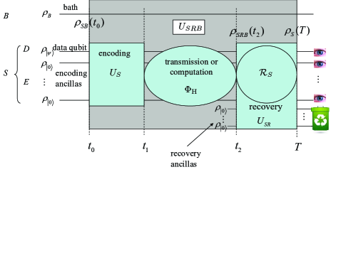
Figure 1: The initial system-bath state is the generically non-VQD state $\rho_{SB}(t_{0})$. The encoded system $S=D+E$ consists of data qubits $D$ and encoding ancillas $E$. We also include the recovery ancillas $R$, which are assumed to be completely isolated until they are brought into contact with $S$ and $B$ at a later time. Thus the full initial state is $\rho_{SB}(t_{0})\otimes\rho_{R}(t_{0})$. The overall evolution is governed by the unitary $U_{SRB}$ which acts on the system $S$, the bath $B$, and eventually the recovery ancillas $R$, and is denoted by the large grey box. The state of the data qubits is $\rho_{|\psi\rangle}=\mathrm{Tr}_{E,B}[\rho_{SB}(t_{0})]$, a state which is as close as possible (by isolating the system) to the desired pure data state $|\psi\rangle$. The state of each of the encoding ancillas is $\rho_{|0\rangle}=\mathrm{Tr}_{E^{\prime},B}[\rho_{SB}(t_{0})]$, a state which is as close as possible (again, by isolating the system) to the desired pure encoding ancilla state $|0\rangle$. Here $\mathrm{Tr}_{E,B}$ denotes a partial trace over all encoding ancillas and the bath, $\mathrm{Tr}_{E^{\prime},B}$ denotes a partial trace over all but one of the encoding ancillas, and the bath. Ideally, the encoding unitary $U_{S}$ is then applied to the encoded system. This is of course an idealization since in reality the encoding operation will not be a perfect unitary; instead what is really applied is $U_{SRB}(t_{1},t_{0})$, which is supposedly close to the ideal $U_{S}\otimes I_{R}\otimes I_{B}$. Thus, after the encoding the total state is $\rho_{SRB}(t_{1})=U_{SRB}(t_{1},t_{0})[\rho_{SB}(t_{0})\otimes\rho_{R}(t_{0})]U_{SRB}^{{\dagger}}(t_{1},t_{0})$ and the encoded system state is $\rho_{S}(t_{1})=\mathrm{Tr}_{R,B}[\rho_{SRB}(t_{1})]$. The system is then passed through the noise channel for the purpose of either computation or communication, i.e., $\rho_{SRB}(t_{2})=U_{SRB}(t_{2},t_{1})\rho_{SRB}(t_{1})U_{SRB}^{{\dagger}}(t_{2},t_{1})$, whence $\rho_{S}(t_{2})=\mathrm{Tr}_{R,B}[\rho_{SRB}(t_{2})]=\Phi_{\mathrm{H}}[\rho_{S}(t_{1})]$, where $\Phi_{\mathrm{H}}$ is a Hermitian noise map since $\rho_{SRB}(t_{1})$ is generically a non-VQD state due to the initial non-classical correlations between $S$ and $B$. The goal of the error correction procedure is to recover the original encoded system state from $\rho_{S}(t_{2})$, and to this end we introduce recovery ancillas $R$ at $t_{2}$. Similarly to the encoding ancillas, these recovery ancillas are each in the state $\rho_{|0\rangle}=\mathrm{Tr}_{S,R^{\prime},B}[\rho_{SRB}(t_{2})]$, a state which is as close as possible to the desired pure recovery ancilla state $|0\rangle$. Next, ideally the recovery unitary $U_{SR}\otimes I_{B}$ is applied. In reality what is applied is $U_{SRB}(T,t_{2})$, which is supposedly close to the ideal $U_{SR}\otimes I_{B}$. Then the recovery ancillas are discarded and possibly recycled, leaving the encoded system in the final state $\rho_{S}(T)=\mathrm{Tr}_{R,B}[\rho_{SRB}(T)]=\mathcal{R}_{S}[\rho_{S}(t_{2})]$, which can be measured. Since $\rho_{SRB}(t_{2})$ is generically not a VQD state (due to non-classical correlations between $S$ and $R$, mediated by their mutual interaction with $B$), it is clear that the recovery map $\mathcal{R}_{S}$ is generically a non-CP Hermitian map. We recover the CP recovery map scenario if, for example, $\rho_{SRB}(t_{2})=\rho_{SB}(t_{2})\otimes\rho_{R}(t_{2})$. The assumption that this is not the case is consistent with the working premise of this paper and is equivalent in that regard to the assumption that the initial system-bath state is not of the form $\rho_{SB}(t_{0})=\rho_{S}(t_{0})\otimes\rho_{B}(t_{0})$.

IV.3.3 How does non-CP, Hermitian recovery arise?

In standard QEC theory the recovery map is considered CP. The reason for this is that the recovery ancillas are introduced after the action of the noise channel so that they enter in a tensor product state with the encoded qubits that underwent the noise channel. The recovery map is obtained in the standard setting by first applying a unitary over the encoded qubits plus recovery ancillas, then tracing out the recovery ancillas. This is manifestly a CP map over the encoded qubits.

Since we know that the recovery map experienced by the encoded qubits is CP if and only if the initial state of the encoded and recovery ancilla qubits has vanishing quantum discord ShabaniLidar:08 , it is clear how a non-CP recovery map can be implemented: the recovery ancillas should have non-vanishing quantum discord with the encoded qubits. Since this will still be a QDP, the resulting recovery map will be Hermitian according to Theorem 3.

Such a situation can come about in various ways. For example, a scenario which is particularly relevant for quantum computation and communication, is one where the environment causes the recovery ancillas to become non-classically correlated with the encoded qubits before the recovery operation can be applied. This is a reasonable scenario since, while the recovery ancillas are presumably kept pure and isolated from the environment for as long as possible, at some point they must be brought into contact with the encoded qubits, and at this point all qubits (encoded and recovery ancillas) are susceptible to correlations mediated by the environment. This is shown in Fig. 1.

V Conclusions

This work aimed to fill two gaps: one in the theory of open quantum systems, and a resulting gap in the theory of quantum error correction. The first gap had to do with the type of maps that describe open systems given arbitrary initial states of the total system. In fact, it was not a priori clear that there should even be a linear map connecting the initial to the final open system state for arbitrary initial total system states. Building upon the class of “special linear states” we introduced in ShabaniLidar:08 we showed here that in fact such a linear map description does always exist, and moreover, for quantum dynamics the map is always Hermitian. The map reduces to the completely positive type if and only if the initial total system state has vanishing quantum discord ShabaniLidar:08 ; in all other cases it is Hermitian but not CP. This result, we argued, impacts the theory of quantum error correction, where previously the assumption of CP maps was taken for granted. In the second part of this work we filled this gap in QEC theory, by developing a theory of Linear Quantum Error Correction (LQEC), which generalizes the CP-map-based standard theory of QEC. We showed that to every linear map $\Phi_{\mathrm{L}}$ is associated a CP map which, if correctable, also provides an encoding with corresponding CP recovery map for $\Phi_{\mathrm{L}}$ (Theorem 4). Moreover, it is possible to find a non-CP recovery for $\Phi_{\mathrm{L}}$ within a larger class of codes (Theorem 5). From a physical standpoint this result is actually too general, since only Hermitian maps ever arise from quantum dynamics [to the extent that the standard quantum dynamical process (2) is valid]. Hence we specialized LQEC to the Hermitian maps case, and showed that in this case standard QEC theory for CP maps already suffices, in the sense that it is legitimate to replace a given Hermitian noise map by a corresponding CP map obtained simply by taking the absolute values of all the Hermitian map coefficients. Any QEC code which corrects this CP map will also correct the original Hermitian map (Corollary 1). Nevertheless, there is room for a genuine generalization when one considers Hermitian maps, since it is also possible to perform QEC using Hermitian recovery maps (Corollary 2). We argued that, in fact, recovery maps will generically be non-CP Hermitian maps, since recovery ancillas that are introduced into a quantum circuit prior to the recovery step will become non-classically correlated with the environment and consequently with the rest of the system.

An interesting open question for future studies is whether the results presented here have an impact on the threshold for fault tolerant quantum error correction. For example, note that while CP recovery perfectly returns the encoded state [Eqs. (29) and (41)], non-CP recovery only does so up to a proportionality factor which depends on the details of the noise and recovery maps [$F_{\mathrm{L}}$ in Eq. (32) and $F_{\mathrm{H}}$ in Eq. (43)]. This proportionality factor – assuming non-CP recovery is applied – may differ for different terms in the fault path decomposition Aharonov:08 , an effect which may propagate into the value of the fault tolerance threshold. This requires careful analysis, which is beyond the scope of this paper.

Appendix A Proof of Theorem 1

We use a method similar to Choi’s proof for a CP map representation Choi:75 , recently clearly reviewed in Ref. Leung:03 . The main difference between the proofs in Refs. Choi:75 ; Leung:03 and our proof is that in the previous proofs positivity allowed for the use of standard diagonalization, whereas in the absence of positivity we use the singular value decomposition Horn:book .

Proof. Eq. (4) immediately implies that $\Phi_{\mathrm{L}}$ is a linear map. For the other direction, let $\widetilde{M}=\sum_{i,j=1}^{n}|i\rangle\langle j|\otimes|i\rangle\langle j|=n|\phi\rangle\langle\phi|$, where $|i\rangle$ is a column vector with $1$ at position $i$ and $0$’s elsewhere, and $|\phi\rangle=n^{-1/2}\sum_{i}|i\rangle\otimes|i\rangle$ is a maximally entangled state over $\mathcal{H}\otimes\mathcal{H}$, where $\mathcal{H}$ is the Hilbert space spanned by $\{|i\rangle\}_{i=1}^{n}$. $\widetilde{M}$ is also an $n\times n$ array of $n\times n$ matrices, whose $(i,j)$th block is $|i\rangle\langle j|$. Construct two equivalent expressions for $(\mathcal{I}\otimes\Phi_{\mathrm{L}})[\widetilde{M}]$, where $\mathcal{I}$ is the $(n\times n)\times(n\times n)$ identity matrix. (i) $(\mathcal{I}\otimes\Phi_{\mathrm{L}})[\widetilde{M}]$ is an $n\times n$ array of $m\times m$ matrices, whose $(i,j)$th block is $\Phi_{\mathrm{L}}[|i\rangle\langle j|]$. (ii) Consider a singular value decomposition: $(\mathcal{I}\otimes\Phi)[\widetilde{M}]=UDV=\sum_{\alpha}\lambda_{\alpha}U|\alpha\rangle\langle\alpha|V=\sum_{\alpha}\lambda_{\alpha}|u_{\alpha}\rangle\langle v_{\alpha}|$. Here $U$ and $V$ are unitary, $D=\mathrm{diag}(\{\lambda_{\alpha}\})$ is diagonal and $\lambda_{\alpha}\geq 0$ are the singular values of $(\mathcal{I}\otimes\Phi_{\mathrm{L}})[\widetilde{M}]$. Divide the column (row) vector $|u_{\alpha}\rangle$ ($\langle v_{\alpha}|$) into $n$ segments each of length $m$ and define an $m\times n$ ($n\times m$) matrix $E_{\alpha}$ ($E_{\alpha}^{\prime}$) whose $i$th column (row) is the $i$th segment; then $E_{\alpha}|i\rangle$ ($\langle i|E_{\alpha}^{\prime\dagger}$) is the $i$th segment of $|u_{\alpha}\rangle$ ($\langle v_{\alpha}|$). Therefore the $(i,j)$th block of $|u_{\alpha}\rangle\langle v_{\alpha}|$ becomes $E_{\alpha}|i\rangle\langle j|E_{\alpha}^{\prime\dagger}$.

Equating the two expressions in (i) and (ii) for the $(i,j)$th block of $(\mathcal{I}\otimes\Phi_{\mathrm{L}})[\widetilde{M}]$, we find $\Phi_{\mathrm{L}}[|i\rangle\langle j|]={\sum_{\alpha}}\lambda_{\alpha}E_{\alpha}|i\rangle\langle j|E_{\alpha}^{\prime\dagger}$. Since $\lambda_{\alpha}\geq 0$ we can redefine $E_{\alpha}$ as $\sqrt{\lambda_{\alpha}}E_{\alpha}$ and $E_{\alpha}^{\prime}$ as $\sqrt{\lambda_{\alpha}}E_{\alpha}^{\prime}$, which we do from now on. Finally, the linearity assumption on $\Phi_{\mathrm{L}}$, together with the fact that the set $\{|i\rangle\langle j|\}_{i,j=1}^{n}$ spans $\mathfrak{M}_{n}$, implies Eq. (4).

Next let us prove Eq. (5) for Hermitian maps. For an old proof that uses very different techniques see Ref. Hill:73 . Eq. (5) immediately implies that $\Phi_{\mathrm{H}}$ is a Hermitian map. For the other direction, associate a matrix $L_{\Phi_{\mathrm{H}}}$ with the Hermitian map $\Phi_{\mathrm{H}}$: $\rho^{\prime}=\Phi_{\mathrm{H}}(\rho)$ $\Longleftrightarrow$ $\rho_{m\mu}^{\prime}=L_{n\nu}^{m\mu}\rho_{n\nu}$ (summation over repeated indices is implied). Hermiticity of $\rho$ and its image $\rho^{\prime}$ implies $\rho_{\mu m}^{\prime}=\rho_{m\mu}^{\prime\ast}=L_{n\nu}^{m\mu\ast}\rho_{n\nu}^{\ast}=L_{n\nu}^{m\mu\ast}\rho_{\nu n}$, i.e., $L_{n\nu}^{m\mu\ast}=L_{\nu n}^{\mu m}$ Zyczkowski:04 . We can use this property of $L_{\Phi_{\mathrm{H}}}$ to show that if $\Phi_{\mathrm{H}}$ is a Hermitian map, then $\mathcal{I}\otimes\Phi_{\mathrm{H}}$ is Hermiticity preserving. Consider $\mathcal{M}=\mathcal{M}_{k\xi}^{n\nu}|k\rangle\langle\xi|\otimes|n\rangle\langle\nu|$. Then $\mathcal{M}^{\prime}=(\mathcal{I}\otimes\Phi_{\mathrm{H}})[\mathcal{M}]=\mathcal{M}_{k\xi}^{n\nu}|k\rangle\langle\xi|\otimes\Phi_{\mathrm{H}}(|n\rangle\langle\nu|)=\mathcal{M}_{k\xi}^{m\mu}|k\rangle\langle\xi|\otimes L_{n\nu}^{m\mu}|n\rangle\langle\nu|$. Assume that $\mathcal{M}_{k\xi}^{m\mu\ast}=\mathcal{M}_{\xi k}^{\mu m}$. This property holds for $\mathcal{M}=\widetilde{M}=|\phi\rangle\langle\phi|$ where $|\phi\rangle=\dim(\mathcal{H})^{-1/2}\sum_{i}|i\rangle\otimes|i\rangle$ is a maximally entangled state over $\mathcal{H}\otimes\mathcal{H}$ ($\mathcal{M}_{\xi k}^{\mu m}\equiv 1$). Then $\mathcal{M}^{\prime{\dagger}}=\mathcal{M}_{k\xi}^{m\mu\ast}|\xi\rangle\langle k|\otimes L_{n\nu}^{m\mu\ast}|\nu\rangle\langle n|=\mathcal{M}_{\xi k}^{\mu m}|\xi\rangle\langle k|\otimes L_{\nu n}^{\mu m}|\nu\rangle\langle n|=\mathcal{M}^{\prime}$. Therefore $(\mathcal{I}\otimes\Phi_{\mathrm{H}})[|\phi\rangle\langle\phi|]$ is Hermitian, and in particular invertible. It follows that the SVD used in the proof of Theorem 1 can be replaced by standard diagonalization ($U=V^{{\dagger}}$). In this case the left and right singular vectors $|u_{\alpha}\rangle=\langle v_{\alpha}|^{{\dagger}}$ are the eigenvectors of $(\mathcal{I}\otimes\Phi_{\mathrm{H}})[|\phi\rangle\langle\phi|]$ and $c_{\alpha}=\lambda_{\alpha}$ are its eigenvalues. Then $E_{\alpha}=E_{\alpha}^{\prime}$ in Eq. (4) and $c_{\alpha}\in\mathbb{R}$.   

We note that by splitting the spectrum of $(\mathcal{I}\otimes\Phi_{\mathrm{H}})[|\phi\rangle\langle\phi|]$ into positive and negative eigenvalues, $\{c_{\alpha}^{+}\geq 0\}$ and $\{c_{\alpha}^{-}\leq 0\}$, we have as an immediate corollary a fact that was also noted in Jordan:04 : Any Hermitian map can be represented as the difference of two CP maps: $\Phi(\rho)$ $={\sum_{\alpha}}c_{\alpha}^{+}E_{\alpha}^{+}\rho E_{\alpha}^{+\dagger}-{\sum_{\alpha}}|c_{\alpha}^{-}|E_{\alpha}^{-}\rho E_{\alpha}^{-\dagger}$.

Appendix B Direct Proof of Corollary 1

Proof. The operation elements of $\tilde{\Phi}_{\mathrm{CP}}$ are $\{{F}_{i}=\sqrt{{|}c_{i}|}K_{i}\}_{i=1}^{N}$, whence $\tilde{\Phi}_{\mathrm{CP}}(\rho)={\sum_{i=1}^{N}}F_{i}\rho F_{i}^{\dagger}$. The standard quantum error conditions (19) for $\tilde{\Phi}_{\mathrm{CP}}$ is a set of conditions in terms of the $F_{i}$:

$$PF_{i}^{{\dagger}}F_{j}P=\beta_{ij}P,\quad i,j\in\{1,\ldots,N\}.$$ (34)

The existence of a projector $P$ which satisfies Eq. (34) is equivalent to the existence of a QEC code for $\tilde{\Phi}_{\mathrm{CP}}$. Assuming that a code $\mathcal{C}$ has been found (i.e., $P\mathcal{C}=\mathcal{C}$) for $\tilde{\Phi}_{\mathrm{CP}}$, we use this as a code for $\Phi_{\mathrm{H}}$ and show that the corresponding CP recovery map $\mathcal{R}_{\mathrm{CP}}$ is also a recovery map for $\Phi_{\mathrm{H}}$. Indeed, let $G_{j}\equiv\sum_{i=1}^{N}u_{ij}F_{i}$ be new operation elements for $\tilde{\Phi}_{\mathrm{CP}}$, i.e., $\tilde{\Phi}_{\mathrm{CP}}={\sum_{j=1}^{N}}G_{j}\rho G_{j}^{\dagger}$, where $u$ is the unitary matrix that diagonalizes the Hermitian matrix $\beta=[\beta_{ij}]$, i.e., $u^{{\dagger}}\beta u=d$. Let $\mathcal{R}_{\mathrm{CP}}=\{R_{k}\}$ be the CP recovery map for $\tilde{\Phi}_{\mathrm{CP}}$. Assume that $\rho$ is in the code space, i.e., $P\rho P=\rho$. We now show that $\mathcal{R}_{\mathrm{CP}}[\Phi_{\mathrm{H}}(\rho)]=\rho$, i.e., we have CP recovery. First,

$$\mathcal{R}_{\mathrm{CP}}[\Phi_{\mathrm{H}}(\rho)] = \sum_{k}R_{k}\left(\sum_{i=1}^{N}\frac{c_{i}}{|c_{i}|}F_{i}\rho F_{i}^{{\dagger}}\right)R_{k}^{{\dagger}}$$ (35)

$$= \sum_{i=1}^{N}\frac{c_{i}}{|c_{i}|}\sum_{j,j^{\prime}=1}^{N}u_{ij}^{\ast}u_{ij^{\prime}}$$

$$\times\sum_{k}\left(R_{k}G_{j}P\right)\rho\left(PG_{j^{\prime}}^{{\dagger}}R_{k}^{{\dagger}}\right).$$

Now, note that, using Eq. (34):

$$PG_{k}^{{\dagger}}G_{l}P = \sum_{ij}u_{ik}^{\ast}u_{jl}PF_{i}^{{\dagger}}F_{j}P=\sum_{ij}u_{ik}^{\ast}\beta_{ij}u_{jl}P$$ (36)

$$= d_{k}\delta_{kl}P.$$

Then the polar decomposition yields $G_{k}P=U_{k}(PG_{k}^{{\dagger}}G_{k}P)^{1/2}=\sqrt{d_{k}}U_{k}P$. The recovery operation elements are given by

$$R_{k}=U_{k}^{{\dagger}}P_{k};\quad P_{k}=U_{k}PU_{k}^{{\dagger}}.$$ (37)

Therefore $P_{k}=G_{k}PU_{k}^{{\dagger}}/\sqrt{d_{k}}$. This allows us to calculate the action of the $k$th recovery operator on the $l$th error:

$$R_{k}G_{l}P = U_{k}^{{\dagger}}P_{k}^{{\dagger}}G_{l}P=U_{k}^{{\dagger}}(U_{k}PG_{k}^{{\dagger}}/\sqrt{d_{k}})G_{l}P$$ (38)

$$= \delta_{kl}\sqrt{d_{k}}P.$$

Therefore,

$$\mathcal{R}_{\mathrm{CP}}[\Phi_{\mathrm{H}}(\rho)] = \sum_{i=1}^{N}\frac{c_{i}}{|c_{i}|}\sum_{j,j^{\prime}=1}^{N}u_{ij}^{\ast}u_{ij^{\prime}}$$ (39)

$$\times\sum_{k}\left(\delta_{kj}\sqrt{d_{k}}P\right)\rho\left(P\sqrt{d_{k}}\delta_{kj^{\prime}}\right)$$

$$= \rho\sum_{i=1}^{N}\frac{c_{i}}{|c_{i}|}\left(udu^{{\dagger}}\right)_{ii}$$

$$= (\sum_{i=1}^{N}\frac{c_{i}}{|c_{i}|}\beta_{ii})\rho.$$

Next note that, using condition (34) and trace preservation by $\Phi_{\mathrm{H}}$:

$$PF_{i}^{{\dagger}}F_{i}P = \beta_{ii}P\Longrightarrow\sum_{i=1}^{N}\frac{c_{i}}{|c_{i}|}\beta_{ii}P$$ (40)

$$= P\sum_{i=1}^{N}\frac{c_{i}}{|c_{i}|}F_{i}^{{\dagger}}F_{i}P=P\sum_{i=1}^{N}c_{i}K_{i}^{{\dagger}}K_{i}P=P$$

$$\Longrightarrow \sum_{i=1}^{N}\frac{c_{i}}{|c_{i}|}\beta_{ii}=1.$$

Hence, finally:

$$\mathcal{R}_{\mathrm{CP}}[\Phi_{\mathrm{L}}(\rho)]=\rho$$ (41)

for any $\rho$ in the codespace.   

Appendix C Proof of Corollary 2

Proof. Let $\{{F}_{i}=\sqrt{{|}c_{i}|}K_{i}\}_{i=1}^{N}$; we simply use the identities given in the proof of the previous theorem – specifically Eq. (39) – to calculate $\mathcal{R}_{\mathrm{H}}\circ\Phi_{\mathrm{H}}(\rho)$

$$\mathcal{R}_{\mathrm{H}}[\Phi_{\mathrm{H}}(\rho)] = \sum_{k}h_{k}R_{k}\left(\sum_{i=1}^{N}\frac{c_{i}}{|c_{i}|}F_{i}\rho F_{i}^{{\dagger}}\right)R_{k}^{{\dagger}}$$ (42)

$$= \sum_{i=1}^{N}h_{k}\frac{c_{i}}{|c_{i}|}\sum_{j,j^{\prime}=1}^{N}u_{ij}^{\ast}u_{ij^{\prime}}\times$$

$$\sum_{k}\left(\delta_{kj}\sqrt{d_{k}}P\right)\rho\left(P\sqrt{d_{k}}\delta_{kj^{\prime}}\right)$$

$$= P\rho P\sum_{i=1}^{N}\frac{c_{i}}{|c_{i}|}\sum_{k}h_{k}u_{ik}^{\ast}u_{ik}d_{k}$$

$$= F_{\mathrm{H}}P\rho P\propto\rho,$$

where

$$F_{\mathrm{H}}\equiv\sum_{i=1}^{N}\frac{c_{i}}{|c_{i}|}\left(udhu^{{\dagger}}\right)_{ii},$$ (43)

where $h\equiv\mathrm{diag}(\{h_{k}\})$, and $F_{\mathrm{H}}$ is a “correction factor” for Hermitian recovery of Hermitian noise maps, which was $1$ in the case of CP recovery, above.

References

• (1) E.B. Davies, Quantum Theory of Open Systems (Academic Press, London, 1976).
• (2) R. Alicki and K. Lendi, Quantum Dynamical Semigroups and Applications, No. 286 in Lecture Notes in Physics (Springer-Verlag, Berlin, 1987).
• (3) H.-P. Breuer and F. Petruccione, The Theory of Open Quantum Systems (Oxford University Press, Oxford, 2002).
• (4) M.A. Nielsen and I.L. Chuang, Quantum Computation and Quantum Information (Cambridge University Press, Cambridge, UK, 2000).
• (5) F. Gaitan, Quantum Error Correction and Fault Tolerant Quantum Computing (CRC Press, Boca Raton, 2008).
• (6) K. Kraus, States, Effects and Operations, Fundamental Notions of Quantum Theory (Academic, Berlin, 1983).
• (7) E. Knill and R. Laflamme, Phys. Rev. A 55, 900 (1997).
• (8) R. Alicki, Phys. Rev. Lett. 75, 3020 (1995), Comment on “Reduced Dynamics Need Not Be Completely Positive”; Reply by P. Pechukas, ibid., p. 3021.
• (9) P. Stelmachovic and V. Buzek, Phys. Rev. A 64, 062106 (2001).
• (10) T.F. Jordan, A. Shaji, and E.C.G. Sudarshan, Phys. Rev. A 70, 052110 (2004).
• (11) H. A. Carteret, D. R. Terno, and K. Życzkowski, Phys. Rev. A 77, 042113 (2008).
• (12) C.A. Rodríguez, K. Modi, A.-M. Kuah, E.C.G. Sudarshan, A. Shaji, J. Phys. A 41, 205301 (2008).
• (13) A. Shabani and D. A. Lidar, eprint arXiv.org:0808.0175 (in press, Phys. Rev. Lett.).
• (14) H. Ollivier and W.H. Zurek, Phys. Rev. Lett. 88, 017901 (2001).
• (15) R. Alicki, D. A. Lidar, and P. Zanardi, Phys. Rev. A 73, 052311 (2006).
• (16) D. M. Tong, L. C. Kwek, C. H. Oh, J.-L. Chen, and L. Ma, Phys. Rev. A 69, 054102 (2004).
• (17) W. F. Stinespring, Proc. Am. Math. Soc. 6, 211 (1955).
• (18) L. Jakóbczyk and M. Siennicki, Phys. Lett. A 286, 383 (2001).
• (19) G. Kimura, Phys. Lett. A 314, 339 (2003).
• (20) M.S. Byrd and N. Khaneja, Phys. Rev. A 68, 062322 (2003).
• (21) G. Kimura and A. Kossakowski, Open Sys. and Information Dyn. 12, 207 (2005).
• (22) P.W. Shor, in Proceedings of the 37th Symposium on Foundations of Computing (IEEE Computer Society Press, Los Alamitos, CA, 1996), p. 56.
• (23) D. Aharonov and M. Ben-Or, in Proceedings of 29th Annual ACM Symposium on Theory of Computing (STOC) (ACM, New York, NY, 1997), p. 46.
• (24) E. Knill, R. Laflamme and W. Zurek, Science 279, 342 (1998).
• (25) A.M. Steane, Phys. Rev. A 68, 042322 (2003).
• (26) E. Knill, Nature 434, 39 (2005).
• (27) B.W. Reichardt, in Automata, Languages and Programming, Vol. 4051 of Lecture Notes in Computer Science, edited by M. Bugliesi et al. (Springer, Berlin, 2006), Chap. 6, p. 50.
• (28) D. Aharonov and M. Ben-Or, SIAM J. Comput. 38, 1207 (2008).
• (29) P. Aliferis and J. Preskill, Phys. Rev. A 79, 012332 (2009).
• (30) B.M. Terhal, G. Burkard, Phys. Rev. A 71, 012336 (2005).
• (31) P. Aliferis, D. Gottesman, and J. Preskill, Quantum Inf. Comput. 6, 97 (2006).
• (32) D. Aharonov, A. Kitaev, J. Preskill, Phys. Rev. Lett. 96, 050504 (2006).
• (33) M.A. Nielsen, C.M. Caves, B. Schumacher and H. Barnum, Proc. Roy. Soc. London Ser. A 454, 277 (1998).
• (34) M.D. Choi, Linear Algebr. Appl. 10, 285 (1975).
• (35) D.W. Leung, J. Math. Phys. 44, 528 (2003).
• (36) R.A. Horn and C.R. Johnson, Matrix Analysis (Cambridge University Press, Cambride, UK, 1999).
• (37) R.D. Hill, Linear Algebra and its Applications 6, 257 (1973).
• (38) K. Zyczkowski and I. Bengtsson, Open Sys. & Information Dyn. 11, 342 (2004).