Localized magnetic states in Rashba dots

Abstract

We study the formation of local moments in quantum dots arising in quasi-one dimensional electron wires due to localized spin-orbit (Rashba) interaction. Using an Anderson-like model to describe the occurrence of the magnetic moments in these Rashba dots, we calculate the local magnetization within the mean-field approximation. We find that the magnetization becomes a nontrivial function of the Rashba coupling strength. We discuss both the equilibrium and nonequilibrium cases. Interestingly, we obtain a magnetic phase which is stable at large bias due to the Rashba interaction.

I Introduction

Spin-related phenomena have recently attracted much attention, as they are the key ingredient in the new field known as spintronics spintronic . Two-dimensional (2D) semiconductors are appropriate materials to be used in spintronics applications since they offer the possibility of an electric control of spins via tunable spin-orbit (SO) interaction. An important contribution to SO effects in 2D electronic states of narrow gap semiconductors (e.g, InAs) is the Rashba interaction ra . This interaction is a generalization of the vacuum SO interaction from the Pauli equation, $H_{so}=(e\hbar^{2}/4m^{2}c^{2}){\mathbf{\sigma}}\cdot(\mathbf{\nabla}V(r)\times\mathbf{k})$, which is small for non-relativistic momenta $\hbar k\ll mc$, $V(r)$ being the scalar potential. In semiconductors, the energy gap $E_{g}$ and the band splitting $\Delta$ are comparable in magnitude ($E_{g}\sim\Delta\sim 1eV$) and, as a consequence, the SO coupling is enhanced by a factor $m^{2}c^{2}/E_{g}$.

The Rashba interaction is a type of SO interaction arising when a 2D electron gas forms at the interface of a heterostructure. To lowest order in momentum, the Rashba Hamiltonian reads

$$H_{R}=\frac{1}{2\hbar}([\alpha,p_{y}]_{+}\sigma_{x}-[\alpha,p_{x}]_{+}\sigma_{y})\,,$$ (1)

where $\alpha$ is the Rashba coupling proportional to the electric field producing the confinement. We take the confinement direction along z. In Eq. (1), $\mathbf{p}=(p_{x},p_{y})$ is the 2D momentum and $\sigma_{i}(i=x,y,z)$ are the Pauli matrices.

We note that available experimental data ta on few-electron quantum dots have been discussed in terms of Rashba spin-orbit coupling and exchange interaction ko . Using the Spin Density Functional Theory it was showed go that the competition of this coupling and the exchange interaction gives rise to the suppression of the Hund rule, and a dot with a closed configuration presents a paramagnetic behavior. We have to mention that these result have been obtained in the absence of the Coulomb interaction.

When the Rashba interaction is localized around a finite region of a quasi one-dimensional ballistic wire [see Fig. 1(a)], Ref. sa1, predicts the formation of quasi-bound states which are coupled to the nonresonant background channel. Both the potential well and the intersubband coupling is produced by the Rashba interaction alone. Furthermore, the quasi-bound states lead to enhanced backscattering, causing strong dips in the conductance curves of the wire as a function of the Fermi energy.zhang Since both the level position and broadening can be tuned with the Rashba strength $\alpha$, these states are termed Rashba dots sa1 .

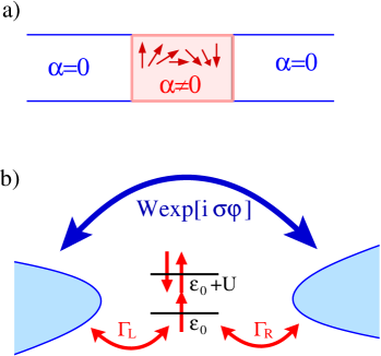
Figure 1: (Color online). (a) The system under study consists of a quantum wire with a region of localized spin-orbit interaction of the Rashba type ($\alpha$ is the Rashba coupling strength). Interactions are restricted to the Rashba dot. (b) Mapping of the upper system onto a quasi-localized level and a nonresonant background channel with spin dependent couplings to external leads.

Recently, López et al. lo have formulated a microscopic theory for transport across Rashba dots including Coulomb interactions in the dot. An important aspect of this model is that different regimes can be achieved by tuning the parameters of the Rashba Hamiltonian and this can be done modulating external electric fields applied to nearby gates. The difference between the Anderson Hamiltonian and and the Hamiltonian proposed in Ref. lo, is twofold. First, in the Anderson Hamiltonian the spin is conserved at low temperatures, leading to the Kondo effect, but in Ref. lo, the Rashba dot Hamiltonian contains a spin-flip interaction because the localized states couple to the continuum states with opposite spins. Second, due to the Rashba induced precession term, the direct transmission channel presents a phase term similar to the Aharonov-Bohm case, but the phase is now spin-dependent ac . Remarkably, despite these differences the system shows a persisting Kondo effect at low temperatures but with a novel gate dependence lo .

In this paper, we address the magnetic properties of Rashba dots. We follow Anderson’s model for magnetic impurities in a metallic host and determine whether it is energetically favorable for the dot to form a localized magnetic moment. We show below that the Coulomb interaction can develop magnetic moments in a Rashba dot for a critical value of the ratio $(U/\Gamma)_{\rm crit}$, which depends of the parameters of the Rashba interaction. Our results might also be important for quantum dots doped with magnetic impurities le ; fe . Magnetic ordering in dots can be induced by the Coulomb interaction and the magnetization can be electrically controlled even for a fixed number of electrons zu1 ; zu2 .

This paper is organized as follows. We present in section II the model and calculate the Green function using the equation of motion method. The magnetic moment is determined in section III both for the equilibrium and the nonequilibrium cases. The main results are compared with exact numerical calculations in Sec. IV. The results are discussed in section V, which also contains our conclusions.

II Theoretical Model

We start with the model Hamiltonian:

$$H=H_{e}+H_{d}+H_{W}+H_{V}\,,$$ (2)

where

$$H_{e} = \sum_{\alpha,k,\sigma}\epsilon_{\alpha,k,\sigma}c_{\alpha,k,\sigma}^{{\dagger}}c_{\alpha,k,\sigma}\,,$$

$$H_{d} = \sum_{\sigma}\epsilon_{d}d_{\sigma}^{{\dagger}}d_{\sigma}+Un_{\sigma}n_{-\sigma}\,,$$

$$H_{W} = \sum_{k,\sigma}(We^{is_{\sigma}\varphi}c_{L,k,\sigma}^{{\dagger}}c_{R,k,\sigma}+H.c.)\,,$$

$$H_{V} = \sum_{\alpha,k,\sigma}(Vc_{\alpha,k,\sigma}^{{\dagger}}d_{-\sigma}+H.c.)\,.$$ (3)

In this Hamiltonian we consider the spin quantization axis along the Rashba field (the $y$ direction for transport along $x$), $n_{\sigma}=d_{\sigma}^{{\dagger}}d_{\sigma}$ is the occupation number for electrons in the Rashba dot with spin $\sigma=\uparrow,\downarrow$ and $c_{\alpha,k,\sigma}^{{\dagger}}$ is the creation operator of continuum electrons with wave vector $k$ and spin $\sigma$ in the lead $\alpha=L,R$. The nonresonant channel is described with the term $H_{W}$ where the propagation phase acquired by a transmitted electron is spin-dependent ($s_{\sigma}=\pm 1$ if $\sigma=\uparrow,\downarrow$). Finally, localized and extended electronic states are coupled via the interaction $H_{V}$. A pictorial representation of $H$ is shown in Fig. 1(b).

The parameters of this Hamiltonian are $U=U(\alpha,l)$, $V=V(\alpha,l)$ and $W=W(\alpha,l)$, where $l$ is the length of the Rashba induced square-well potential (we assume, for simplicity, that $\alpha(x)$ is constant if $0<x<l$ and zero otherwise) sa1 , and $\varphi=k_{R}l$ with $k_{R}=m\alpha/\hbar^{2}$. Importantly, these parameters can be externally controlled with gates by changing $\alpha$ and $l$.

The form of $H$ is similar to the Hamiltonian describing the transport in a device formed by an Aharonov-Bohm interferometer with a quantum dot in one of its arms ho but they differ in that the phases in the interaction term $W$ depend on the spin direction, and that each hopping process through the dot is associated with a spin-flip event. In the conventional Anderson model, spin is conserved, and this leads to Kondo correlations.

In order to study the occurrence of magnetic moments in this model we will calculate the Green function $G_{d\sigma}(\omega)\equiv\langle\langle d_{\sigma}|d_{\sigma}^{{\dagger}}\rangle\rangle$, which obeys the equation,

$$\omega G_{d\sigma}(\omega)=1+\langle\langle[d_{\sigma},H]|d_{\sigma}^{{\dagger}}\rangle\rangle\,.$$ (4)

In the mean-field approximation, the spin-dependent energy of the $d$-electrons is $\epsilon_{d,\sigma}=\epsilon_{d}+U\langle n_{-\sigma}\rangle$. Using the general equation-of-motion method, we find

$$[G_{d\sigma}(\omega)]^{-1} = \omega-\epsilon_{d\sigma}+\frac{1}{\Sigma}\sum_{\alpha k}\frac{2V^{2}}{\omega-\epsilon_{k}}$$ (5)

$$+ \frac{4W\cos\varphi}{\Sigma}\left(\sum_{k}\frac{V}{\omega-\epsilon_{k}}\right)^{2}\,,$$

where $\Sigma$ is given by the expression

$$\Sigma=1-\left(\sum_{k}\frac{W}{\omega-\epsilon_{k}}\right)^{2}$$ (6)

If we perform the summations over $k$ in the relations above, the Green function becomes

$$G_{d\sigma}(\omega)=\left[\omega-\epsilon_{d\sigma}+i\Gamma+\Gamma\sqrt{x}\cos\varphi\right]^{-1}\,,$$ (7)

where $\Gamma=\Delta/(1+x)$, $x=\pi^{2}W^{2}\nu^{2}$, $\Delta=\pi V^{2}\nu$, $\nu$ being the continuum density of states at the Fermi level $E_{F}$ (we take $\nu$ as a constant function of energy). We note that the tunneling broadening $\Delta$ becomes renormalized into $\Delta/(1+x)$ due to the background channel when $W\neq 0$. Furthermore, the spin contribution due to the Rashba interaction is proportional to $\cos\varphi$ for the both spin orientations.

III Magnetic moment

III.1 Equilibrium case

The magnetization along the Rashba field direction is given by the difference between the occupancy expectation value for spin up and spin down,

$$m=\langle n_{d\uparrow}\rangle-\langle n_{d\downarrow}\rangle\,.$$ (8)

At zero temperature, the occupation reads,

$$\langle n_{d\sigma}\rangle=\int_{-\infty}^{E_{F}}\rho_{d}(\omega)\,d\omega\,,$$ (9)

where $\rho_{d\sigma}(\omega)$ is the local density of states at the Rashba dot, defined in terms of the Green function as $\rho_{d\sigma}(\omega)=-\operatorname{Im}G_{d\sigma}(\omega)/\pi$.

Consider first the simple case $U=0$. Then,

$$\rho_{d\sigma}(\omega)=\frac{\Gamma}{\pi(\Gamma^{2}+\xi(\omega)^{2})}\,,$$ (10)

where $\xi$ is given by

$$\xi(\omega)=\omega-\epsilon_{d}+\Gamma\sqrt{x}\cos\varphi\,.$$ (11)

Since $U=0$, the energy $\xi$ is spin independent. Inserting Eq. (10) in Eq. (9), we obtain

$$\langle n_{d\sigma}\rangle=\frac{1}{2}-\frac{1}{\pi}\tan^{-1}\frac{\epsilon_{d}-E_{F}-\Gamma\sqrt{x}\cos\varphi}{\Gamma}\,.$$ (12)

Because $\langle n_{d\uparrow}\rangle=\langle n_{d\downarrow}\rangle$ even in the presence of spin-orbit interaction, we trivially have $m=0$. As expected, equilibrium magnetic states arise due to the presence of Coulomb interactions only.

Consider now the interacting case $U\neq 0$. We calculate the density of states using the spin dependence introduced by $\epsilon_{d\sigma}$ and we get:

$$\rho_{d\sigma}(\omega)=\frac{\Gamma}{\pi}\frac{1}{\xi_{-\sigma}(\omega)^{2}+\Gamma^{2}}\,,$$ (13)

where

$$\xi_{-\sigma}(\omega)=\omega-\epsilon_{d}+\Gamma\sqrt{x}\cos\varphi-U\langle n_{-\sigma}\rangle\,.$$ (14)

The occupation reads,

$$\langle n_{d\sigma}\rangle=\frac{1}{2}-\frac{1}{\pi}\tan^{-1}\frac{\epsilon_{d}-E_{F}+U\langle n_{d,-\sigma}\rangle-\Gamma\sqrt{x}\cos\varphi}{\Gamma}\,.$$ (15)

We analyze the formation of a magnetic state from the condition

$$\frac{d\langle n_{d\sigma}\rangle}{d\langle n_{d,-\sigma}\rangle}=-U\rho_{d,\sigma}(E_{F})\,.$$ (16)

As a consequence, the condition for the magnetic state that $d\langle n_{d}^{\sigma}\rangle/d\langle n_{d}^{-\sigma}\rangle<-1$ becomes

$$U\rho_{d}^{\sigma}(E_{F})>1\,.$$ (17)

This relation is similar to the Stoner condition for the occurrence of the magnetic state in the itinerant-electron systems, and the correlations effects appear only as an energy shift. A more accurate discussion, taking the energy dependence of $\Delta$ (via the density of states $\nu$) changes the magnetic region, which is known for a constant density of states. However, for our qualitative discussion we follow the wide-band approximation with a constant $\Delta$.

From Eqs. (8) and (15) we find a pair of self-consistent equations for the magnetization $m$ and the total electron density $n_{d}=\langle n_{d\uparrow}\rangle+\langle n_{d\downarrow}\rangle$:

$$m = \frac{1}{\pi}\sum_{\sigma}s_{\sigma}\cot^{-1}\frac{\frac{U}{2}(n_{d}-s_{\sigma}m)-\xi(E_{F})}{\Gamma}\,,$$ (18)

$$n_{d} = \frac{1}{\pi}\sum_{\sigma}\cot^{-1}\frac{\frac{U}{2}(n_{d}-s_{\sigma}m)-\xi(E_{F})}{\Gamma}\,,$$ (19)

From these two equations we calculate the size of the interaction above which a local moment develops. On the critical boundary describing the transition into the magnetic state, we approximately have $m\approx 0$ and $\langle n_{d\uparrow}\rangle\approx\langle n_{d\downarrow}\rangle\approx n_{d}$. Thus, we find

$$\left(\frac{U}{\Delta}\right)_{\rm crit}=\frac{\pi\ (1+c^{2})}{1+x}\,,$$ (20)

where $c=\cot{(\pi n_{d}/2)}$. This condition provides a number of interesting predictions. First, for increasing $x$ the function $(U/\Delta)_{\rm crit}$ decreases. Thus, the formation of magnetic moments is enhanced by the coupling to the continuum states, which is governed by the intensity of the Rashba interaction. Despite the fact that spin-orbit interactions are time-reversal symmetric and do not induce spontaneous magnetizations, indirectly the Rashba coupling makes it more favorable to generate magnetic solutions as compared to the case without Rashba interaction. If $x=0$ (or, equivalently, $W=0$) we recover the condition for the occurrence of the Anderson moments and . Second, $(U/\Delta)_{\rm crit}$ is a weakly function of the phase $\varphi$ since in Eq. (20) the dependence on $\varphi$ is only implicit through the total density $n_{d}$. Nevertheless, in the general case the condition given by Eq. (20) is far from being trivial since we recall that $U$, $\Delta$ and $n_{d}$ are complicated functions of the Rashba strength and the dot size lo .

III.2 Nonequilibrium case

We now turn to the nonequilibrium case, where a finite dc bias $V$ is applied between the two electrodes. The formation of magnetic moments within the Anderson Hamiltonian out of equilibrium has been recently analyzed by Komnik and Gogolin, see Ref. kom, . They find that the magnetic phase is stable at arbitrarily large voltages in the case of asymmetric couplings. Here, we assume symmetric couplings ($\Gamma_{L}=\Gamma_{R}$) and show below that even in this case the combination of Rashba interaction and finite bias leads to magnetic moment formation.

At nonequilibrium, the spin-dependent occupations are given by the Keldysh (lesser) Green function $G_{\sigma}^{<}(t,t^{\prime})=i\langle d_{\sigma}^{\dagger}(t)d_{\sigma}(t^{\prime})\rangle$,

$$\langle n_{\sigma}\rangle=\int_{-\infty}^{\infty}\frac{d\omega}{2\pi}\,{\rm Im}\,G_{\sigma}^{<}(\omega)$$ (21)

where $G_{\sigma}^{<}(\omega)$ is the Fourier transformed lesser Green function. We find

$$G_{\sigma}^{<}(\omega)=2i\Gamma\frac{\sqrt{x}\sin(s_{\bar{\sigma}}\varphi)(f_{L}-f_{R})/(1+x)+(f_{L}+f_{R})/2}{\xi(\omega)^{2}+\Gamma^{2}}\,,$$ (22)

where $f_{\alpha}=1/[1+e^{\beta(\omega-\mu_{\alpha})}]$ is the Fermi distribution function at the lead $\alpha=L,R$ with inverse temperature $\beta=1/k_{B}T$. Interestingly enough, the occupation depends on a term proportional to $\sin{(\bar{\sigma}\varphi)}$ which has a different sign for opposite spins. This term appears only at nonequilibrium ($f_{L}\neq f_{R}$). Therefore, we expect a spin polarization ($m\neq 0$) for a noninteracting Rashba dot ($U=0$) induced by the interplay effect of external bias and Rashba interaction.sun

We take $\mu_{L}=E_{F}+eV/2$ and $\mu_{R}=E_{F}-eV/2$ for the electrochemical potentials in the left and right contacts. As a result, we obtain a closed expression for the magnetization,

$$\begin{split}m&=-\frac{\sqrt{T_{r}}}{\pi}\sin\varphi\left[\tan^{-1}\frac{eV-2\xi(E_{F})}{2\Gamma}\right.\\ &\quad\left.+\tan^{-1}\frac{eV+2\xi(E_{F})}{2\Gamma}\right]\end{split}$$ (23)

where $T_{r}=4x/(1+x)^{2}$ is the background channel transmission. We infer that the magnetization is negative for positive $V$, arising from the orientation of the effective Rashba field, which points along $-y$ ser08 ; brus . The magnetization can be reversed if $\varphi$ changes sign (equivalently, the Rashba intensity $\alpha$). Obviously, the periodic dependence in Eq. (23) arises from the model but it is reasonable to assume a small $\alpha$. Therefore, $\varphi$ should not be very large. The periodic dependence on $\varphi$ is obtained in analogy with the Aharonov-Bohm effect and can be found in related spin-orbit systems (see, e.g., Ref. sun, ).

For $\varphi=\pi/2$ the minimum magnetization reads,

$$m_{\rm min}=-2\frac{\sqrt{T_{r}}}{\pi}\arctan\frac{eV}{2\Gamma}$$ (24)

which approaches $-1$ in the limits of $T_{r}\to 1$ and $eV\gg 2\Gamma$. On the other hand, for gate voltages much larger than the applied bias the magnetization approaches zero as

$$m=-\frac{\sqrt{T_{r}}}{\pi}\frac{\Gamma eV}{\varepsilon_{d}^{2}+\Gamma^{2}}$$ (25)

Finally, we note that the magnetization becomes finite and independent of the gate voltage in the limit of infinite $V$, in which case we find the simple expression $m=-\sqrt{T_{r}}$.

In the interacting case, one must replace $\xi(\omega)$ with $\xi_{-\sigma}(\omega)$ in Eq. (22). Then, the expression become involved and the full phase diagram can be obtained only numerically. However, the model is tractable in special cases. In particular, we focus on level energies around the particle-hole symmetric point ($\varepsilon_{d}=-U/2$). We define the dimensionless parameters $p=-\varepsilon_{d}/U$, $y=U/\Gamma$, $z=eV/2\Gamma$ and $R=2(\Gamma/U)\sqrt{x}\cos\varphi$. Our goal is to characterize the critical line that separates the nonmagnetic and the magnetic phases. This is given by a curve $p_{c}$ versus $y_{c}$ in the $p$–$y$ plane for different values of $z$. Then, for small values of $p_{c}-1/2$ we find (see the Appendix),

$$y_{c}\approx\frac{\pi}{2}(1+z^{2})\left[1+(1-3z^{2})\left[\frac{\pi}{2}(p_{c}-\frac{1}{2})+\frac{R_{o}}{1+z^{2}}\right]^{2}\right]\,,$$ (26)

where $R_{0}=\sqrt{x}\cos\varphi$. This result shows that the phase diagram presents a dip for $z>z^{\ast}$, where $z^{\ast}=1/\sqrt{3}$ (as in Ref. kom, ) but the form of the phase diagram is modified by the Rashba parameter $R$. In fact, the dip position shifts away from the symmetric point due to the Rashba induced level renormalization. The most important consequence is that whereas $m$ vanishes for $\varepsilon_{d}=-U/2$ at large bias in the case without spin-orbit interactions kom , the magnetization remains finite in the Rashba case. We have numerically checked this prediction (see below).

Figure 2: (Color online). Equilibrium magnetization of the Rashba dot for $\Delta=0.2$ and the values of $x$ and $\varphi$ shown in the figure.

IV Numerical results

IV.1 Equilibrium case

We now numerically solve Eqs. (8) and (15). For simplicity, we neglect the dependence of the system parameters on $\alpha$ and treat $U$, $\Delta$ and $\varepsilon_{d}$ as independent constants. In Fig. 2 we show $m$ as a function of $\varepsilon_{d}$ for $E_{F}=0$ and a fixed value of $\Delta$. In the absence of spin-orbit interaction ($x=0$ and $\varphi=0$) the magnetization is zero for positive $\varepsilon_{d}/U$. When $\varepsilon_{d}/U$ decreases, there is a transition point into the magnetic state, whose magnetization becomes maximal at the particle-hole symmetric point ($\varepsilon_{d}=-U/2$). At this point, $m\approx 0.64$, in agreement with Ref. and, . We now change the value of $x$ and $\varphi$. These two parameters can be modified independently tuning $\alpha$ and $l$. Then, for nonzero $x$ and $\varphi=0$ we find that the transition point shifts toward larger values of $\varepsilon_{d}/U$. This results from the self-energy shift $\Gamma\sqrt{x}\cos\varphi$ found in Eq. (7). Moreover, we observe an increase in the amplitude of $m$ as $x$ increases. This is a consequence of the Rashba coupling enhanced magnetic moment formation discussed above [Eq. (20)]. Furthermore, keeping $x$ constant and changing $\varphi$ we find that the magnetization curve changes only slightly, confirming our earlier prediction.

Figure 3: (Color online). Nonequilibrium magnetization of the Rashba dot for $\Delta=0.2$, $x=0.1$, $\varphi=\pi/2$ as a function of the level position for different values of the bias voltage $V$ in the noninteracting case ($U=0$).

IV.2 Nonequilibrium case

The nonequilibrium magnetization for the noninteracting case ($U=0$) is shown in Fig. 3 for increasing values of the external bias $V$. The curves are symmetric around $\varepsilon_{d}=0$, which corresponds to the alignment between $\varepsilon_{d}$ and the Fermi energy. The magnetization is nonzero for all finite values of $V$, as discussed after Eq. (22). In the limit of large voltages, the curve becomes featureless according to Eq. (24).

The interacting case is shown in Fig. 4. All energies are given in units of $U=1$. For comparison, we also reproduce the curve corresponding to $U=0$ and $eV=0.1$. At the same voltage in the interacting case, we observe that the magnetization curve follows the noninteracting curve for large $\varepsilon_{d}$. This is reasonable since we are entering the empty orbital regime for which interactions are unimportant. In the opposite regime, i.e., for negative $\varepsilon_{d}$, strong correlations start to dominate and the interacting magnetization, although still finite, departs significantly from the noninteracting case. We obtain strong modifications in the magnetization curve for increasing voltages, favoring the development of magnetic moments due to the combined influence of interactions and spin-orbit coupling. For energies around the particle-hole symmetric point ($\varepsilon_{d}\approx-U/2$), we find that the magnetization is reduced as $V$ increases but, unlike the case without spin-orbit interactions, $m$ does not vanish in the limit of large bias. This is excellent agreement with the prediction of Eq. (26).

Figure 4: (Color online). Nonequilibrium magnetization of the Rashba dot for $\Delta=0.2$, $x=0.1$, $\varphi=\pi/2$ as a function of the level position for different values of the bias voltage $V$ in the interacting case ($U=1$).

V Conclusions

We have studied the possibility of the occurrence of the magnetic models in a Rashba dot. The mean-field approximation has been used to calculate the magnetic moment and the critical value $U/\Delta$ for the occurrence of the local moments as function of the parameters of the Rashba Hamiltonian. This condition, expressed by Eq. (20), is similar to the condition obtained for the Anderson model,and but contains also the parameter $x$ which is determined by the Rashba interaction. Therefore, our calculation suggests a driving of magnetic moments by external electric fields via the Rashba interaction. We have demonstrated that the value of the local magnetization $m$ at equilibrium depends on $x$, but it is worth noting that the curve $m(\epsilon_{d}/U)$ is not very sensitive to the change of the parameter $\varphi$. This result has been also shown in numerical simulations of the mean-field equations.

As in the standard Anderson calculation,and our mean-field approach breaks the local symmetry but in an exact solution accounting also for the effect of the spin fluctuations we should recover the spin rotational invariance. Nevertheless, even if the magnetic states found above are an artefact of the model, the mean field solution is interesting as such since it gives an indication of the region of the coupling constants of the Hamiltonian where the fluctuations give a relevant effect. Recently, magnetic moment formation was proposed as a mechanism to explain the temperature dependence of the conductance for different gate voltages in quantum point contacts,me ; co where the scaling behavior of the conductance close to pinch-off as a function of temperature was used as an argument for the Kondo effect occurrence. Hence, our results can be useful for these systems when spin-orbit interactions become relevant. We believe that our calculation can also be important for magnetic semiconductors.le ; ichi .

In the nonequilibrium regime, we have discussed the interplay between an external bias and the on-site interaction energy when the spin-orbit interaction is present. The phase diagram we obtain is different from the nonequilibrium case studied in Ref. kom, , where the spin-orbit coupling was not considered. In Ref. kom, , it is shown that the phase diagram presents a dip for $z>\frac{1}{\sqrt{3}}$. We have demonstrated that the spin-orbit interaction yields in Eq. (26) a correction given by the last term proportional to $R_{0}$. In the case of symmetric model ($2\epsilon_{d}+U=0$) and large bias, the magnetization vanishes in the absence of spin-orbit interaction.kom In contrast, here we predict that the magnetization remains finite due to the Rashba interaction. Our numerical solution confirms this result, which can be particularly relevant for the experiments. It suggests that in materials with Rashba spin-orbit interaction the main contribution to the magnetization can be enhanced by applying a dc bias.

As possible extensions of our model, an interesting possibility is to take into account an energy dependent density of states (specific for the semiconductors) like the gapless density of states $\rho(\omega)\sim|\omega|^{r}$. This will give rise to an energy dependent $\Delta(\omega)$ and the resulting behavior will likely differ from standard quantum dots.hop Future investigations could also deal with the effect of correlations which was neglected in the present calculations. Using the Hewson decouplinghe one might follow the method from Ref. bu, to calculate the effect of magnetic correlations in the $U\longrightarrow\infty$ limit for systems with spin-orbit interaction. Finally, progress of experimental studies will be crucial for the directions development of this model.

*

Appendix A

We present here a derivation of Eq. (26). The mean occupations $n_{\uparrow}$ and $n_{\downarrow}$ have been calculated from the following relations:

$$2\pi n_{\uparrow} =-\sqrt{T_{r}}\sin\varphi\left[\tan^{-1}\frac{eV+2\xi_{\downarrow}(E_{F})}{2\Gamma}+\tan^{-1}\frac{eV-2\xi_{\downarrow}(E_{F})}{2\Gamma}\right]+\pi+\tan^{-1}\frac{eV+2\xi_{\downarrow}(E_{F})}{2\Gamma}-\tan^{-1}\frac{eV-2\xi_{\downarrow}(E_{F})}{2\Gamma}\,,$$ (27)

$$2\pi n_{\downarrow} =\sqrt{T_{r}}\sin\varphi\left[\tan^{-1}\frac{eV+2\xi_{\uparrow}(E_{F})}{2\Gamma}+\tan^{-1}\frac{eV-\xi_{\uparrow}(E_{F})}{2\Gamma}\right]+\pi+\tan^{-1}\frac{eV+2\xi_{\uparrow}(E_{F})}{2\Gamma}-\tan^{-1}\frac{eV-2\xi_{\uparrow}(E_{F})}{2\Gamma}\,.$$ (28)

Using these results we obtain the magnetization $m$:

$$m=-\frac{1}{2\pi}\sqrt{T_{r}}\sin\varphi\left[\tan^{-1}\frac{eV+2\xi_{\downarrow}(E_{F})}{2\Gamma}+\tan^{-1}\frac{eV-2\xi_{\downarrow}(E_{F})}{2\Gamma}+\tan^{-1}\frac{eV+2\xi_{\uparrow}(E_{F})}{2\Gamma}+\tan^{-1}\frac{eV-2\xi_{\uparrow}(E_{F})}{2\Gamma}\right]$$

$$+\frac{1}{2\pi}\left[\tan^{-1}\frac{eV+2\xi_{\downarrow}(E_{F})}{2\Gamma}-\tan^{-1}\frac{eV-2\xi_{\downarrow}(E_{F})}{2\Gamma}-\tan^{-1}\frac{eV+2V\xi_{\uparrow}(E_{F})}{2\Gamma}+\tan^{-1}\frac{eV-2\xi_{\uparrow}(E_{F})}{2\Gamma}\right]$$ (29)

From this expression we can see that for $U=0$ we have $\xi_{\uparrow}(E_{F})=\xi_{\downarrow}(E_{F})=\xi(E_{F})$ and the magnetization $m$ has the value given in Eq. Eq. (23) with $T_{r}=4x/(1+x)^{2}$.

In the same way we calculate the total occupation $n=n_{\uparrow}+n_{\downarrow}$ as

$$n=-\frac{1}{2\pi}{\sqrt{T_{r}}}\sin\varphi\left[\tan^{-1}\frac{eV+2\xi_{\downarrow}(E_{F})}{2\Gamma}+\tan^{-1}\frac{eV-2\xi_{\downarrow}(E_{F})}{2\Gamma}-\tan^{-1}\frac{eV+2\xi_{\uparrow}(E_{F})}{2\Gamma}-\tan^{-1}\frac{eV-2\xi_{\uparrow}(E_{F})}{2\Gamma}\right]$$ (30)

$$+\frac{1}{2\pi}\left[\tan^{-1}\frac{eV+2\xi_{\downarrow}(E_{F})}{2\Gamma}-\tan^{-1}\frac{eV-2\xi_{\downarrow}(E_{F})}{2\Gamma}+\tan^{-1}\frac{eV+2\xi_{\uparrow}(F)}{2\Gamma}-\tan^{-1}\frac{eV-2\xi_{\uparrow}(E_{F})}{2\Gamma}+2\pi\right]\,.$$ (31)

which for $U=0$ becomes

$$n=1+\frac{1}{\pi}\tan^{-1}\frac{8\Gamma\xi}{4\Gamma^{2}-4\xi^{2}+(eV)^{2}}$$ (32)

for $[(eV)^{2}-4\xi^{2}]/4\Gamma^{2}>-1$. In the limit $V\to 0$ this equation gives at $E_{F}=0$ and $\varphi=\pi/2$,

$$n=1-\frac{1}{\pi}\tan^{-1}\frac{2\Gamma\varepsilon_{d}}{\Gamma^{2}-\varepsilon_{d}^{2}}\,.$$ (33)

From these relations we expect that the magnetic ($n_{\sigma}\neq n_{-\sigma}$) and non-magnetic solutions ($n_{-\sigma}=n_{\sigma}$) exist for small $V$. In the following we will analyze the phase diagram taking into consideration the extra parameter $V$ and the Rashba interaction. We introduce and ; kom the parameter $n_{c}$, which runs from 0 to 1, and the dimensionless parameters $p=-\varepsilon_{d}/U,y=U/\Gamma,z=eV/2\Gamma$,$R=2(\Gamma/U)\sqrt{x}\cos\varphi$. Thus,

$$n_{c}=1+\frac{1}{\pi}\tan^{-1}[z+y_{c}(p_{c}+R/2-n+n_{c})]-\frac{1}{\pi}\tan^{-1}[z-y_{c}(p_{c}+R/2-n+n_{c})]\,.$$ (34)

Derivating this expression with regard to $n_{c}$ we arrive at

$$\frac{\pi}{y_{c}}=\frac{1}{1+[z+y_{c}(p_{c}+R/2-n+n_{c})]^{2}}+\frac{1}{1+[z-y_{c}(p_{c}+R/2-n+n_{c})]^{2}}\,.$$ (35)

For $p_{c}=1/2$ we can fix $n_{c}=1/2$ and $n=1$,

$$\frac{\pi}{y_{c}}=\frac{1}{1+(z+R_{0})^{2}}+\frac{1}{1+(z-R_{0})^{2}}\,,$$ (36)

where $R_{0}=\sqrt{x}\cos\varphi$. We now write down the equation which contains the small parameter $p_{c}-1/2$,

$$\frac{\pi}{y_{c}}=\frac{1}{1+[y_{c}(p_{c}-1/2)+z+R_{0}]^{2}}+\frac{1}{1+[y_{c}(p_{c}-1/2)-z+R_{0}]^{2}}\,.$$ (37)

Using Eq. (36) we can solve Eq. (37) iteratively, yielding Eq. (26).

References

- (1) For a recent review, see J. Fabian, A. Matos-Abiague, C. Ertler, P. Stano, I. Zutic, Acta Physica Slovaca 57, 565 (2007).
- (2) E.I. Rashba, Fiz. Tverd. Tela (Leningrad) 2, 1224 (1960) [Sov. Phys. Solid State 2, 1109 (1960)].
- (3) S. Tarucha, D.G. Austing, T. Honda, R.J. van der Hage, and L.P. Kouwenhoven, Phys. Rev. Lett. 77, 3613(1996).
- (4) L.P. Kouwenhoven, D.G. Austing and S. Tarucha, Rep. Prog. Phys. 64, 701 (2001).
- (5) M. Governale, Phys. Rev. Lett. 89, 206802 (2002) .
- (6) D. Sánchez and Ll. Serra, Phys. Rev. B 74, 153313 (2006).
- (7) L. Zhang, P. Brusheim, and H.Q. Xu, Phys. Rev. B 72, 045347 (2005).
- (8) R. López, D. Sánchez and Ll. Serra, Phys. Rev. B 76, 035307 (2007).
- (9) P.W. Anderson, Phys. Rev. 124, 41 (1961).
- (10) Y. Aharonov and A. Casher, Phys. Rev. Lett. 53, 319 (1984).
- (11) Y. Léger, L. Besombes, J. Fernández-Rossier, L. Maingault, and H. Mariette, Phys. Rev. Lett. 97, 107401 (2006).
- (12) J. Fernández-Rossier and R. Aguado, Phys. Rev. Lett. 98, 106805 (2007).
- (13) I. Zuti´c, J. Fabian, and S. Das Sarma, Rev. Mod. Phys. 76, 323 (2004).
- (14) R.M. Abolfath, P. Hawrylak, and I. Zuti´c, Phys. Rev. Lett. 98, 207203 (2007).
- (15) B.R. Bulka and P. Stefański, Phys. Rev. Lett. 86, 5128 (2001); W. Hofstetter, J. König and H. Schoeller, Phys. Rev. Lett. 87, 156803 (2001).
- (16) A. Komnik and A.O. Gogolin, Phys. Rev. B 69, 153102 (2004).
- (17) Similar bias-induced spin accumulations have been reported for quantum dots with Rashba interaction inserted in a mesoscopic interferometer by Qing-feng Sung and X.C. Xie, Phys. Rev. B 73, 235301 (2006).
- (18) Ll. Serra, D. Sánchez and R. López, Physica E 40, 1479 (2008).
- (19) P. Brusheim and H.Q. Xu, Phys. Rev. B 74, 205307 (2006).
- (20) Y. Meir, K. Hirose, and N.S. Wingreen, Phys. Rev. Lett. 89, 196802 (2002).
- (21) P.S. Cornaglia, C.A. Balseiro, and M. Avignon, Europhys. Lett. 67, 634 (2004); Phys. Rev. B 71, 024432 (2005).
- (22) M. Ichimura, K. Tanikawa, S. Takahasi, G. Baskaran and S. Maekawa, in Proceedings of ISQM-Tokyo ’05, ed. by S. Ishioka and K. Fujikawa, p. 183-186 (World Scientific, 2006); cond-mat/0701736.
- (23) J. Hopkinson, K. Le Hur and É. Dupont, Eur. Phys. J. B 48, 429 (2005); Physica B 359-361, 1454 (2005).
- (24) A.C. Hewson, Phys. Rev. 144, 420 (1966).
- (25) P. Stefański, A. Tagliacozzo, and B.R. Bulka, Solid State Comm. 135, 314 (2005).