Fisher-based thermodynamics for scale-invariant systems: Zipf’s Law as an equilibrium state of a scale-free ideal gas

Abstract

We present a thermodynamic formulation for scale-invariant systems based on the principle of extreme information. We create an analogy between these systems and the well-known thermodynamics of gases and fluids, and study as a compelling case the non-interacting system —the scale-free ideal gas— presenting some empirical evidences of electoral results, city population and total cites of Physics journals that confirm its existence. The empirical class of universality known as Zipf’s law is derived from first principles: we show that this special class of power law can be understood as the density distribution of an equilibrium state of the scale-free ideal gas, whereas power laws of different exponent arise from equilibrium and non-equilibrium states. We also predict the appearance of the log-normal distribution as the equilibrium density of a harmonically constrained system, and finally derive an equivalent microscopic description of these systems.

1 Introduction

The study of scale-invariant phenomena has unravelled interesting and somewhat unexpected behaviours in systems belonging to disciplines of different nature, from physical and biological to technological and social sciences [1]. Indeed, empirical data from percolation theory and nuclear multifragmentation [2] reflect scale-invariant behaviour, and so do the abundances of genes in various organisms and tissues [3], the frequency of words in natural languages [4], scientific collaboration networks [5], the Internet traffic [6], Linux packages links [7], as well as electoral results [8], urban agglomerations [9] and firm sizes all over the world [10].

The common feature in these systems is the lack of a characteristic size, length or frequency for an observable $k$ at study. This lack generally leads to a power law distribution $p(k)$, valid in most of the domain of definition of $k$,

$$p(k)\sim 1/k^{1+\gamma},$$ (1)

with $\gamma\geq 0$. Special attention has been paid to the class of universality defined by $\gamma=1$, which corresponds to Zipf’s law in the cumulative distribution or the rank-size distribution [2, 3, 4, 6, 7, 9, 10, 11]. Recently, Maillart et al. [7] have studied the evolution of the number of links to open source software projects in Linux packages, and have found that the link distribution follows Zipf’s law as a consequence of stochastic proportional growth. In its simplest formulation, the stochastic proportional growth model, or namely the geometric Brownian motion, assumes the growth of an element of the system to be proportional to its size $k$, and to be governed by a stochastic Wiener process. The class $\gamma=1$ emerges from the condition of stationarity, i.e., when the system reaches a dynamic equilibrium [11].

There is a variety of models arising in different fields that yield Zipf’s law and other power laws on a case-by-case basis [9, 11, 12]. In the context of complex networks, proportional growth processes known as preferential attachment [6] and competitive cluster growth [13] have been used to explain many of the properties of natural networks, from social to biological. The emergence of power laws in all these models is explained by W. J. Redd and B. D. Hughes [14], which have shown analytically that models based on stochastic processes with exponential growth —as the geometric Brownian motion, discrete multiplicative process, the birth-and-death process, or the Galton-Watson branching process— generate power laws in one of both tails of the statistical distributions. However, in spite of the success of these models, the intrinsic complexity involved makes the study at a macroscopic level difficult since a general formulation of the thermodynamics of scale-invariant physics is not established yet.

Frieden et al. [15] have shown that equilibrium and non-equilibrium thermodynamics can be derived from the principle of extreme Fisher information. The information measure is done for the particular case of translation families, i.e., distribution functions whose form does not change under translational transformations. In this case, Fisher measure becomes shift-invariant [16], what yields most of the canonical Hamiltonians of theoretical physics [17]. Variations of the information measure lead to a Schrödinger equation [18] for the probability amplitude, where the ground state describes equilibrium physics and the excited states account for non-equilibrium physics. As for Hamiltonian systems [19], it has been recently shown that the principle of extreme physical information allows to describe the behaviour of complex systems, as the allometric or power laws found in biological sciences [20].

In this work we present a theoretical framework based on the principle of extreme physical information that aims to describe scale-invariant systems at a macroscopic level. We show that the thermodynamics for such systems can be formulated when the information measure is taken on distributions that do not change under scale transformations. We show that proportional growth is intrinsic to this symmetry, and the processes that describe Zipf’s law, as the geometrical Brownian motion, are the equivalent microscopic description of these systems.

This work is organized as follows. In Sec. 2 we present the Fisher information measure for a scale-invariant system. In Sec. 3 we derive the equilibrium state and non-equilibrium states of the most general case of non-interacting scale-invariant system: the scale-free ideal gas (SFIG), and present some empirical evidences of its existence in electoral results and city population. In Sec. 4 we derive from first principles the special case of Zipf’s law, what we call the Zipf regime of the SFIG, and study empirical data of the total number of cites of Physics journals to understand the conditions leading to its appearance. In Sec. 5 we constrain the system harmonically, finding that the equilibrium density follows a log-normal distribution. In Sec. 6 we derive from the SFIG the microscopic stochastic equation of motion, showing that the system can be described by geometrical Brownian walkers. Finally, in Sec. 7 we summarize our results and discuss some aspects of our work. In the Appendix we derive from the Fisher information the equations of the well-known translational-invariant ideal gas, which we use as analogy in the derivation of the SFIG.

2 The principle of extreme information for a scale-invariant system

The Fisher information measure $I$ for a system of $N$ elements, described by a set of coordinates $\bi{q}$ and physical parameters $\bi{\theta}$, has the form [17]

$$I(F)=\int\rmd\bi{q}F(\bi{q}|\bi{\theta})\sum_{ij}c_{ij}\frac{\partial}{\partial\theta_{i}}\ln F(\bi{q}|\bi{\theta})\frac{\partial}{\partial\theta_{j}}\ln F(\bi{q}|\bi{\theta}),$$ (2)

where $F(\bi{q}|\bi{\theta})$ is the density distribution in configuration space ($\bi{q}$) conditioned by the physical parameters ($\bi{\theta}$). The constants $c_{ij}$ account for dimensionality, and take the form $c_{ij}=c_{i}\delta_{ij}$ if $q_{i}$ and $q_{j}$ are uncorrelated. Following the principle of extreme information (PEI), the state of the system extremizes $I$ subject to prior conditions, as the normalization of $F$ or any constraint on the mean value of an observable $\langle A_{i}\rangle$. The PEI is then written as a variation problem of the form

$$\delta\left\{I(F)-\sum_{i}\mu_{i}\langle A_{i}\rangle\right\}=0,$$ (3)

where $\mu_{i}$ are the Lagrange multipliers. In the Appendix, we derive from the PEI the density distribution in configuration space and the entropy equation of state for the well-known translational invariant ideal gas (IG) [21]. In analogy with this derivation, we follow here the same steps to obtain the SFIG density distributions and entropy equations of state.

We consider a one-dimensional system with dynamical coordinates $\bi{q}=(k,v)$ where $\rmd k/\rmd t=v$. We define $k$ as a discrete variable, i.e. $k=k_{1},k_{2},\ldots,k_{M}$, where $k_{i}=i\Delta k$ and $M$, assumed to be large, is the total number of bins of width $\Delta k$. In order to address the scale-invariance behaviour of $k$ in the Fisher formulation, we change to the new coordinates $u=\ln k$ and $w=\rmd u/\rmd t$, and assume that $u$ and $w$ are canonical [22] and uncorrelated. This assumption leads to the proportional growth

$$\rmd k/\rmd t=v=kw.$$ (4)

For constant $w$ this equation yields an exponential growth $k=k_{0}\rme^{wt}$, which is a uniform linear motion for $u$: $u=wt+u_{0}$, with $u_{0}=\ln k_{0}$ . It is easy to check that the scale transformation $k^{\prime}=k/\theta_{k}$ leaves invariant the coordinate $w$, whereas the coordinate $u$ transforms translationally $u^{\prime}=u-\Theta_{k}$, where $\Theta_{k}=\ln\theta_{k}$.

If physics does not depend on scale, i.e., the system is translationally invariant with respect to the coordinates $u$ and $w$, the distribution of physical elements can be described by the monoparametric translation families $F(u,w|\Theta_{k},\Theta_{w})=f(u^{\prime},w^{\prime})$. By analogy with the IG, we define the SFIG as a system of $N$ non-interacting elements for which the density distribution can be factorized as $f(u,w)=g(u)h(w)$. Taking into account that $u$ and $w$ are canonical and uncorrelated ($c_{ii}=c_{i}\neq 0$ and $c_{uw}=c_{wu}=0$), and that the Jacobian for the change of variables is $\rmd k\rmd v=\rme^{2u}\rmd u\rmd w$, the information measure $I=I_{u}+I_{w}$ can be obtained in the continuous limit as

$$\begin{array}[]{rl}I_{u}=&\displaystyle c_{u}\int\rmd u~{}\rme^{2u}g(u)\left|\frac{\partial\ln g(u)}{\partial u}\right|^{2}\\ I_{w}=&\displaystyle c_{w}\int\rmd w~{}h(w)\left|\frac{\partial\ln h(w)}{\partial w}\right|^{2}.\end{array}$$ (5)

The constraints to the given observables $\langle A_{i}\rangle$ in the extremization problem determine the behaviour of the system. In the next sections we study three different cases: the general case of the scale-free ideal gas —the step-by-step analogy of the ideal gas—, a un-constrained gas or what we call the Zipf regime, and the harmonically constrained gas.

3 The scale-free ideal gas

For the general case, in the extremization of Fisher information we constrain the normalization of $g(u)$ and $h(w)$ to the total number of particles $N$ and to $1$, respectively

$$\int\rmd u~{}\rme^{2u}g(u)=N,\qquad\int\rmd w~{}h(w)=1.$$ (6)

In addition, we penalize infinite values for $w$ with a constraint on the variance of $h(w)$ to a given measured value

$$\int\rmd w~{}h(w)(w-\overline{w})^{2}=\sigma_{w}^{2},$$ (7)

where $\overline{w}$ is the average growth. The variation yields

$$\delta\left\{c_{u}\int\rmd u~{}\rme^{2u}g\left|\frac{\partial\ln g}{\partial u}\right|^{2}+\mu\int\rmd u~{}\rme^{2u}g\right\}=0$$ (8)

and

$$\delta\left\{c_{w}\int\rmd w~{}h\left|\frac{\partial\ln h}{\partial w}\right|^{2}+\lambda\int\rmd w~{}h(w-\overline{w})^{2}+\nu\int\rmd w~{}h\right\}=0,$$ (9)

where $\mu$, $\lambda$ and $\nu$ are Lagrange multipliers. Introducing $g(u)=\rme^{-2u}\Psi^{*}(u)\Psi(u)$, and varying  (8) with respect to $\Psi^{*}$ leads to the Schrödinger equation

$$\left[-4\frac{\partial^{2}}{\partial u^{2}}+4+\mu^{\prime}\right]\Psi(u)=0,$$ (10)

where $\mu^{\prime}=\mu/c_{u}$. Analogously to the IG, we impose solutions compatible with a finite normalization of $g$ in the thermodynamic limit $N,\Omega\rightarrow\infty$ with $N/\Omega=\rho_{0}$ finite, where $\Omega=\ln(k_{M}/k_{1})=\ln M$ is the volume in $u$ space and $\rho_{0}$ is defined as the bulk density. Solutions compatible with the normalization of (6) are given by $\Psi(u)=A_{\alpha}\rme^{-\alpha u/2}$, where $A_{\alpha}$ is the normalization constant and $\alpha=\sqrt{4+\mu^{\prime}}$. In this general case, the density distribution as a function of $k$ takes the form of a power law: $g_{\alpha}(\ln k)=A^{2}/k^{2+\alpha}$. The equilibrium is defined by the ground state solution, which correspond the lowest allowed value $\alpha=0$. It can be show that it is just a uniform density distribution in $u$ space at the bulk density: $g(u)\rme^{2u}\rmd u=N/\Omega\rmd u=\rho_{0}\rmd u$.

Introducing $h(w)=\Phi^{*}(w)\Phi(w)$ and varying (9) with respect to $\Phi^{*}$ leads to the quantum harmonic oscillator equation [18]

$$\left[-4\frac{\partial^{2}}{\partial w^{2}}+\lambda^{\prime}(w-\overline{w})^{2}+\nu^{\prime}\right]\Phi(w)=0,$$ (11)

where $\lambda^{\prime}=\lambda/c_{w}$ and $\nu^{\prime}=\nu/c_{w}$. The equilibrium configuration corresponds to the ground state solution, which is now a Gaussian distribution. Using (7) to identify $|\lambda^{\prime}|^{-1/2}=\sigma_{w}^{2}$ we get the Boltzmann distribution

$$h(w)=\frac{\exp\left[-(w-\overline{w})^{2}/2\sigma_{w}^{2}\right]}{\sqrt{2\pi}\sigma_{w}}.$$ (12)

The density distribution in configuration space $\widetilde{f}(k,v)\rmd k\rmd v=f(u,w)\rme^{2u}\rmd u\rmd w$ is then

$$\widetilde{f}(k,v)=\frac{N}{\Omega k^{2}}\frac{\exp\left[-(v/k-\overline{w})^{2}/2\sigma_{w}^{2}\right]}{\sqrt{2\pi}\sigma_{w}}.$$ (13)

If we define $H=\Delta k^{2}/\Delta\tau$ as the elementary volume in phase space, where $\Delta\tau$ is the time element, the total number of microstates is $Z=N!H^{N}\prod_{i=1}^{N}f_{1}(k_{i},v_{i})$, where $f_{1}=\widetilde{f}/N$ is the monoparticular distribution function and $N!$ counts all possible permutations for distinguishable elements. The entropy equation of state $S=-\kappa\ln Z$ reads

$$S=N\kappa\left\{\ln\frac{\Omega}{N}\frac{\sqrt{2\pi}\sigma_{w}}{H^{\prime}}+\frac{3}{2}\right\},$$ (14)

where $\kappa$ is a constant that accounts for dimensionality and $H^{\prime}=H/(k_{M}k_{1})=H/(M\Delta k^{2})=1/(M\Delta\tau)$. Remarkably, this expression has the same form as the one-dimensional IG ($D=1$ in  (38)); instead of the thermodynamical variables $(N,V,T)$, here we deal with the variables $(N,\Omega,\sigma_{w})$, which make the entropy scale-invariant.

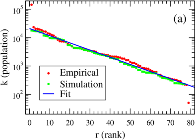
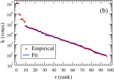
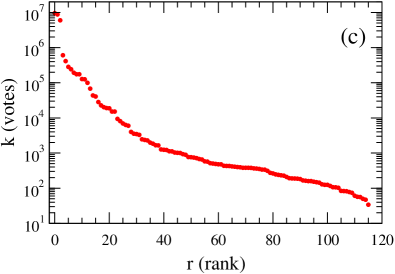
Figure 1: (colour on-line) a, rank-size distribution of the cities of the province of Huelva, Spain (2008), sorted from largest to smallest, compared with the result of a simulation with Brownian walkers (green squares). b, rank-plot of the 2008 General Elections results in Spain. c, rank-plot of the 2005 General Elections results in the United Kingdom. (red dots: empirical data; blue lines: linear fitting).

The total density distribution for $k$ is obtained integrating for all $v$ the density distribution in configuration space. Integrating  (13) we get

$$\widetilde{f}(k)=\int\rmd v\widetilde{f}(k,v)=\frac{N}{\Omega}\frac{1}{k}=\frac{\rho_{0}}{k},$$ (15)

which corresponds for large $N$ to an exponential rank-size distribution

$$k(r)=k_{1}\exp\left[\Omega-\frac{r-1}{\rho_{0}}\right],$$ (16)

where $r$ is the rank.

This behaviour, which corresponds to the class of universality $\gamma=0$ in (1), has been empirically found by Costa Filho et al. [8] in the distribution of votes in the Brazilian electoral results. We have found such a behaviour in the city-size distribution of small regions and electoral results, like the province of Huelva (Spain) [23], and the 2008 Spanish General Elections results [24], respectively. We show in figure 1a and 1b their rank-size distribution in semi-logarithmic scale, where a straight line corresponds to a distribution of type (16). Most of the distribution can be linearly fitted, with a correlation coefficient of $0.994$ and $0.998$ respectively. From these fits we have obtain a bulk density of $\rho_{0}=0.058$ for the General Elections results, and in the case of Huelva $\rho_{0}=17.1$ ($N=77$, $\Omega=4.5$). Using historical data for the latter [23], we have used the backward differentiation formula to calculate the relative growth rate of the $i$-th city as

$$w_{i}=\frac{\ln k_{i}^{(2008)}-\ln k_{i}^{(2007)}}{\Delta t}$$ (17)

where $k_{i}^{(2007)}$ and $k_{i}^{(2008)}$ are the number of inhabitants of the $i$-th city in $2007$ and $2008$ respectively and $\Delta t=1$ year. We have obtained $\overline{w}=0.012$ years^-1 and $\sigma_{w}=0.032$ years^-1. However, the regularities are not always obvious, as shown for the most voted parties in Spain’08 or the whole distribution of the 2005 General Elections results in the United Kingdom [25] (figure 1c). In both cases, the competition between parties seems to play an important role, and the assumption of non-interacting elements can be unrealistic .

4 The Zipf regime

In the previous subsection we considered that $N/\Omega$ remains finite even in the thermodynamic limit, i.e., the system reaches the bulk density $\rho_{0}$. However, if $N/\Omega\rightarrow 0$ as $\Omega\rightarrow\infty$, i.e., the system is exposed to an empty infinite volume, the normalization can not be achieved and the constraint has to be removed ($\mu=0$). We call this case the Zipf regime, in order to distinguish it from the general.

Considering only the $k$ coordinate in the domain $[k_{1},\infty)$, the information measure for the total density distribution $\widetilde{f}(k)\rmd k=f(u)\rme^{u}\rmd u=p(u)\rmd u$, reads

$$I_{u}=c_{u}\int\rmd u~{}\rme^{u}f(u)\left|\frac{\partial\ln f(u)}{\partial u}\right|^{2},$$ (18)

and the extremization problem

$$\delta\left\{c_{u}\int\rmd u~{}\rme^{u}f\left|\frac{\partial\ln f}{\partial u}\right|^{2}\right\}=0.$$ (19)

Introducing $f(u)=\rme^{-u}\Psi^{*}(u)\Psi(u)$, and varying with respect to $\Psi^{*}$ leads to the Schrödinger equation

$$\left[-4\frac{\partial^{2}}{\partial u^{2}}+1\right]\Psi(u)=0.$$ (20)

Taking the boundary conditions $\lim_{u\rightarrow\infty}f(u)=0$ and $f(u_{1})=C$ where $u_{1}=\ln k_{1}$ and $C$ is a constant, the solution to the equation is $\Psi(u)=C^{\prime}\rme^{-u/2}$, where $C^{\prime}=\sqrt{C}\rme^{u_{1}}$. It can be shown that this is just an exponential decay in $u$ space $f(u)\rme^{u}\rmd u=C\rme^{-u}\rmd u$. This solution leads to the total density distribution

$$\widetilde{f}(k)=\frac{C^{2}}{k^{2}}$$ (21)

with $C^{2}=Nk_{1}$ for a normalized density. It corresponds in the continuous limit to a rank-size distribution of the type

$$k(r)=\frac{Nk_{1}}{r},$$ (22)

which is the Zipf’s law (universal class $\gamma=1$) of  [2, 3, 4, 6, 7, 9, 10, 11]. This result is remarkable: for the first time Zipf’s law is derived from first principles.

In figure 2 we show the known behaviour [11] of the rank size distribution of the top 100 largest cities of the United States [27], which shows an slope near $-1$ ($\gamma=1$) in the logarithmic representation of the rank-plot.

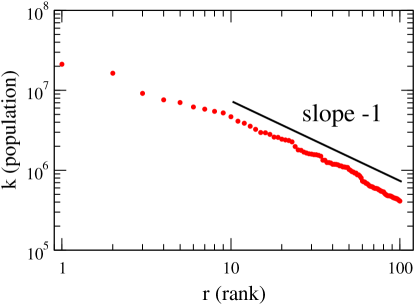
Figure 2: (colour on-line) Rank-plot of the 100 largest cities of the United States.

The appearance of the bulk and the Zipf regime in a SFIG can be understood studying empirical data. We have studied the system formed by all Physics journals [28] ($N=310$) using their total number of cites as coordinate $k$. If a journal receives more cites due to its popularity, it becomes even more popular and therefore it will receive more cites. Under such conditions proportional growth and scale invariance are expected. Since we consider all fields of Physics, correlation effects are much lower than only consider journals of an specific field, so the non-interacting approximation seems realistic in this case. In figure 3 we show the rank-plot of the number of cites of Physic journals, where we have found a slope near $-1$ for the most-cited journals in the logarithmic representation (figure 3a) and an slope near $+1$ for the less-cited journals (figure 3b). For the central part of the distribution bulk density reaches a value of $\rho_{0}\sim 57$ (figure 3c).

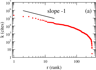
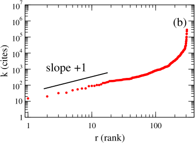
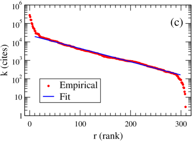
Figure 3: (colour on-line) a, rank-plot of the total number of cites of physics journal, from most-cited to less-cited, in logarithm scale. b, sorted from less-cited to most cited c, same as a, in semi-logarithm scale.(red dots: empirical data; blue line: linear fitting).

This distribution shows an extraordinary symmetric behaviour under the change $k\rightarrow 1/k$ ($u\rightarrow-u$). We show in figure 4 the raw empirical data compared with the distribution obtained from the transformation $k^{\prime}=c/k$ ($u^{\prime}=-u+\ln c$), where $c=3.3\times 10^{6}$. The symmetry of this system is an important clue to understand both regimes, and represents a perfect example of the conditions needed to observe bulk and Zipf regimes in a non-interacting scale-invariant system. The main part of the density distribution reaches the bulk density obeying (15), whereas Zipf’s law emerge at the edges, obeying (21): following the analogy with the physics of gases and fluids, we can think of the system as a drop, where the Zipf regime is the sign of a surface since it reproduces how the density exponentially falls from the bulk density to zero in $u$ space when the system is exposed to an infinite empty volume. This effect is clearly visible in figure 5, where the empirical density distribution $p(u)\rmd u$ in $u$ space is compared with the fitted density

$$p(u)=\left\{\begin{array}[]{ll}\rho_{a}\rme^{u}&\mathrm{if~{}}u<u_{a}\\ \rho_{0}&\mathrm{if~{}}u_{a}<u<u_{b}\\ \rho_{b}\rme^{-u}&\mathrm{if~{}}u_{b}>u\end{array}\right.$$ (23)

where $\rho_{a}=0.1$, $\rho_{0}=57$, $\rho_{b}=4.3\times 10^{5}$, $u_{a}=5.2$ and $u_{b}=10$. These findings lead us to conclude that the system of Physics journals sorted by total number of cites is a perfect example of the scale-free ideal gas at equilibrium.

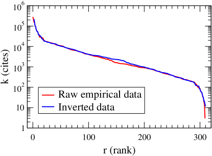
Figure 4: (colour online) Rank-plot of the total number of cites of Physics journal, from most-cited to less-cited, compared with the distribution obtained from the inverse transformation $k^{\prime}=3.3\times 10^{6}/k$ where $k$ is the number of cites.

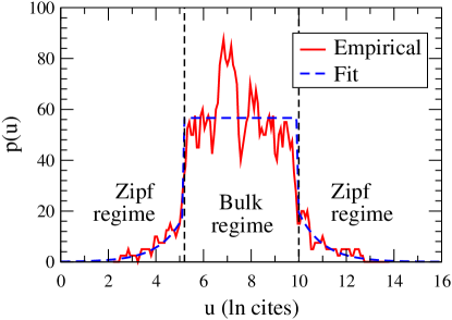
Figure 5: (colour online) Empirical density distribution in $u$ space of the total number of cites of Physics journals, compared with  (23). The bulk regime and the Zipf regime at the edges is clearly visible.

5 The harmonically constrained system

We now consider a system with a constraint in a given observable $\langle A\rangle$ which locally depends on $k$, $A=A(k)$. The second order Taylor expansion with respect to $u=\ln k$ near a minimum is written as $\widetilde{A}(u)=A(\rme^{u})\simeq A_{0}+A_{2}/2(u-u_{m})^{2}$, where $A_{0}$, $A_{2}$ and $u_{m}$ are constants. Introducing this constraint and the normalization condition to the number of elements $N$ of the total density distribution, the extremization problem reads

$$\begin{array}[]{rl}\delta&\displaystyle\left\{c_{u}\int\rmd u~{}\rme^{u}f\left|\frac{\partial\ln f}{\partial u}\right|^{2}+\mu\int\rmd u~{}\rme^{u}f\right.\\ &\displaystyle\left.+\lambda\int\rmd u~{}\rme^{u}f\left[A_{0}+\frac{1}{2}A_{2}(u-u_{m})^{2}\right]\right\}=0\end{array}$$ (24)

Introducing $f(u)=\rme^{-u}\Psi^{*}(u)\Psi(u)$, and varying with respect to $\Psi^{*}$ leads to the quantum harmonic oscillator equation

$$\left[-4\frac{\partial^{2}}{\partial u^{2}}+\lambda^{\prime}(u-u_{0})^{2}+\nu^{\prime}\right]\Psi(u)=0,$$ (25)

where now we have defined $\lambda^{\prime}=(\lambda A_{2})/2c_{w}$ and $\nu^{\prime}=(\nu+1+\lambda A_{0})/c_{u}$. The ground state solution is a gaussian distribution, which now yields a total density distribution of the form of a log-normal distribution

$$\widetilde{f}(k)=\frac{N}{k\sqrt{2\pi}\sigma_{u}}\exp\left(\frac{-(\ln k-u_{m})^{2}}{2\sigma_{u}^{2}}\right),$$ (26)

with $|\lambda^{\prime}|^{-1/2}=\sigma_{u}^{2}=\langle A\rangle-A_{0}$. Note that if $A_{0}=0$, the constraint can be also understood as a constraint in the variance of $u$.

The log-normal distribution has been widely observed in a large number of scale-invariant systems [29]. In [30] S. Fortunato and C. Castellano found this behaviour in the electoral results of different countries and for different years. We can think of this constraint as the effect of polices or social factors: low popularity candidates are penalized since the party does not present them for the elections, and high popularity candidates are penalized by the competition in campaign. Both effects can be approximated to second order as a harmonic potential, however anharmonic effects are expected in a high order study.

Defining $H^{\prime\prime}=1/\Delta\tau$ and $k_{m}=\ln u_{m}$ being $k_{m}=m\Delta k$, the entropy equation of state reads in this case

$$S=N\kappa\left\{\ln\frac{2\pi\sigma_{u}\sigma_{w}m^{2}}{NH^{\prime\prime}}+2\right\},$$ (27)

which maintains scale invariance.

6 The microscopic description

The dynamics of the system can be microscopically described as a stochastic process using (4) and the density distribution (12). Treating $w$ as a random variable, the stochastic equation of motion is written as a geometrical Brownian motion

$$\rmd k=k\overline{w}\rmd t+k\sigma_{w}\rmd W,$$ (28)

where $\rmd W$ is a Wiener process. In the $u$ space, this equation reads

$$\rmd u=\overline{w}\rmd t+\sigma_{w}\rmd W,$$ (29)

which describes the well-known Brownian motion. (28) exactly describes the dynamical condition found empirically in  [7] and also the stochastic proportional growth model used in [11] to obtain Zipf’s law. We can think of this sort of simulations as the equivalent of molecular dynamics simulations for gases and liquids [31].

Effectively, (29) implies that a uniform density in $u$ space of $N$ Brownian walkers moving in a fixed volume $\Omega$ —a model used in the literature to describe the IG [31]— describes the SFIG when we represent the system with the coordinates $(k,v)$. In figure 1a we show the rank-plot for a system of $N=78$ geometrical Brownian walkers with $\sigma_{w}=0.029$ in a volume of $\Omega=4.5$ and $k_{1}=200$ in reduced units, which nearly describes the distribution of the population of the province of Huelva.

7 Summary and Discussion

We have shown that a thermodynamic description of scale-invariant systems can be formulated from the principle of extreme information, finding an analogy with the thermodynamics of gases and fluids. We have derived the density distribution in configuration space and the entropy equation of state of the scale-free ideal gas in the thermodynamic limit, and have found empirical evidences of its existence in city population, electoral results and cites to Physics journals. In this context, Zipf’s law emerges naturally as the equilibrium density of the non-interacting system when the volume grows to infinity, what we call the Zipf regime. Using empirical data we have seen that this regime can be understood as the density fall of a surface between the bulk and an empty volume. We have also studied the effect of a harmonic constraint, finding that in this case the density of the system follows a log-normal distribution, which has been empirically observed in electoral results and in many other scale-invariant systems [29]. Finally we have shown with a simulation of city population that a geometrical Brownian motion can describe the system at a microscopic level.

It is well known that in real gases the most interesting situations emerge when interactions between particles become relevant, originating deviations from the equation of state of the IG, and making room for the appearance of, e.g., phase transitions [21]. Analogously, one should also expect this rich phenomenology to show up in scale-invariant real systems, which may explain deviations from Zipf’s law in empirical distributions. A study beyond the ideal gas is in progress, and further results will be reported [26].

Appendix A The translational invariant ideal gas

In this appendix we derive from the principle of extreme information the density distribution in configuration space and the entropy equation of state of the translational invariant ideal gas (IG) [21]. The IG model describes non-interacting classical particles of mass $m$ with coordinates $\bi{q}=(\bi{r},\bi{p})$, where $m\rmd\bi{r}/\rmd t=\bi{p}$. We assume that these coordinates are canonical [22] and uncorrelated. This assumption is introduced in the information measure (2) as $c_{ij}=c_{i}\delta_{ij}$, where $c_{i}=c_{r}$ for space coordinates, $c_{i}=c_{p}$ for momentum coordinates, and $\delta_{ij}$ is the Kronecker delta. The density distribution can be factorized as $f(\bi{r},\bi{p})=\rho(\bi{r})\eta(\bi{p})$, and the information measure $I=I_{r}+I_{p}$ reads, if $D$ is the dimension of the space

$$\begin{array}[]{rl}I_{r}=&\displaystyle c_{r}\int\rmd^{D}\bi{r}~{}\rho(\bi{r})\left|\bi{\nabla}_{r}\ln\rho(\bi{r})\right|^{2}\\ I_{p}=&\displaystyle c_{p}\int\rmd^{D}\bi{p}~{}\eta(\bi{p})\left|\bi{\nabla}_{p}\ln\eta(\bi{p})\right|^{2}.\end{array}$$ (30)

In the extremization of Fisher information we constrain the normalization of $\rho(\bi{r})$ and $\eta(\bi{p})$ to the total number of particles $N$ and to $1$, respectively

$$\int\rmd^{D}\bi{r}~{}\rho(\bi{r})=N,\qquad\int\rmd^{D}\bi{p}~{}\eta(\bi{p})=1.$$ (31)

In addition, we penalize infinite values for the particle momentum with a constraint on the variance of $\eta(\bi{p})$ to a given measured value

$$\int\rmd^{D}\bi{p}~{}\eta(\bi{p})(\bi{p}-\overline{\bi{p}})^{2}=D\sigma_{p}^{2},$$ (32)

where $\overline{\bi{p}}$ is the mean value of $\bi{p}$. For each degree of freedom it is known from the Virial theorem that the variance is related to the temperature $T$ as $\sigma_{p}^{2}=mk_{B}T$, being $k_{B}$ the Boltzmann factor. The variation yields

$$\delta\left\{c_{r}\int\rmd^{D}\bi{r}~{}\rho\left|\bi{\nabla}_{r}\ln\rho\right|^{2}+\mu\int\rmd^{D}\bi{r}~{}\rho\right\}=0$$ (33)

and

$$\delta\left\{c_{p}\int\rmd^{D}\bi{p}~{}\eta\left|\bi{\nabla}_{p}\ln\eta\right|^{2}+\lambda\int\rmd^{D}\bi{p}~{}\eta(\bi{p}-\overline{\bi{p}})^{2}+\nu\int\rmd^{D}\bi{p}~{}\eta\right\}=0,$$ (34)

where $\mu$, $\lambda$ and $\nu$ are Lagrange multipliers.

Introducing $\rho(\bi{r})=\Psi^{*}(\bi{r})\Psi(\bi{r})$ and varying (33) with respect to $\Psi^{*}$ leads to the Schrödinger equation [18]

$$\left[-4\nabla_{r}^{2}+\mu^{\prime}\right]\Psi(\bi{r})=0,$$ (35)

where $\mu^{\prime}=\mu/c_{r}$. To fix the boundary conditions, we first assume that the $N$ particles are confined in a box of volume $V$, and next we take the thermodynamic limit (TL) $N,V\rightarrow\infty$ with $N/V$ finite. The equilibrium state compatible with this limit corresponds to the ground state solution, which is the uniform density $\rho(\bi{r})=N/V$.

Introducing $\eta(\bi{p})=\Phi^{*}(\bi{p})\Phi(\bi{p})$ and varying (34) with respect to $\Phi^{*}$ leads to the quantum harmonic oscillator equation [18]

$$\left[-4\nabla_{p}^{2}+\lambda^{\prime}(\bi{p}-\overline{\bi{p}})^{2}+\nu^{\prime}\right]\Phi(\bi{p})=0,$$ (36)

where $\lambda^{\prime}=\lambda/c_{p}$ and $\nu^{\prime}=\nu/c_{p}$. The equilibrium configuration corresponds to the ground state solution, which is now a gaussian distribution. Using (32) to identify $|\lambda^{\prime}|^{-1/2}=\sigma_{p}^{2}$ we get the Boltzmann distribution, which leads to a density distribution in configuration space of the form

$$f(\bi{r},\bi{p})=\frac{N}{V}\frac{\exp\left[-(\bi{p}-\overline{\bi{p}})^{2}/2\sigma_{p}^{2}\right]}{(2\pi\sigma_{p}^{2})^{D/2}}.$$ (37)

If $H$ is the elementary volume in phase space, the total number of microstates is $Z=N!H^{DN}\prod_{i=1}^{N}f_{1}(\bi{r}_{i},\bi{p}_{i})$, where $f_{1}=f/N$ is the monoparticular distribution and $N!$ counts all possible permutations for distinguishable particles. The entropy $S=-k_{B}\ln Z$ is written as

$$S=Nk_{B}\left\{\ln\frac{V}{N}\left(\frac{2\pi\sigma_{p}^{2}}{H^{2}}\right)^{D/2}+\frac{2+D}{2}\right\},$$ (38)

where we have used the Stirling approximation for $N!$. This expression is in exact accordance with the known value of the entropy for the IG [21], which shows the predictive power of the Fisher formulation.

References

References

- [1] Fractals in Physics, edited by Aharony A and Feder J 1989 Proc. Conf. in honor of Mandelbrot B B, Vence, France (North Holland, Amsterdam).
- [2] Paech K, Bauer W and Pratt S 2007 Phys. Rev. C 76, 054603; Campi X and Krivine H 2005 Phys. Rev. C 72, 057602 ; Ma Y G et al. 2005 Phys. Rev. C 71, 054606.
- [3] Furusawa C and Kaneko K 2003 Phys. Rev. Lett. 90, 088102.
- [4] Zipf G K 1949 Human Behavior and the Principle of Least Effort (Addison-Wesley Press, Cambridge, Mass.); Kanter I and Kessler D A 1995 Phys. Rev. Lett. 74, 4559.
- [5] Newman M E J 2001 Phys. Rev. E 64, 016131.
- [6] Barabasi A L and Albert R 2002 Rev. Mod. Phys. 74, 47
- [7] Maillart T, Sornette D, Spaeth S and von Krogh G 2008 Phys. Rev. Lett. 101, 218701.
- [8] Costa Filho R N, Almeida M P, Andrade J S and Moreira J E 1999 Phys. Rev. E 60, 1067.
- [9] Malacarne L C, Mendes R S and Lenzi E K 2001 Phys. Rev. E 65, 017106; Marsili M and Zhang Yi-Cheng 1998 Phys. Rev. Lett. 80, 2741.
- [10] Axtell R L 2001 Science 293, 1818.
- [11] Gabaix X 1999 Quarterly Journal of Economics 114, 739.
- [12] Kechedzhi K E, Usatenko O V and Yampol’skii V A 2005 Phys. Rev. E. 72, 046138; Ree S 2006 Phys. Rev. E. 73, 026115.
- [13] Moreira A A, Paula D R, Costa Filho R N and Andrade J S 2006 Phys. Rev. E 73, 065101(R).
- [14] Reed W J and Hughes B D 2002 Phys. Rev. E. 66, 067103.
- [15] Frieden B R, Plastino A, Plastino A R and Soffer B H 1999 Phys. Rev. E 60, 48; 2002 Phys. Rev. E 66, 046128.
- [16] Pennini F, Plastino A, Soffer B H and Vignat C 2009 Phys. Let. A 373, 817.
- [17] Frieden B R and Soffer B H 1995 Phys. Rev. E 52, 2274; Frieden B R 1998 Physics from Fisher Information, 2nd Ed. (Cambridge Univ. Press, Cambridge); Frieden B R 2004 Science from Fisher Information (Cambridge Univ. Press, Cambridge).
- [18] Cohen-Tannoudji C, Diu B and Laloe F 2006 Quantum Mechanics (Wiley-Interscience, New York).
- [19] Pennini F and Plastino A 2006 Phys. Lett. A 349, 15.
- [20] Frieden B R and Gatenby R A 2005 Phys. Rev. E 72, 036101.
- [21] Zemansky M W and Dittmann R H 1981 Heat and Thermodynamics(McGraw-Hill, London).
- [22] Goldstein H, Poole C and Safko J 2002 Classical Mechanics 3rd Ed. (Addison Wesley, San Francisco).
- [23] National Statistics Institute, Spain, www.ine.es.
- [24] Ministry of the Interior, Spain, www.elecciones.mir.es
- [25] Electoral Commission, Government of the UK, www.electoralcommission.org.uk.
- [26] Hernando A, Villuendas D, Abad M and Vesperinas C (2009) arXiv:0905.3704v1 [cond-mat.stat-mech]
- [27] Census bureau website, Government of the USA, www.census.gov.
- [28] Journal Citation Reports (JCR) for 2007, Thomson Reuters
- [29] Limpert E, Stahel W and Abbt M 2001 BioScience, 51, 341.
- [30] Fortunato S and Castellano C 2007 Phys. Rev. Lett., 99, 138701.
- [31] Gould H and Tobochnik J 1996 An Introduction to Computer Simulation Methods: Applications to Physical Systems, 2nd Ed. (Addison-Wesley).