Physical conditions in the ISM of intensely star-forming galaxies at redshift$\sim$2

Abstract

We analyze the physical conditions in the interstellar gas of 11 actively star-forming galaxies at z$\sim$2, based on integral-field spectroscopy from the ESO-VLT and HST/NICMOS imaging. We concentrate on the high H$\alpha$ surface brightnesses, large line widths, line ratios and the clumpy nature of these galaxies. We show that photoionization calculations and emission line diagnostics imply gas pressures and densities that are similar to the most intense nearby star-forming regions at z=0 but over much larger scales (10-20 kpc). A relationship between surface brightness and velocity dispersion can be explained through simple energy injection arguments and a scaling set by nearby galaxies with no free parameters. The high velocity dispersions are a natural consequence of intense star formation thus regions of high velocity dispersion are not evidence for mass concentrations such as bulges or rings. External mechanisms like cosmological gas accretion generally do not have enough energy to sustain the high velocity dispersions. In some cases, the high pressures and low gas metallicites may make it difficult to robustly distinguish between AGN ionization cones and star formation, as we show for BzK-15504 at z$=$2.38. We construct a picture where the early stages of galaxy evolution are driven by self-gravity which powers strong turbulence until the velocity dispersion is high. Then massive, dense, gas-rich clumps collapse, triggering star formation with high efficiencies and intensities as observed. At this stage, the intense star formation is likely self-regulated by the mechanical energy output of massive stars.

1. Introduction

Elucidating the physical processes that regulate global star formation is one of the keys to understanding galaxy evolution. The power-law relation, over several orders of magnitude, between the warm HI and cold molecular gas surface density and star formation intensity (“Schmidt-Kennicutt law”) is telling us that there must be underlying physical processes that control and regulate star formation (e.g., Kennicutt et al., 2007). However, with a myriad of possible mechanisms for regulating star formation over large scales – cloud formation and destruction, mechanical energy output from stars and AGN, spiral density waves, turbulence induced by gravity and mechanical energy, magnetic fields, mixing layers, and many others – it is challenging to distill a unifying explanation over many orders of magnitudes in gas density. One possible way of advancing our understanding of the processes that regulate global star formation is by studying the most extreme star-forming galaxies locally and at cosmological distances (e.g., Lehnert & Heckman, 1996a; Shapley et al., 2003; Verma et al., 2007).

Thanks to recent technological improvements, we are now able to study the basic physical processes driving galaxy assembly directly and over large ranges of cosmic time. In particular, the number of galaxies at redshifts of 2$-$3 with detailed integral-field spectroscopic studies in the rest-frame optical is still small, less than a few dozen, but growing rapidly. These observations allow us to trace spatially resolved emission-line properties, and to investigate galaxy kinematics and the physical conditions of the ionized gas. Up to now, most studies have focused on the kinematic properties of the galaxies and less so on the properties of the emission lines themselves beyond their relative velocities and widths. Recombination line fluxes were used to estimate star-formation rates using simple prescriptions developed for low-redshift galaxies (Genzel et al., 2006; Förster Schreiber et al., 2006; van Starkenburg et al., 2008; Law et al., 2007; Wright et al., 2007; Nesvadba et al., 2008a).

With these estimates and assumptions, far-reaching conclusions have been made regarding the modes of galaxy assembly and the drivers of star formation in the early Universe. Many of these studies (e.g., Genzel et al., 2006; Förster Schreiber et al., 2006) favor a scenario where high-redshift galaxies exhibit gaseous disks of $\sim$10-20 kpc in size, which, unlike galaxies at low redshift, are dynamically hot with large gas velocity dispersions, $\sigma$, relative to their bulk velocities, $v$ (see also Nesvadba et al., 2006a). The ratios of random to large scale velocity shear at high redshift are of order v/$\sigma\sim$few, compared to v$/\sigma\geq 10$ at low redshift. To explain these observations, Kereš et al. (2005, 2008); Ocvirk et al. (2008); Dekel et al. (2009b) proposed a scenario where galaxies at z$\sim 2$ accrete significant amounts of cold gas, which after accumulating and forming gaseous disks, will become gravitationally unstable and lead to the observed high star formation rates (Genzel et al., 2008; Dekel et al., 2009b). In this picture, mergers and hydrodynamic processes like feedback from star formation and AGN play only a minor role in assembling early galaxies, beginning to play a significant role only as a consequence of the build-up of the bulk of the stellar mass in bulges and disks.

Given the faintness of the targets and the often low number of diagnostic optical emission lines, usually only studying H$\alpha$ or [OIII]$\lambda$5007, many of these results must rely on the assumption that the gas conditions in the interstellar medium will overall be largely similar to those in galaxies at low redshift. This assumption has not been tested directly on the observed properties of high-redshift galaxies.

We already know of (or may plausibly expect) several major differences between galaxies at high and at low redshift, which may strongly influence the state of their interstellar medium and thus, their rest-frame optical line emission. First, many galaxies at high redshift are less evolved, with higher fractions (Erb et al., 2006c) of lower-metallicity gas (Erb et al., 2006a; Maiolino et al., 2008). This may have rather subtle observational consequences. For example, Robertson & Bullock (2008) discuss the expected morphology of an advanced (or mostly relaxed) merger of two gas-rich disk galaxies as would be observed using state-of-the-art Integral-Field Units (IFUs). They find that their model reproduces the observed properties of high redshift galaxies as well as pure (and isolated) disk models, which are often favored by observers in contrast to on-going or advanced mergers (Nesvadba et al., 2006a; Genzel et al., 2006, 2008; Wright et al., 2008).

Second, virtually all high-redshift galaxies studied in detail with IFUs have very high surface brightnesses of the recombination lines. Given the impact of cosmological surface brightness dimming, which is a strong function of redshift ($\propto(z+1)^{4}$ for bolometric luminosities and spectral lines, $\propto(z+1)^{5}$ for broadband photometry due to the additional ’stretching’ of the continuum; see, e.g., Tolman, 1930), and current observational limits, all observations at high redshift will naturally be biased towards the most luminous emission-line regions, and the most luminous galaxies. As a result, all galaxies so far studied with IFUs have star-formation rates of several 10s of M_☉ yr^-1 or more, and typical star-formation intensities, $SFI$, well above the critical threshold of SFI${}_{crit}\sim$ 0.1 M_☉ yr^-1 kpc^-2(Heckman, 2003) necessary to drive vigorous outflows in local galaxies. Galaxies with $SFI\mathrel{\hbox{\hbox to0.0pt{\hbox{\lower 4.0pt\hbox{$\sim$}}\hss}\hbox{$>$}}}SFI_{crit}$ are observed to create and maintain strongly over-pressurized bubbles of hot gas from the thermalized ejecta of supernovae and massive young stars, which expand perpendicular to the disk plane and produce galactic-scale outflows (Heckman et al., 1990; Lehnert & Heckman, 1996a, b). These outflows may play an important role in rendering a starburst “self-regulating” (Dopita & Ryder, 1994; Silk, 1997). The observational signatures of starburst-driven winds, such as characteristic velocity offsets between the rest-frame UV absorption lines and the systemic velocity (Pettini et al., 2000; Erb et al., 2004, 2006a), or blue wings in rest-frame optical emission lines (e.g. Nesvadba et al., 2007), are commonly observed at high redshift. In a detailed study of a massive, z$\sim 2.6$ starburst and the related outflow of a submillimeter-selected galaxy at z$\sim 2.6$, Nesvadba et al. (2007) found that overall, the physical properties of maximal starbursts at z$\sim$2$-$3 appear very similar to local starbursts. The starburst appears to be self-regulating, and characteristic, density-sensitive line ratios suggest that the pressures in the starburst region, which are ultimately driving the observed outflow, are very similar to those in low-redshift starbursts.

This may have a non-negligible impact on our interpretation of the physical processes in high-redshift galaxies, because much of our well-established low-redshift emission line diagnostics relies on the physical gas conditions in rather subtle ways. For example, when relating the ratios of strong, low-ionization nebular emission lines with H$\alpha$, like, [Nii]/H$\alpha$, [Oi]/H$\alpha$, or [Sii]/H$\alpha$ with the [Oiii]/H$\beta$ ratios, starburst galaxies will fall onto a characteristic curve (Baldwin et al., 1981; Veilleux & Osterbrock, 1987), whereas AGN will fall into a different part of the diagram. For high-redshift galaxies, however, the same relationship may not be strictly valid. Erb et al. (2006a) observed that, although UV selected galaxies at z$\sim 2$ follow the overall shape of the starburst-curve in the [Nii]/H$\alpha$ versus [Oiii]/H$\beta$ diagram, as a whole, they are offset towards larger [Nii] fluxes. Brinchmann et al. (2008) collected a comparison sample of low-redshift SDSS galaxies with similar offsets, and found that these galaxies also had statistically higher H$\alpha$ equivalent widths. They argue that the most likely explanation may be higher ionization parameters and densities in high-redshift star-forming regions compared to local galaxies. We will further develop these arguments and illustrate that pressures induced by the starbursts may very naturally explain some of the kinematic properties of high-redshift galaxies as well.

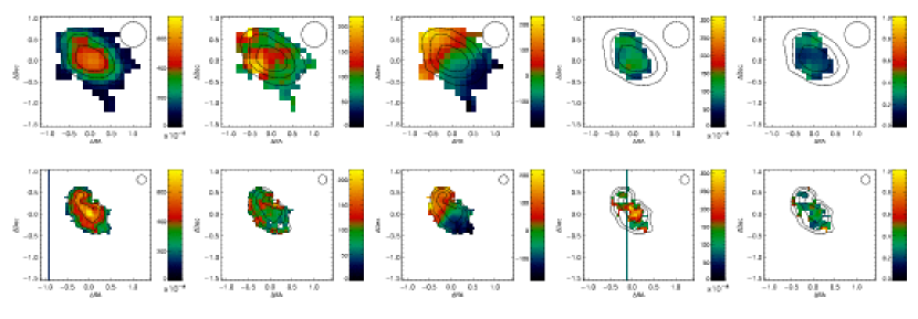
Figure 1.— The various emission line and kinematic maps for the source, ZC782941, used in our analysis. (top row and from left to right) The H$\alpha$ flux, velocity dispersion, velocity, [NII]$\lambda$6583, and [NII]$\lambda$6583/H$\alpha$ ratio maps respectively for the 250 mas (non-AO assisted) data for ZC782941. (bottom row) The maps of ZC782941 in the same order as for the top row but now for the observations taken with the 100 mas pixel scale and with the assistance of adaptive optics. In each of the panels, we show the approximately size of the full-width at half-maximum of the seeing disk (the disk marked “seeing” in each plot) and the relative positions are in arc seconds. The contours in each maps are the distribution of the H$\alpha$ emission in each of the two cubes (with the lowest contour and step between contours of 1.4 $\times$ 10^-16 erg s^-1 cm^-2 arcsec^-2 for the non-AO assisted data and 1.7 $\times$ 10^-16 erg s^-1 cm^-2 arcsec^-2 for the AO assisted data). All maps were centered on the peak in the H$\alpha$ surface brightness distribution which defines the (0,0) in each panel.

However, the line ratios indicative of excitation by an AGN may also shift at high redshift (Groves et al., 2006). Since most luminous AGN at low redshift preferentially reside in massive galaxies (e.g., Kauffmann et al., 2003), and because gas metallicity correlates with galaxy mass (e.g., Tremonti et al., 2004), most AGN hosts at low redshift will have narrow-line regions with high metallicities. Groves et al. (2006) modeled the diagnostic line ratios for AGN in relatively low-metallicity host galaxies. They showed that star-formation plus AGN in relatively low metallicity host galaxies could explain the offset observed for example by Erb et al. (2006a). We will show that many z$\sim 2-3$ galaxies fall very close to these regions, which may make it difficult to robustly quantify the role of AGN and starbursts in exciting the optical emission line gas.

We will in the following present an analysis of 11 galaxies with particularly deep near-infrared integral-field spectroscopy obtained at the VLT. These data allow in particular to trace intrinsically fainter nebular emission lines such as [Oi]$\lambda$6300 and [Sii]$\lambda\lambda$6716,6731 which being close in wavelength to H$\alpha$ often fall into the same band. A subset of 5 galaxies also have measurements of the [Oiii]$\lambda$4959,5007 and H$\beta$ lines, which fall into the near-infrared H band, and which have not been discussed previously in the literature. Many of the arguments in previous papers are based on the implicit assumption that most of the emission originates from “ordinary” Hii regions similar to low-redshift disk galaxies and thus, that observations of the warm ionized gas are representative of all of the kinematics and other properties of the phases of the ISM. In contrast, our analysis is aimed at quantifying the physical conditions in the interstellar medium of these galaxies principally by investigating the surface brightnesses of the recombination lines, various optical emission line ratios, and line widths to test this underlying assumption.

Throughout the paper we adopt a flat H${}_{0}=$70 km s^-1 Mpc^-3 concordance cosmology with $\Omega_{\Lambda}=0.7$ and $\Omega_{M}=0.3$.

2. Observations and data reduction

For our analysis of the physical conditions in the interstellar medium of strongly star-forming, high-redshift galaxies, we collected a sample of 11 galaxies at z$\sim$1.5$-$2.5 from the SINS program (Förster Schreiber et al., 2006) with rest-frame optical integral-field spectroscopy (Table 1).

Data were taken with the near-infrared integral-field spectrograph SINFONI on the ESO Very Large Telescope in several runs between 2004 and 2006. Observations have been presented elsewhere (Förster Schreiber et al., 2006; Genzel et al., 2008). We reduced these data independently from any other previous work, using the IRAF (Tody, 1993) standard tools for the reduction of longslit spectra, modified to meet the special requirements of integral-field spectroscopy, and complemented by a dedicated set of IDL routines. Data are dark-frame subtracted and flat-fielded. The position of each slitlet is measured from a set of standard SINFONI calibration data, measuring the position of an artificial point source. Rectification along the spectral dimension and wavelength calibration are done before night sky subtraction to account for some spectral flexure between the frames. Curvature is measured and removed using an arc lamp, before shifting the spectra to an absolute (vacuum) wavelength scale with reference to the OH lines in the data. To account for variations in the night sky emission, we normalize the sky frame to the average of the object frame separately for each wavelength before sky subtraction, correcting for residuals of the background subtraction and uncertainties in the flux calibration by subsequently subtracting the (empty sky) background separately from each wavelength plane. These data reduction procedures have fewer interpolations and are optimized for faint, extended, low surface brightness objects compared to the SINFONI pipeline which obviously must be capable of reducing a much wider variety of objects. Overall, we expect that these differences lead to more robust data compared to previous reductions but overall the results are largely consistent.

The three-dimensional data are then reconstructed and spatially aligned using the telescope offsets as recorded in the header within the same sequence of dithered exposures (about one hour of exposure), and by cross-correlating the line images from the combined data in each sequence, to eliminate relative offsets between different sequences. Telluric correction is applied to each final cube. Flux scales are obtained from standard star observations taken every hour at similar position and air mass as the source.

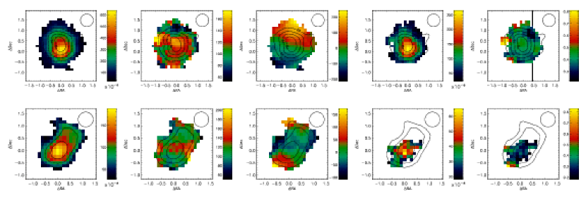
Figure 2.— The various emission line and kinematic maps for the source, Q2343-BX610 and Q2343-BX528, used in our analysis. We show these two sources for comparison with previously published maps in the literature. (top row and from left to right) The H$\alpha$ flux, velocity dispersion, velocity, [NII]$\lambda$6583, and [NII]$\lambda$6583/H$\alpha$ ratio maps respectively for the for Q2343-BX610. (bottom row) The maps of Q2343-BX528 in the same order as for the top row. In each of the panels, we show the approximately size of the full-width at half-maximum of the seeing disk (the disk marked “seeing” in each plot) and the relative positions are in arc seconds. The contours for the maps of Q2343-BX610 represent the continuum, while those of Q2343-BX528 represent the H$\alpha$ surface brightness (with the lowest contour and step between contours of 4 $\times$ 10^-17 erg s^-1 cm^-2 arcsec^-2). All maps were centered on the peak in the H$\alpha$ surface brightness distribution which defines the (0,0) in each panel.

We also used the standard stars to monitor the seeing during observations, and we find an effective seeing in the combined cubes of typically FWHM $0^{\prime\prime}\,.\hskip 0.28453pt5$$-$$0^{\prime\prime}\,.\hskip 0.28453pt8$. The spectral resolution was measured from night-sky lines and is FWHM$\sim$ 115 and 150 km s^-1 in the K and H-bands, respectively, for the 250 mas pixel scale (“mas” is milli-arcseconds). In addition, for two of the sources, data were taken with adaptive optics assistance which yielded a seeing about 200 mas. The data were taken with the 100 mas pixel scale in SINFONI. In Fig. 1 we show an example of various maps that have not been presented previously for the source, ZC782941. In addition, we show example maps of the sources, Q2343-BX610 and Q2343-BX528 for comparison with previously published maps (e.g., Förster Schreiber et al., 2006). In our subsequent analysis, we will analyze the integrated H-band spectra of the sources when they are available. We show an example of the H and K-band integrated spectra for the source, Q2343-BX610, in Fig. 3.

In addition, we reduced publicly available HST/NICMOS images of 5 of the galaxies in our sample, which were observed as part of proposal ID 10924 (P.I. Shapley). Each galaxy was observed for 4 orbits using the NIC2 camera with the F160W (H-band) filter and a pixel scale of $0^{\prime\prime}\,.\hskip 0.28453pt075$. The calibrated individual exposures (_cal files) were downloaded from the HST archive and reduced using the standard IRAF routines pedsky, to correct the well-studied pedestal effect caused by residual bias, and multidrizzle, to combine the exposures. Images were corrected for the impact of additional cosmic ray events during passage through the South Atlantic Anomaly when required. The resulting images are shown in Fig. 4.

3. The remarkably high H$\alpha$ surface brightnesses and trends

In this section, we will discuss the emission line properties of our sample of galaxies such as surface brightnesses, the relationship between the velocity dispersion and surface brightness, and the impact of “beam smearing”. This analysis will form the basis of our subsequent discussion. We refer the reader to Förster Schreiber et al. (2006), Genzel et al. (2006), and Genzel et al. (2008) for a discussion of the overall kinematic properties of the galaxies in our sample.

3.1. H$\alpha$ surface brightness

One of the most remarkable, but so far little discussed, observational findings of z$\sim 2-3$ galaxies studied with IFUs are their high emission line surface brightnesses. In our sample we measure H$\alpha$ surface brightnesses of $\sim$10${}^{-15.1}-10^{-16.9}$ erg cm^-2 s^-1 arcsec^-2 (Fig. 5). The data were smoothed by 3$\times$3 pixels, i.e., averaged in areas of size $0^{\prime\prime}\,.\hskip 0.28453pt375$$\times$$0^{\prime\prime}\,.\hskip 0.28453pt375$, which is appropriate since the spatial resolution is typically $\sim$ $0^{\prime\prime}\,.\hskip 0.28453pt5$-$0^{\prime\prime}\,.\hskip 0.28453pt6$ or $\sim$4$-$5 pixels. Correcting for cosmological surface brightness dimming, this corresponds to a typical rest-frame surface brightness of 10${}^{-13.2}-10^{-14.8}$ erg cm^-2 s^-1$\sq\arcsec$ (Fig. 6). This represents a lower limit to the highest intensity regions, due to the “beam smearing” effect of the low spatial resolution of our data. In fact, for two of the galaxies, we can further quantify the effect of beam smearing on both the surface brightness distribution and line widths. For BzK-15504 and ZC782941, where we have both adaptive optics assisted and seeing limited observations, we find that the offset in surface brightness between both sets of observations is typically more than a factor of 3 (Fig. 7). This factor is similar to the ratio of the area of the point spread function in both sets (the full width half maximum of the seeing disk is typically about $0^{\prime\prime}\,.\hskip 0.28453pt5$ for the seeing limited data versus about $0^{\prime\prime}\,.\hskip 0.28453pt2$ in the AO assisted data), suggesting that the star-forming clumps are at best marginally resolved in either data set. Much of the structure must be smaller than about 2 kpc, the physical resolution of our highest resolution data. Moreover, this implies that all of the measured surface brightnesses of the most intense H$\alpha$ emission regions are under-estimated, even in the AO-assisted observations.

Figure 3.— The integrated spectrum of Q2343-BX610 in the H-band (left) and the K-band (right). All of the strong optical lines are indicated.

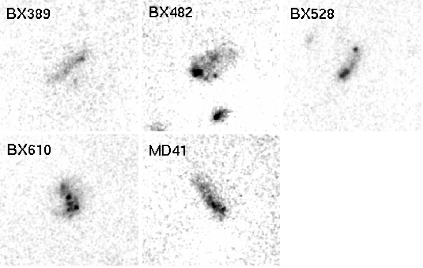
Figure 4.— HST/NICMOS NIC2 H-band (F160W) images of 5 galaxies within the sample. Images are 5$\times$5^′′, and North is at the top and East is on the left. The images have a pixel scale of 30 mas (the drizzled pixel size) and each image reaches a depth of about 28.6-28.7 m_AB pixel^-1 (for a NICMOS pixel scale of 76 mas) or about 25.8-25.9 m_AB arcsec^-2.

An H$\alpha$ surface brightness comparison between galaxies in the local and distant Universe illustrates the exceptional nature of the galaxies in our sample. Galaxies that reach the highest surface brightnesses we observe and over similar physical scales do not exist at low redshift. In a study of 84 Virgo cluster and isolated spiral galaxies, many galaxies reach surface brightness levels at the low end of what we have observed at high redshift ($\log\rm SB_{H\alpha}\mathrel{\hbox{\hbox to0.0pt{\hbox{\lower 4.0pt\hbox{$\sim$}}\hss}\hbox{$<$}}}-14$ erg cm^-2 arcsec^-2) but only in their nuclei and on scales about or less than 1 kpc (Koopmann et al., 2006a; Koopmann & Kenney, 2006b, 2004a, 2004b; Koopmann et al., 2001). Local starburst galaxies can reach higher surface brightnesses (but not as high as our peak surface brightnesses, Lehnert & Heckman, 1995, 1996a) but again only in regions that are nuclear or circum-nuclear with sizes $\mathrel{\hbox{\hbox to0.0pt{\hbox{\lower 4.0pt\hbox{$\sim$}}\hss}\hbox{$<$}}}$ 1 kpc (and well within the “turn-over” radius of the rotation curve; Lehnert & Heckman, 1996b). Even in the more extreme starburst sample of Armus et al. (1989, 1990), only a handful of galaxies reach surface brightnesses sufficient to be observed at z$\sim$2 (such as M82). At high redshift, H$\alpha$ surface brightnesses as extreme as those found only in the nuclei of nearby galaxies on small scales are found over significantly larger isophotal radii of order 10-20 kpc and are generally more extreme. Although our comparison includes some of the most powerful and intense starbursts in the local Universe, they generally do not reach sufficiently high surface brightnesses over large enough areas to correspond to any of the galaxies in our distant galaxy sample. Moreover, at the 4$-$5 kpc resolution of our seeing limited high-redshift data, none of the local starbursts would reach these maxima in the surface brightnesses that are observed due to the heavy spatial smoothing and dilution by regions with lower surface brightness.

This lack of correspondence renders any simple analogy between “ordinary” quiescently star-forming spiral galaxies in the local Universe and galaxies at z$\sim$2 questionable. Possible significant differences include the distribution of mass in various phases of the ISM, of density, of star-formation intensity, of gas fraction, and many more. Moreover, this lack implies that we cannot only study the kinematics of z$\sim$2 galaxies without investigating the nature of the physical processes that power their high surface brightness line emission, and the impact such a finding has on their kinematics and overall gas physics.

3.2. H$\alpha$ surface brightness: Characteristic correlations and Beam Smearing

To elucidate the underlying physical cause of the high H$\alpha$ surface brightness of our galaxies, we searched for correlations with other parameters. As shown in Fig. 5, 6, and 7, we find that both the H$\alpha$ surface brightness and H$\alpha$ velocity dispersion decline with radius. We generally do not find a substantial increase in line widths when comparing the seeing-limited data with data taken with the adaptive optics system, although as expected, we observe higher H$\alpha$ surface brightness in some regions (Fig. 7). Thus beam smearing does have a tendency to lower the observed surface brightness suggesting that most of the structure within these galaxies is not resolved.

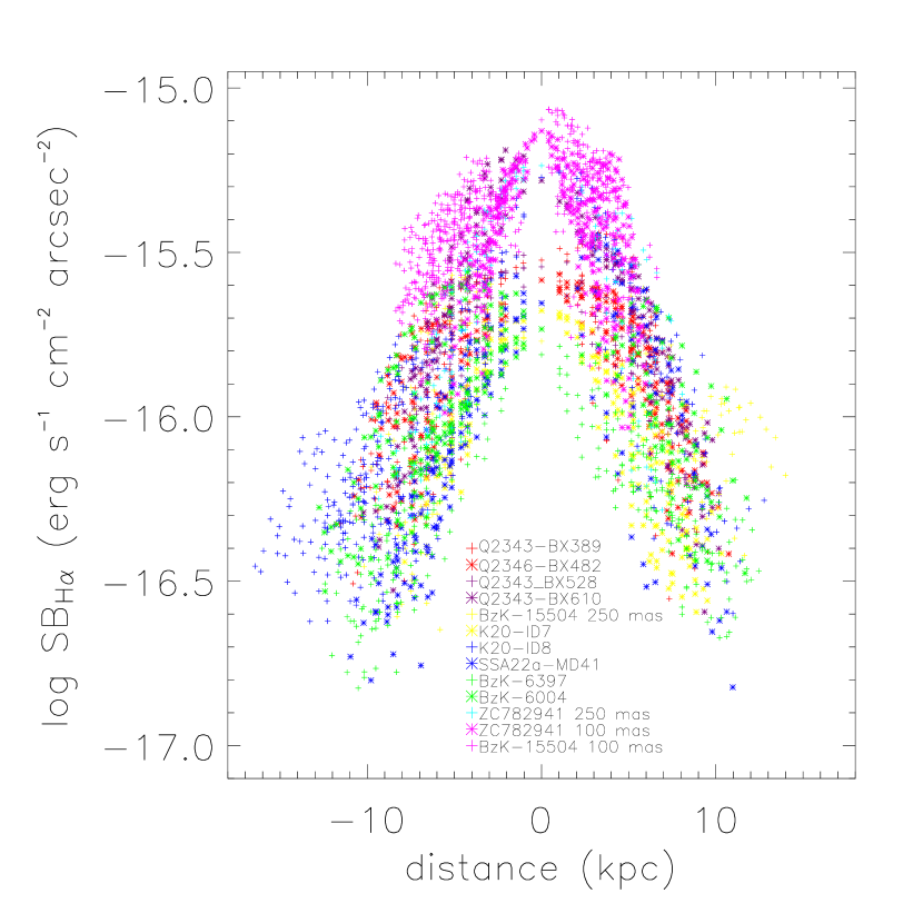
Figure 5.— A plot of the observed H$\alpha$ surface brightness versus the projected physical radius. The surface brightness has not been corrected for cosmological dimming. Each point represents a position centered on one pixel of $0^{\prime\prime}\,.\hskip 0.28453pt125$$\times$$0^{\prime\prime}\,.\hskip 0.28453pt125$ , whereas the data were smoothed by 3$\times$3 pixels, i.e., averaged in areas of size $0^{\prime\prime}\,.\hskip 0.28453pt375$$\times$$0^{\prime\prime}\,.\hskip 0.28453pt375$. As the spatial resolution is typically $\sim$ $0^{\prime\prime}\,.\hskip 0.28453pt5$-$0^{\prime\prime}\,.\hskip 0.28453pt6$ (or $\sim$4$-$5 pixels), the points are therefore not independent, and each data set has a limited number of independent points (about 5-10, see Shapiro et al., 2008). The legend to the figure indicates each galaxy in our sample. The zero radius was chosen to represent the symmetry point in either the kinematics or the outer isophotal H$\alpha$ distribution. The distribution of surface brightness is not symmetrical for most of the sources.

However, beam smearing is worrying in that the trends we observe will obviously be influenced by our poor resolution. We must take care in determining what the true impact of our poor resolution might actually be on the distribution and kinematics of the emission line gas. We observe the trends with H$\alpha$ surface brightness over physical scales that are $\sim$6$\times$ larger than the spatial resolution of our data. To investigate explicitly whether this may be an artifact due to low spatial resolution we constructed several simple models that have bright central point sources with broad lines. Such models would correspond to a bright AGN or concentration of mass increasing the velocity dispersion in the centers of these galaxies. Although this may appear unphysical, since we do not see bright point sources, it will help to investigate, for example, the effects of a narrow-line AGN. Our toy models (not shown) do not reproduce the observed trends, which implies it is very difficult to contrive a realistic situation where only the poor resolution of our data would lead to the trends we observe between surface brightness and radius.

Could beam smearing induce an apparent relationship between line width and surface brightness? Could this trend be related to distant galaxies having more complex light profiles? To understand the impact of beam smearing and complex light profiles of these galaxies on our analysis, we constructed simulated data cubes using the light distributions observed in NICMOS H-band images of five galaxies in our sample (Fig. 4). We assumed that the line emission follows the distribution of the H-band flux, that the velocity dispersion is 25 km s^-1 independent of position or radius (Epinat et al., 2009), and that the rotation curves and peak velocities are those from Förster Schreiber et al. (2006). We did not include noise in this display as it results in a scatter plot about the assumed constant velocity dispersion, masking the trend of some pixels to reach high dispersions (which we think is extremely important to make obvious). Thus for clarity, we do not show a plot of our analysis with noise.

As we can see in Fig. 8, assuming typical velocity dispersions seen in local disk galaxies and light distributions of distant galaxies and smoothing them to our resolutions does not reproduce the data (see also Wright et al., 2008; Genzel et al., 2008; Förster Schreiber et al., 2006). We do see that there are some regions of high dispersion, but this makes up a small number of pixels whereas a great majority of the regions, regardless of their relative surface brightness have dispersions similar to what we initially assumed (i.e., 25 km s^-1). This, coupled with the lack of increase in the dispersions when comparing our seeing limited data with that taken using adaptive optics, suggests that beam smearing, while obviously playing a role in these trends, does not cause these trends.

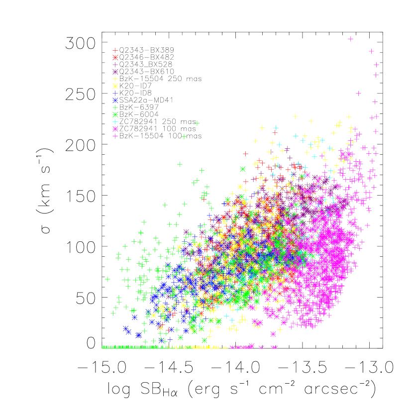
Figure 6.— Plot of the H$\alpha$ surface brightness (now corrected for surface brightness dimming) versus the observed velocity dispersion. See Fig. 5 for details on the 3$\times$3 pixel smoothing that was applied. The legend to the figure indicates which symbol represents which galaxy in our sample. There appears to be a relationship between surface brightness in H$\alpha$ and the line width for both the ensemble of sources as well as within individual sources. Because of the trend between surface brightness and dispersion, velocity dispersions below the resolution of our data, about 50 km s^-1 for the sources observed in the K-band (all but one of the sources shown here) and about 60 km s^-1 for BzK-6397 have particularly large relative uncertainties.

4. Emission-line properties of high-redshift galaxies

Given the high star-formation rates (Förster Schreiber et al., 2006; Genzel et al., 2008) and emission line surface brightnesses in these galaxies, we hypothesize that the high surface brightnesses and relationship between velocity dispersion and surface brightness in H$\alpha$, may be explained by postulating that the intense star formation is pressure-driven by mechanical energy input from the starburst itself and self-gravity of gas at high surface densities. In this sense, the star formation will be self-regulated. We will argue that these systems may be analogous to nearby starburst galaxies, such as M82, except that at high redshift, the intense star formation and strong mechanical energy injection must act over significantly larger areas (10-20 kpc compared to a few kpc, e.g., Heckman et al., 1990; Lehnert & Heckman, 1996a), but with a similar local surface brightness and similarly high pressures. However, this is not the only possibility and we will explicitly address different scenarios to investigate whether these relationship may be generated by cosmological gas accretion or gravitationally unstable disks. Some of our main arguments will rely on the detection of nebular emission lines like [NII]$\lambda$6583, [SII]$\lambda$$\lambda$6716,6731 or [OI]$\lambda$6300, which are relatively faint in high-redshift galaxies. We detected all of these lines in only one galaxy, while we detect all but [OI]$\lambda$6300 in 5 others. Where one of the lines is undetected or severely affected by a telluric night sky line, we give upper limits, provided that they are physically meaningful. For a subsample of 5 targets, our data include H$\beta$ and [OIII]$\lambda\lambda$4959,5007, which fall into the near-infrared H-band for redshifts z$>$2. These data sets have not been discussed previously in the literature. We list the integrated emission line properties of these galaxies in Table 1. As the H-band data are rather shallow relative to the K-band, we typically detect only the highest surface brightness regions (and likely also regions of relatively low extinction).

We extracted emission line ratios from matched apertures in the H and K band data sets, covering the areas where line emission is detected in the H band. We use the measured, and not the extinction corrected line fluxes for the emission line diagnostics. This adds only a minor uncertainty, given the relatively low signal-to-noise ratio of our data, low luminosities of the low-ionization lines, and the fact that we will only use ratios of lines with very similar rest-frame wavelengths.

4.1. Extinctions

We estimated extinctions for the four objects with measured H$\alpha$ and H$\beta$ fluxes (Table 2). H$\beta$ in Q2346-BX482, which would have been a fifth galaxy with a H$\beta$ flux and extinction estimate, and the emission in the north of Q2343-BX389 are severely affected by night sky lines (so the measurement is only for the southern part of the galaxy), and for three other galaxies we identified the areas with reasonably bright H$\beta$ emission, and extracted H$\alpha$ from the same aperture (Table 2). For a galactic extinction law, and an intrinsic Balmer ratio of F_Hα /F_Hβ $=$2.86, we find extinctions in the range of A${}_{V}\sim$ 1$-$2 magnitudes. This corresponds to correction factors of about 2$-$5 between observed and intrinsic H$\alpha$ luminosities. We will neglect extinction in much of our subsequent discussion, but caution that intrinsic values are strict lower limits and may have been underestimated by factors of a few.

4.2. Electron densities and pressures

The line ratio of the [Sii] doublet, [Sii]$\lambda$6716/[Sii]$\lambda$6731, is density-sensitive in the range of $\sim 10^{1-5}$ cm^-3. These lines are relatively faint, but we have robustly detected and spectrally resolved this doublet in six galaxies in our sample, at signal-to-noise ratios $\sim 10$. We are thus able to measure electron densities directly, and to estimate the pressure in the partially ionized zones within the interstellar medium. Densities listed in Table 3 are in the range $\sim$ 100$-$1000 cm^-3. Such values are typical, if not higher, than densities in the starburst regions of galaxies in the local Universe (such as M82; Lehnert & Heckman, 1996a) and suggest thermal pressures of about 10${}^{-8.5}-10^{-9.5}$ dyne cm^-2, i.e., several orders of magnitude higher than in the interstellar medium in normal nearby galaxies. Similar pressures are found for the z$=$2.6 submillimeter galaxy SMMJ14011+0252 (Nesvadba et al., 2007). We will argue below that the ambient medium of our galaxies is highly pressurized, and show that these estimates are also consistent with pressures derived directly from photoionization models.

The high pressures may also explain another remarkable feature of our galaxies, namely their overall low ratios of low-ionization lines like [Sii]$\lambda\lambda$6716,6731 and [Nii]$\lambda$6583 compared to the high H$\alpha$ luminosities. While the recombination lines increase linearly with increasing density and ionization parameter, the ratio of [Sii]$\lambda\lambda$6716,6731 will decline with increasing ionization parameter (e.g., Wang et al., 1999). Since the gas with the highest surface brightness also has a declining ratio, measuring the density from the [Sii] lines becomes more difficult as the surface brightness increases. Thus, it may not be surprising that we obtained [Sii] measurements at sufficiently high signal-to-noise only for parts of our sample. This may also affect other diagnostic line ratios. Larger samples of high-redshift galaxies with deep spectroscopy of a comprehensive set of faint, diagnostic lines will help to secure these findings.

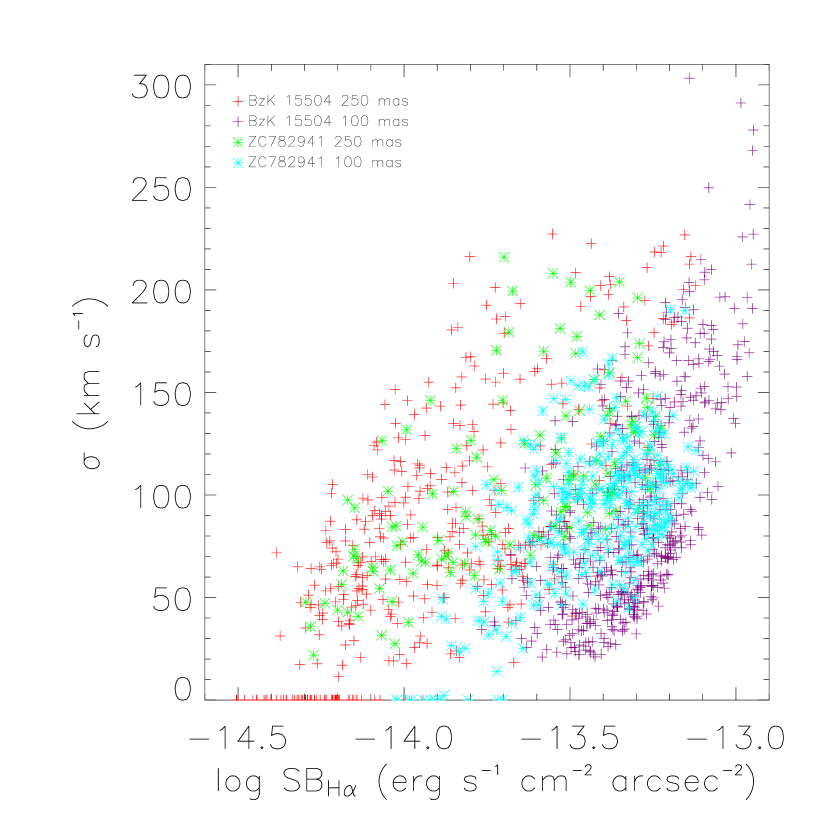
Figure 7.— Plot of the rest-frame H$\alpha$ surface brightness versus the observed velocity dispersion for the 2 galaxies for which we have both seeing limited and adaptive optics assisted data sets (ZC782941 and BzK-15504). Individual points in the data cubes were treated as shown in Fig. 6. In the case of the data cubes that were taken with adaptive optics assistance, the pixel scale is 50 mas pixel^-1 and they were also averaged over 3$\times$3 pixels (Fig. LABEL:fig:S_BHaradius. There is an increase in the velocity dispersion of some of the regions within BzK-15504 but these are entirely associated with the region of and around the AGN, substantiating our claim that BzK-15504 hosts an AGN (see also Genzel et al., 2006).

4.3. Diagnostic line ratios

Baldwin et al. (1981) and Veilleux & Osterbrock (1987) advocated the use of characteristic ratios of the bright optical nebular emission lines as diagnostics to differentiate between ionization due to starbursts and AGN. These so-called BPT diagrams relate the strengths of lines like [Nii]$\lambda$6583, [Oi]$\lambda$6300, or [Sii]$\lambda\lambda$6716,6731 with those of the Balmer recombination lines and [Oiii]$\lambda$5007, and gives us the ability to trace the physical conditions, namely temperature and ionization parameter, in the emission line gas. Due to the different ionizing spectra of starbursts and AGN, galaxies will fall into characteristic areas of the diagrams when their nebular emission is dominated by photoionization from young stars, or by an active nucleus.

We show the results in Fig. 9 and 10, together with the loci of other galaxies at similarly high redshifts taken from the literature. It should be noted that all of these diagnostics are to a large degree empirical and developed for galaxies at low redshift, and that different evolutionary stages may influence the emission line diagnostics in a rather subtle way. As already stated by Erb et al. (2006a), many z$\sim 2-3$ galaxies are shifted towards higher low-ionization line ratios relative to the low-redshift relationships. Brinchmann et al. (2008) argued by analogy with a subsample of local galaxies from the SDSS that this may be a result of higher pressures and higher ionization in high redshift galaxies.

However, this is not the only effect we may expect to take place. At low redshift, luminous AGNs reside predominantly in relatively massive galaxies which have comparably high ($\mathrel{\hbox{\hbox to0.0pt{\hbox{\lower 4.0pt\hbox{$\sim$}}\hss}\hbox{$>$}}}$solar) metallicities. At high redshift, this is not necessarily the case. Groves et al. (2006) modeled the expected position of AGN in low-metallicity host galaxies in classical emission line/ionization diagrams (e.g., [Nii]/H$\alpha$ versus [OIII]/H$\beta$). They find that the metallicity-sensitive [Nii]/H$\alpha$ ratio will be shifted towards lower values for AGN with low-metallicity narrow line regions. Seyfert galaxies and QSOs have ratios of [OIII]/H$\beta$ that are higher than those of HII regions and star-forming galaxies in such diagrams. Since the ratio of, for example, [OIII]/H$\beta$ is not strongly affected by lower the metallicity, the position of low-metallicity AGN in ionization diagrams may lie above the locus occupied by HII regions. We illustrate this effect by showing the position of the low-redshift, low-metallicity AGN of Groves et al. (2006) in the same diagram. Interestingly, most optically or UV-selected starbursts fall very close to the region spanned by the Groves et al. sample. This is not to say that these will be low-metallicity AGN, in particular, since the observed strong starbursts will create high-ionization, high-pressure environments, which will shift the galaxies towards the AGN part of the diagram (Brinchmann et al., 2008). However, this does imply that we may significantly underestimate the fraction of high-redshift galaxies with AGN of rather moderate luminosity. In the following we discuss the specific example of an obscured quasar with relatively inauspicious diagnostic line ratios compared to optically selected QSOs.

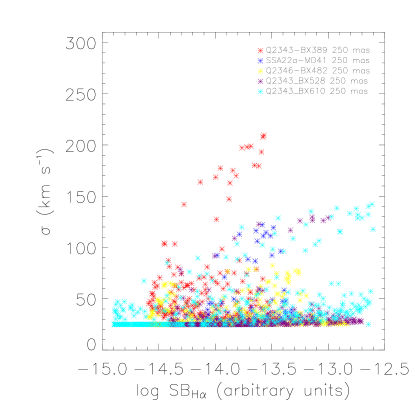
Figure 8.— A plot of surface brightness versus velocity dispersion for a set of toy models. Each of the “models” was generated assuming the distribution of light of the HST/NICMOS image, an intrinsic and uniform velocity dispersion of 25 km s^-1, a distribution of rotation velocity and a velocity peak as given in Förster Schreiber et al. (2006), and a point spread function with a FWHM of $0^{\prime\prime}\,.\hskip 0.28453pt6$. Care was taken to ensure that the final resolution of the data set was $0^{\prime\prime}\,.\hskip 0.28453pt6$ and took into account the intrinsic resolution of NICMOS. For the presentation here, we did not include noise as it would simply tend to increase the scatter, especially at the low surface brightnesses, but not change the overall trend that the dispersion would remain roughly constant.

5. The powerful Active Galactic Nucleus of BzK-15504

We will now give an example from among the galaxies of our sample, BzK-15504, where the AGN plays a role that is almost certainly non-negligible in interpreting the extended emission of the host galaxy. This galaxy falls within the range of low-metallicity AGN in the [Nii]/H$\alpha$ versus [Oiii]$/$H$\beta$ diagnostic diagram discussed by Groves et al. (2006), but also near the dividing line between AGN and starbursts. Thus, the impact of AGN photoionization will easily be missed with a diagnostic based only on local galaxies since powerful AGN embedded in low metallicity host galaxies are relatively rare (Groves et al., 2006). We use additional constraints, in particular the [Oi]/H$\alpha$ ratio and the near-nuclear [Oiii]$\lambda$5007 luminosity to argue that this galaxy hosts an obscured quasar, and that most of the extended H$\alpha$ emission may in fact be part of an AGN ionization cone. This calls into question previous interpretations of the star-formation properties and accretion rates in this galaxy (see also § 8.2). While this is the only clear case among the 11 galaxies discussed here, it does illustrate that the rest-frame optical emission line diagnostics for z$\sim 2$ galaxies, including the 11 discussed here, may be less straight-forward to interpret than previously realized.

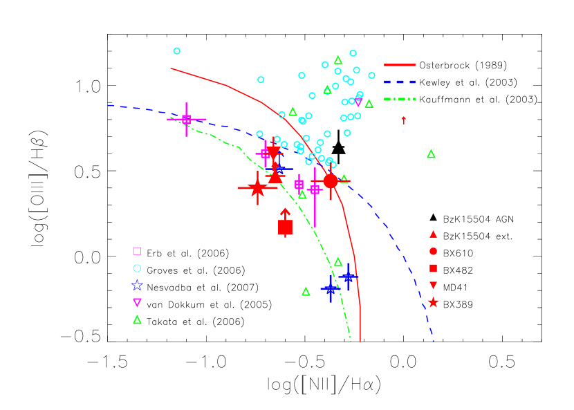
Figure 9.— The optical emission line ratios, [Nii]$\lambda$6583/H$\alpha$ versus [Oiii]$\lambda$5007/H$\beta$ for some of the galaxies in our sample (BzK-15504, BX610, BX482, MD41, and BX389), as well as for some distant and local galaxies taken from the literature (Erb et al., 2006a; Groves et al., 2006; Nesvadba et al., 2007; van Dokkum et al., 2005; Takata et al., 2006). The dividing lines within the diagram demarcate the separate regions occupied by galaxies whose emission lines are dominated by heating due to star formation from those dominated by active galactic nuclei (Kauffmann et al., 2003; Kewley et al., 2001; Osterbrock, 1989). Interestingly, many of the galaxies in this sample fall near the dividing line, which is consistent with either heating due to AGN, as is the case for both the nucleus and the extended emission line gas in BzK-15506.

5.1. The Bolometric Luminosity of the QSO in BzK-15504

It is clear that the nuclear emission lines of BzK-15504 lie within the region of the AGN in all of the emission line diagrams suggesting that it is indeed a powerful AGN (Fig. 9 and 10). The bolometric luminosity is an important parameter as it sets the total energy output of the AGN. BzK-15504 has not been observed over a sufficiently wide range of wavelengths to estimate its bolometric luminosity accurately. Heckman et al. (2004) argue that [Oiii]$\lambda$5007 luminosity can be used to estimate the bolometric luminosity of AGN over the range of L_[OIII]=10^6.5 to 10⁹ L_☉. Their adopted relationship is L_bol=3500L_[OIII] with a scatter of about a factor of 2 (see Heckman et al., 2004, and references therein for details). Using this relation for our [Oiii]$\lambda$5007 flux from BzK-15504 centered on the brightest continuum and line emitting region suggests that it has L_[OIII]=10^9.5 L_☉ and an implied L_bol=10^13.0 L_☉. Extinction correcting the [Oiii]$\lambda$5007 flux would increase it by 0.5 dex. BzK-15504 hosts a powerful AGN indeed – a QSO!

5.2. BzK-15504 as a giant Narrow Line Region?

In addition to the nuclear line ratios, the line ratios of the extended emission in BzK-15504 suggest that it could be photoionized by the AGN. In Fig. 9 and 10, we show the BPT diagrams for various line emitting regions within BzK-15504, and the line ratios lie either near the star formation-AGN boundary, as in the diagrams of [Oiii]/H$\beta$ versus [Sii]/H$\alpha$ and [Oiii]/H$\beta$ versus [Nii]/H$\alpha$, or clearly within the AGN region as in the [Oiii]/H$\beta$ versus [Oi]/H$\alpha$ diagram.

This of course is perhaps obvious from the fact that the surface brightness of the extended emission line region of BzK-15504 is very high, one of the highest in the sample (Fig. 5). However, can illumination by a central AGN explain the light profile of BzK-15504? The light profile of BzK-15504 has a ${{1}\over{r^{2}}}$ in its H$\alpha$ surface brightness dependence and is thus consistent with photoionization from a point source such as an AGN. However, since the emission is somewhat complex, this is not a strong constraint as other light profiles might equally well fit the data. Our point here is to suggest that it is at least “consistent” with a ${{1}\over{r^{2}}}$ profile. Making this assumption allows us to make a rough estimate of the ionization parameter,

$$\bar{\rm U}_{0}=S_{QSO}/c\bar{\rm n}_{H};\ \bar{\rm n}_{H}={{P_{gas}}\over{k10^{4}}}$$ (1)

where c is the speed of light, $S_{QSO}$ is the photon intensity at radius r from the QSO, and where we used, $L_{QSO}=10^{45.5}$ erg s^-1 (or 1/10 of the total bolometric luminosity), a radius of about 6 kpc, a rough density of 500 cm^-3 and a factor of 3 between the electron density and total density to reflect the fact that most of the [Sii]$\lambda\lambda$6716,6731 forms in the partially ionized zone. Using these numbers suggests that $\bar{\rm U}_{0}$ is about 10^-3. As we will see later, this is a rather canonical number for some of the other galaxies in the sample and not surprising given the surface brightness of all the galaxies.

Looking at this from another perspective, we can estimate that it takes a few percent of the total bolometric luminosity to explain the total H$\alpha$ emission in BzK-15504, if we make a simple recombination estimate for the number of ionizing photons. This is less than the 10% we assumed above, but overall consistent with the nebula being completely powered by the QSO. We note that this is obviously a lower limit as we have not considered the extinction in the extended nebular emission.

The total ionized gas mass is straight-forward to estimate as well. If we assume simple case B recombination as we did previously to estimate the total ionizing luminosity necessary to power the nebula, we find that we need about,

$${\rm M}_{H}={{{L_{H\alpha}}}\over{h\nu_{H\alpha}\alpha^{eff}_{H\alpha}}}m_{p}n_{e}^{-1}$$

$$=9.73\times 10^{8}L_{H\alpha,43}n_{e,100}^{-1}\ {\rm M}_{\sun}$$ (2)

Using $n_{e}$=500 cm^-3 and $L_{H\alpha,43}$=10^0.8, we find a total mass necessary to sustain the H$\alpha$ luminosity of about 3 $\times$ 10⁸ $M_{\sun}$. This is a rather modest amount of mass and shows that it is very simple to have the AGN ionize this much gas, which is only a small fraction of the total mass.

Given these estimates, we appear to be able to explain the emission line ratios with our estimated ionization parameter, looking at the emission line diagrams and physical parameters for photoionized nebulae in Groves et al. (2004, 2006). The line ratios are indeed consistent with having Hydrogen number densities of-order 100-1000 cm^-3 and a dilute ionizing energy field (log $\bar{\rm U}_{0}\sim-3$).

There are of course analogs to this situation in both the local and high redshift Universe. At high redshifts, optical emission line ionization cones over scales of kpc to 100 kpc are seen in powerful radio galaxies (e.g., Nesvadba et al., 2006b, 2008b). Emission line nebulae this large are generally seen in AGN with UV and emission line luminosities that are higher than observed for BzK-15504 (about a factor of a few to 10). However, the extended emission line region in BzK-15504 is consistent with luminosities observed in the “narrow line regions” of distant QSOs (Netzer et al., 2004).

AGN also show strong asymmetries in their emission line distributions. This may also explain the asymmetries seen in the emission line images of BzK-15504 (Genzel et al., 2006). It represents the asymmetry in the opening angle out of which the photons escape the AGN and where the gas falls within the beam. A local example of this is NGC 1068 (Veilleux et al., 2003). In NGC 1068, the circum-nuclear ionization cone shows a strong asymmetry in its distribution of [Oiii]$\lambda$5007 on both small scales (100s of parsecs; Evans et al., 1993) and large scale (kpc scales; Veilleux et al., 2003). Only in the areas of intense H$\alpha$ emission are the line ratios consistent with photoionization of massive stars in Hii regions. Over a much larger scale, 10s of kpc, in the areas of relatively low Hydrogen recombination line surface brightness are the line ratios consistent with photoionization by the AGN (Veilleux et al., 2003). Moreover, the emission line widths over the regions excited by the AGN (FWHM$\sim$100-few 100 km s^-1) are also in reasonable agreement with what is observed for BzK-15504. In many optically selected AGN, the line widths are not strongly influenced by the AGN despite the fact that the ionization state of the gas is (Nelson & Whittle, 1996). Of course, both the gas mass and the power of the AGN are larger in BzK-15504 and it may well be that as a result, the AGN can even outshine any star formation in the extended optical emission line emitting gas (Fig. 9 and 10). Within this regard it is also important to note that BzK-15504 also has one of the highest H$\alpha$ surface brightnesses in our sample. The AGN could be responsible for increasing its overall surface brightness as well as its AGN-like extended line emission. And like many classes of AGN (and in analogy with NGC1068 as just discussed) the radiation, although likely heavily attenuated, is able to escape to large distances despite the ionized gas representing a small fraction of the total gas mass of BzK-15504.

This last point is important. AGN host galaxies show a reasonable correlation between the size of their narrow line region and the luminosity in H$\beta$ (Bennert et al., 2002, but see, Netzer et al. 2004). The H$\beta$ luminosity of BzK-15504 would suggest a narrow line region size of a few to 10 kpc (this is without extinction correction). Interestingly, this is approximately the size of the emission line nebulae observed in H$\alpha$ and [OIII]. Thus, in agreement with other arguments, there is evidence that the extended emission line region is nothing more than a narrow line region around a powerful QSO with line widths that are, by analogy with local AGN, influenced, perhaps dominated, by other processes.

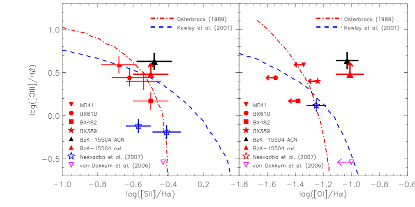
Figure 10.— The optical emission line ratios, [Sii]$\lambda\lambda$6716,6731/H$\alpha$ versus [Oiii]$\lambda$5007/H$\beta$ (left), and [Oi]$\lambda$6300/H$\alpha$ versus [Oiii]$\lambda$5007/H$\beta$ (right) for the same subsample as in Fig. 9. Again, the lines demarcate the regions of the emission line diagrams where the photoionization is dominated by star formation or AGN(Kewley et al., 2001; Osterbrock, 1989). These diagrams again demonstrate the role of the AGN in photoionizing BzK-15504. The other galaxies in the sample lie close to the lines of demarcation in the [Sii]$\lambda\lambda$6716,6731/H$\alpha$ versus [Oiii]$\lambda$5007/H$\beta$ diagram, but have limits that are consistent with being photoionized mainly by massive stars.

6. Nature of the emission line gas in these galaxies

The surface brightness in our sample is both very high, and a function of radius, velocity dispersion, and low ionization line emission ratio (i.e., [Nii]/H$\alpha$). This is in sharp contrast to what is observed for spiral galaxies in the local Universe where the velocity dispersion is roughly constant as the surface brightness declines exponentially. With the local trends in mind, we hypothesize that the trends seen in the distant galaxy data can be explained by self-regulated star formation whereby the intense star formation is pressure driven by the gas motions induced by the star formation itself. We attempt to show that essentially, these systems are analogous to the nearby starburst galaxies, such as M82 (and regulated perhaps in the same way as the ISM of the Milky Way) with an overall similar surface brightness and similarly high pressure, but with their star formation occurring over a much larger area.

6.1. The relation between H$\alpha$ surface brightness and [Nii]/H$\alpha$

In Fig. 11, we show the relationship between the emission line ratio [Nii]/H$\alpha$ and the surface brightness of H$\alpha$. An obvious way to understand such a relationship, in addition to the high H$\alpha$ intensity, is through the gas pressure in the cloud or cloud interfaces that gives rise to the recombination line emission.

To test this hypothesis we ran some simple photoionization models using the code Cloudy. The input spectrum was generated using Starburst99 (Leitherer et al., 1999) for a constant star formation rate and an age of 10⁸ years (consistent with the estimated ages of galaxies at z$\approx$2 Erb et al., 2006b). However, the exact age is not very important as long as it is sufficiently long for the spectral energy distribution, especially in the UV, to reach an equilibrium shape. It is thus appropriate for ages greater than about a few 10s Myrs and constant star-formation rate. We assumed a constant density slab with ionization parameters ranging from about log U=$-$5 to $-$1, initial densities log n=1, 2, and 3, and ISM metallicities and grain depletion which are kept constant for all calculations. These attempts at modeling are not intended to be exhaustive but illustrative. To gauge the impact of the ionization of the modeled cloud, we ran these calculations for two total column densities, 10²⁰ and 10²¹ cm^-2. The results from this modeling are shown together with the data in Fig. 11.

We can see that the range of [Nii]/H$\alpha$ and surface brightness can be explained by a combination of column density, volume densities, and moderately diffuse radiation fields. Obviously, such simple assumptions are not going to “fit” the data in any sense of the word, but show that the area of line ratio-surface brightness space covered by the data can be explained by a combination of these parameters, with each galaxy exhibiting some range in each of these. Surface brightness is linearly proportional to the density and ionization parameter, while the line ratio depends on roughly one over the square root of the ionization parameter for the range of ionization necessary to explain the line ratios. Such a high density and ionization rate implies that the ISM of these galaxies must in general exhibit high thermal pressures, P/k$\sim$10^6-7 K cm^-3 or more. The true maximum pressures are likely to be higher as our physical resolution is only about a few kpc making it difficult to identify the regions of highest surface brightness.

These pressures are much higher than observed in the disk of our Milky Way or other nearby normal galaxies. As discussed in Blitz & Rosolowsky (2006), and references therein, the hydrostatic mid-plane pressure in the MW is about 10^3.3-4.3 cm^-3 K, while for other local spirals it can range up to about 10⁶ cm^-3 K but is typically about 10^4.6 cm^-3 K. There have been fewer estimates of the more appropriate comparison, namely the thermal pressures. In the nuclear regions of local starburst galaxies, the thermal pressures as estimated from the ratio [Sii]$\lambda$6716/[Sii]$\lambda$6731 give values that range from 10^-9.3 to 10^-8.5 dyne cm^-2 or typically about 10⁷ cm^-3 K (Lehnert & Heckman, 1996a) similar to that observed here at z$\sim$2. Interestingly, Brinchmann et al. (2008) make a similar argument for galaxies that generally fall off the locus of the Hii regions in the [Oiii]/H$\beta$ versus [Nii]/H$\alpha$ diagram and lie close to the dividing line between Hii region and AGN excitation. They find that such galaxies have high specific star-formation rates, as do the general population of high redshift galaxies discussed here, and relatively large H$\alpha$ equivalent widths. Brinchmann et al. suggest that the most likely explanation for this is higher density (pressure) and that the escape fraction may be higher in the star-forming regions implying that the nebulae are at least partially density bounded. Similarly, in Fig. 11 we see that the clouds with column densities of log N_H=20 become density bounded at high ionization parameters and may explain the surface brightness limits we observe. Thus the pressures estimated from the photoionization models are consistent with those of nearby actively star-forming galaxies (Heckman et al., 1990; Wang et al., 1999).

6.2. Consistency with high ionization lines

In addition, for some of the galaxies we have H-band data cubes of sufficient signal-to-noise to investigate the ratio of [Oiii]$\lambda$5007 and H$\beta$. The photoionization models would predict [Oiii]$\lambda$5007/H$\beta$ of about 0.5-2.0. Indeed, not considering BzK-15504, which is powered by a QSO, the other galaxies show ratios consistent with the high ionization line ratios and again amplifying the idea that these nebula have increased density compared to nearby galaxies as observed by Brinchmann et al. (2008).

7. Powering the local motions in these galaxies

We have argued that the ISM of these distant galaxies is under high pressure and that this high pressure could be induced by the intense star formation within these systems. Fundamentally, this argument is analogous to the situation in the most intense starbursts in the local Universe such as M82 (e.g., Heckman et al., 1990; Lehnert & Heckman, 1996a; Lehnert et al., 1999). Such a hypothesis nicely explains some of the unusual features in these distant star-forming galaxies such as their high surface brightnesses in the recombination line(s) (which makes them observable in the first place), the low ionization line ratios, the ratio of the [Sii] lines (suggestive of high densities), and the trend for more intense star formation to lead to broader lines. We observe low ratios ($\sim$2-4) of v/$\sigma$ in the extended line emitting regions of our objects, much lower than the ratio of $\sim$10 generally observed in local and intermediate redshift disk galaxies, and this appears to be driven mainly by unusually high velocity dispersions, not low velocity shears.

In principle, the high velocity dispersions observed in the ionized gas lines are likely not representative of the turbulence in the whole star-forming ISM. Nevertheless, the energy injection necessary to sustain the high velocity dispersions observed in the ionized gas should affect the atomic and molecular phases (although if it is a turbulent cascade, with energy injection on large scales, the velocity dispersion will likely be lower in denser gas but the $\rho\sigma^{2}$ will be the same; Joung, Mac Low, & Bryan, 2008). Indeed, high dispersions in the gas out of which stars form is suggested by the large sizes and masses of high-redshift star-forming regions (giant clumps equaling the Jeans mass, Elmegreen & Elmegreen, 2005). This is also supported by the thickness of high-redshift disks when observed edge-on (Elmegreen & Elmegreen, 2006).

What is the power source of the high velocity dispersions that are observed, and that should affect the whole ISM of high-redshift galaxies? There are several possible mechanisms: (1) the conversion of potential energy of infalling material in turbulent gas which has sufficient angular momentum to relax into a disk configuration (cosmological accretion; Förster Schreiber et al., 2006; Dekel et al., 2009b); (2) peculiar motions in unstable disks that lead to perturbations in the velocity fields that are not resolved in our data and lead to a high $\sigma$ without consisting of real small-scale turbulence (e.g., Bournaud et al., 2008); (3) self-gravitationally generated turbulence (Wada et al., 2002); and/or (4) the combined effect of the intense star formation.

To characterize the order-of-magnitude needed to power the turbulence, we shall start by estimating its energy budget (if that is what these motions represent). Our low spatial resolution in the rest-frame of the galaxies does not allow us to cleanly separate these possible sources of the observed broad line emission. In fact, Mac Low (1999) as well as our astrophysical reasoning below imply that bulk motion and turbulence are intricately related in some of the scenarios, in the sense that bulk motion will inject kinetic energy into the system which will then be dissipated through turbulence. However, carefully examining the total energy contained within the emission line gas may help us constrain the mechanism responsible for its characteristics. We first consider the energy dissipated within the turbulence and whether or not it is consistent with cosmological accretion of gas.

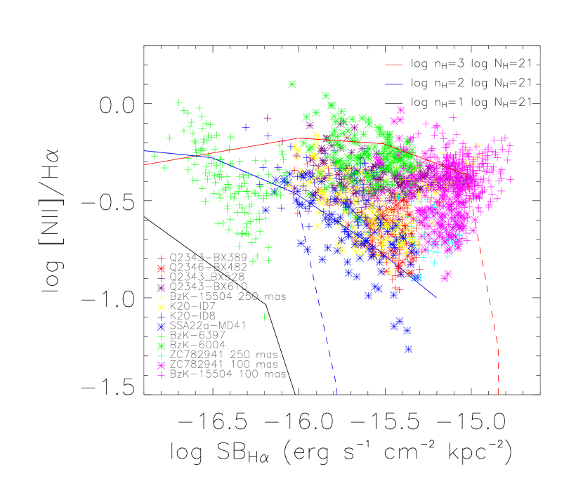
Figure 11.— The H$\alpha$ surface brightness (corrected for surface brightness dimming) versus the logarithm of the [Nii]$\lambda$6583/H$\alpha$ line ratio for all the individual spectra of the galaxies in our sample. The galaxies are labeled in the legend to the figure. The lines represent results for photoionization modeling (see text for details) for 6 set of conditions. The lines represent a range of density (log n_H=1 to 3) and column densities of log N_H=21 cm^-2 (solid lines) and log N_H=20 cm^-2 (dotted lines). The ionization parameters span from log U=$-$5 to $-$1.0 (which increases from left to right along the lines, meaning low ionization parameters have relatively high log [Nii]/H$\alpha$ and low H$\alpha$ surface brightnesses).

7.1. Turbulent energy dissipation

The violent motions observed in these distant galaxies are highly supersonic given the densities derived previously for the optical emission line gas and the turbulence generated, compressible. To estimate the dissipation of the turbulent energy therefore requires comparison with (magneto-)hydrodynamic simulations of a realistic interstellar medium. Mac Low (1999) provides an estimate of the energy dissipation rate for compressible turbulence as,

$$\dot{\rm E}_{kin}\simeq-n_{\nu}m\tilde{k}v_{rms}^{3}$$

where $n_{\nu}$ is a constant of proportionality, which Mac Low (1999) estimates to be 0.21/$\pi$, $v_{rms}$ is the root mean square of the velocity in the region, $m$ is the total mass, $E_{kin}$ is the kinetic energy, and $\tilde{k}$ is the driving wavenumber. Although, the validity of this energy dissipation estimate on galaxy scales has yet to be verified, it is useful to give an order-of-magnitude estimate of the energy injection rate necessary to sustain the motions we observe.

The parameters necessary to estimate the energy dissipation rate of compressible turbulence span a wide range of values. For example, the velocity dispersions observed in the galaxies range from about $<$40 km s^-1, in the outer regions, to about 250 km s^-1 in the inner, circum-nuclear regions (Fig. 6). The typical velocity dispersion is of-order $\sim$100-150 km s^-1. The driving scale is particularly difficult to estimate since the driving mechanisms likely operate over a wide range of scales (e.g., Joung, Mac Low, & Bryan, 2008). For example, if the largest scale driving mechanism was the cosmological accretion of gas, we would expect this scale to be large (Dekel et al., 2009b) approximately that of the thickness of the disk. Alternatively, if the driving mechanism is star-formation, the size of the largest star-forming regions or associations in the galaxies might be the appropriate scale. The clumps seen in Fig. 4 are approximately 100s of parsecs to kpc in diameter. Since the driving wavenumber is inversely proportional to the driving length, assuming a small scale for the driving length would tend to increase the energy dissipated through turbulence.

We cannot estimate the total mass of gas in the galaxies in a straight forward way. For simplicity, we will apply the Schmidt-Kennicutt law (Kennicutt, 1998a) to the star-formation intensities estimated from the H$\alpha$ surface brightness distribution. This relation implies that the gas surface densities are of-order $\Sigma_{gas}=10^{2.6}{\rm M}_{\sun}{\rm pc}^{-2}$ for star-formation intensities of 1 M_☉ yr^-1 kpc^-2 (1 M_☉ yr^-1 kpc^-2 is the typical average value for the star-formation intensity approximately averaged over the isophotal radius). This of course assumes that the molecular gas has same kinematics as the warm ionized gas. The high densities that we found in § 6.1 and the course angular resolution of our data which averages the kinematics over a large region perhaps imply that this is not a bad assumption (but see Joung, Mac Low, & Bryan, 2008; Walter et al., 2002).

If we adopt, $v_{rms}$=150 km s^-1, a mass surface density of 1000 M_☉ pc^-2, a driving length of 1 kpc (which is a typical thickness of the “clumpy disks” observed at similar redshifts as our sample; Elmegreen & Elmegreen, 2006), we find that turbulence likely dissipates about 10⁴² erg s^-1 kpc^-2. The surface area within the isophotal radius is approximately 200 kpc² (Table 1) giving a total energy dissipation of about 10^44.3 erg s^-1. We emphasize given the uncertainties, the limits of our theoretical understanding of turbulence and untested assumptions, this estimate of the turbulent dissipation should be considered as order-of-magnitude only.

7.2. Cosmological gas accretion

We can compare this rough energy dissipation estimate with that of gas infalling on to the disk itself. The total energy accretion rate from gas falling onto the disk is given approximately by (Dekel & Birnboim, 2008),

$$\dot{\rm E}_{heating}=\mid\Delta\phi\mid\dot{M}_{gas}=4.8\dot{M}_{gas}V_{c}^{2}$$

$$=10^{43.1}\dot{M}_{gas,100}V_{c,200}^{2}\ {\rm erg}\ {\rm s}^{-1}$$ (3)

where $\mid\Delta\phi\mid$ is the potential energy of infall, $\dot{M}_{gas,100}$ is the halo gas accretion rate in units of 100 M_☉ yr^-1 and $V_{c,200}$ is the circular velocity of the halo in units of 200 km s^-1. Thus it appears that accretion of gas in itself cannot power the turbulent and bulk motions we observe in these galaxies if these motions decay as compressable turbulence. Dekel et al. (2009a) also suggest that the main source of turbulence is not infalling gas, unless this infalling gas is itself also highly clumpy, something they themselves rule out as highly unlikely for a large fraction of the infalling gas.

7.3. Velocity dispersions in Jeans unstable clumps

The dynamics of these galaxies could be influenced by the mode of star formation. Elmegreen and collaborators have proposed that the large number of clump-cluster and chain galaxies observed at high resolution in deep HST imagery represent gas-rich Jeans unstable disks (review in Elmegreen, 2007). Clumpy galaxies are not rare. Their frequency and relatively fast dynamical evolution suggests that perhaps all galaxies pass through a “clumpy” stage in their evolution and that this process is a natural way of explaining phenomena like the growth of bulges and nuclear supermassive black holes (Bournaud et al., 2007; Elmegreen et al., 2008a). HST/NICMOS images of five of our sample galaxies (Fig. 4) do show that they have “clumpy” irregular morphologies consistent with this hypothesis.

The clumpiness of the disks is hypothesized to be driven by Jeans instability, which implies a relationship between the mass of collapsing gas and the velocity dispersion within the gas (e.g., Elmegreen et al., 2007). Specifically, the Jeans relationship implies that,

$$\sigma_{gas}\sim M_{J}^{1/4}G^{1/2}\Sigma_{gas}^{1/4}=54M_{J,9}^{1/4}\Sigma_{SFR}^{0.18}\ {\rm km}\ {\rm s}^{-1}$$ (4)

where $\sigma_{gas}$ is the velocity dispersion of the gas, G is the gravitational constant, $\Sigma_{gas}$ is the gas surface density in M_☉ pc^-2, $M_{J,9}$ is the Jeans mass in units of 10⁹ M_☉, and $\Sigma_{SFR}$ is the star-formation intensity in units of M_☉ yr^-1 kpc^-2. We have used the Schmidt-Kennicutt relation (Kennicutt, 1998b) to convert from gas surface density to star-formation intensity. We show the relationship between the velocity dispersion and star-formation intensity for Jeans unstable clumps in Fig. 12 for a clump of 10⁹ M_☉, similar to the largest masses estimated for clumps based on spectral energy distribution fitting (Elmegreen & Elmegreen, 2005). We chose 10⁹ M_☉ to put the weakest limit on the possible contribution of the clumps to the observed velocity dispersion.

The velocity dispersions predicted by Eq. (6) generally lie below the data in Fig. 12, especially at the highest intensities, and the relationship is also too flat as a function of star-formation intensity. Although this does not rule out clumps in a disk as a contributing source to the high velocity dispersions observed in our sample, especially for the gas with lowest dispersions, it cannot be the entire explanation. And taken at face value, the masses necessary to explain the average dispersion would be more like 10¹⁰ M_☉, not 10⁹ M_☉ suggesting that the dispersions are not dominated by the internal dispersions of the clumps themselves.

7.4. Gravity powering turbulence in dense gas-rich galaxies

The clumpy light distributions observed suggest, in particular, that the clumps themselves may have required an earlier source of turbulence. This is necessary to ensure that the initial Jeans mass is as high as the clumps masses observed (up to more than $10^{9}M_{\sun}$; Elmegreen et al., 2007). This implies that we may be obliged to hypothesize another source of turbulence, especially in initiating the intense star formation, to favor and encourage the growth of massive clumps. Perhaps self-gravity powering the initial turbulence would play the necessary role (see Thomasson et al., 1991; Wada et al., 2002).

A gas disk with a low turbulent speed $\sigma$ may likely have a Toomre parameter $Q=\frac{\sigma\kappa}{\pi G\Sigma}<1$, if the surface density $\Sigma$ is high. As a result, gravitational instabilities will form and heat the gaseous medium, increasing its turbulent energy until Q reaches $\sim 1$ and the process stops. The observation of clumps in our z$\sim$2 galaxies and others suggest that Q is close to one, so that this is the level at which gravity could indeed power the turbulence. In local flocculent spiral galaxies, Elmegreen et al. (2003) argued that gravity was triggering the turbulence through local instabilities.

The hydrodynamic simulations by Agertz et al. (2009) have shown that disk self-gravity likely triggers the 5-10 km s^-1 turbulent speed of extended HI disks around local spirals – which could not result from star formation beyond the edge of star-forming disks (see also Wada et al., 2002). The density of these modeled disks is nevertheless far lower than the estimated density of gas disks at z$\sim$2. A gas fraction of $\sim$50% in these disks (from Daddi et al., 2008, observations or inferred from the Schmidt law, Bouché et al. 2007) indeed corresponds to typical gas surface densities of $\sim$500 M_☉ pc^-2. More direct hints on the role of self-gravity in high-redshift disks can be found in the models by Tasker & Bryan (2006, 2008), where gas disks with large-scale densities around 100 M_☉ pc^-2 are modeled, much closer to the hypothesized density at z$\sim$2 even if still somewhat lower. Interestingly, these models show larger clumps when the gas density is large, indicating larger Jeans masses and hence larger velocity dispersions. This is found in models of isolated disks without feedback, where only gravity can power turbulence. The addition of feedback from star-formation in these models does not change significantly the clump masses, hence the turbulent speed, suggesting that the early stages of turbulence development could be mostly powered by self-gravity. Direct models of disks at z$\sim$2 with high density would be desirable, but given that Tasker & Bryan (2008) have both the gas density and the clump masses/sizes somewhat lower than z$\sim$2 standards, it is reasonable to infer that disk self-gravity is likely important source of turbulence at high redshift but does not likely generate the extreme dispersions we observe (Fig. 12). As we noted earlier, it may be that the formation of massive clumps themselves requires high turbulence initially (Eqn. 5).

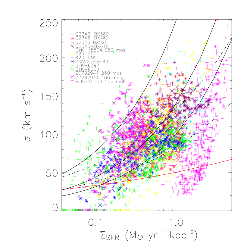
Figure 12.— A plot of the star-formation intensity versus the H$\alpha$ velocity dispersion in our sample of galaxies. See Fig. 1 for details on the 3$\times$3 pixel smoothing that was applied. The symbols for the different galaxies in our sample are shown in the legend to the figure. The solid black lines show three simple relationship of the form $\sigma=\surd{\epsilon\dot{E}}$, where $\epsilon$ is the efficiency of coupling between the energy injected and the ISM. (from bottom to top): $\sigma=100\surd\Sigma_{SFR}$ km s^-1, $\sigma=140\surd\Sigma_{SFR}$ km s^-1, and $\sigma=240\surd\Sigma_{SFR}$ km s^-1 (see text for further details). We note that the overall trend seen in the diagram for the ensemble of galaxies is also traced by the data from individual galaxies but with a somewhat steeper slope. If the dispersions represented turbulent motions, we would expect a scaling, $\sigma=(\epsilon\dot{E})^{1/3}$. Using two scalings for the coupling efficiency, 25% and 100% and a primary injection scale of 1 kpc, we find $\sigma=80\Sigma_{SFR}^{1/3}$ km s^-1 and $\sigma=130\Sigma_{SFR}^{1/3}$ km s^-1 (bottom and top black dashed curves respectively). The red solid line represents the velocity dispersion of a 10⁹ M_☉ clump using the simple Jeans relationship between mass and velocity dispersion (see text for details). The offset between galaxies may be due to a range of coupling efficiencies between the mechanical energy output from the on-going star formation, differences in the average pressure within the ISM, or geometrical factors such as inclination.

In addition, high velocity dispersions could be a result of mergers. In the local Universe, intensely star-forming galaxies show very high velocity dispersions in their optical emission line gas, up to 200 km s^-1 (Monreal-Ibero, Arribas, & Colina, 2006). To explain the low v/$\sigma$ observed at high redshift (Förster Schreiber et al., 2006), Robertson & Bullock (2008) proposed that a disk settling after a major gas-rich merger would have low v/$\sigma$. In particular, they construct their model to match approximately the properties of BzK-15504 in detail including its high star-formation rate and intensity (without the AGN). Thus, it is not clear how much of the dispersion is due to the intense star-formation and how much is driven purely by gravity in their model. Moreover, recently Bournaud & Elmegreen (2009) have criticised the merger model in that it does not naturally produce the clumpy morphologies that are frequently observed in distant galaxies and would lead to disks that make up a rather small fraction of the total mass. Thus it is not clear if gravitationally driven flows within mergers can produce the dispersions and high emission line surface brightness we observe without the accompanying intense star formation.

7.5. H$\alpha$ surface brightness–velocity dispersion: Powering the kinematics through star formation

We argued above that self-gravity may be an important source of turbulence at high redshift, but does not seem sufficient to generate the observed velocity dispersions (see also Fig. 12). This and the relationship between H$\alpha$ surface brightness and velocity dispersion suggests that the star formation within the galaxies is powering the dynamics of the emission line gas. If the star formation is indeed inducing the high pressures, then this is what would be expected. On purely dimensional grounds, if the energy output from young stars is controlling the dynamics of the emission line gas, we would expect, that $\sigma$, the velocity dispersion, would be proportional to the square root of the energy injection rate, dE_SF/dt, due to stars. If the coupling efficiency of the mechanical energy output of the star formation does not depend on radius, then the energy injection rate is simply proportional to the star-formation rate. In this case of course, the energy injection per unit area is proportional to the star-formation intensity. This hypothesis is equivalent to conserving (with some efficiency) the mechanical energy output of the star-formation within the ISM of the galaxy and that the velocities of the warm ionized gas trace this energy injection rate.

In Fig. 12, we have over-plotted just such a relationship. This is not a fit to the data, but a simple scaling law based on the star-formation rate per unit area and the velocity dispersion in the warm neutral/ionized gas in the disk of the MW and other nearby galaxies. The function is of the form, $\sigma$=($\epsilon\Sigma_{SFR}$)^1/2 where $\epsilon$ has been determined for the MW and other nearby galaxies where the velocity dispersion in H$\alpha$ and star-formation intensities have been related (see Dib et al., 2006, for details). There are several possible values for $\epsilon$ in this relationship. If we take a simple scaling from galaxies like the MW, they typically have star-formation intensities in the regime of $\Sigma_{SFR}$=10^-5 to 10^-3 M_☉ yr^-1 kpc^-2 and velocity dispersions in the warm ionized gas of-order 10 km s^-1. Dib et al. suggested that galaxies may change from a quiescent disk mode to a starburst mode at $\Sigma_{SFR}$=10^-2.5 to 10^-2 M_☉ yr^-1 kpc^-2. This comes from modeling the ISM with a coupling efficiency of 25% to the supernova energy from disk star formation. Using these two values for the scaling relation yields the bottom two curves in Fig. 12, whereas a coupling efficiency of 100% would yield the curve at the top in Fig. 12. We emphasize that the axis of abscissa is a simple scaling between H$\alpha$ surface brightness and the star-formation rate which was made assuming a relationship between star-formation rate and H$\alpha$ luminosity (Kennicutt, 1998a). We have not taken into account the effect of extinction in making this scaling. If the galaxies for which we have H$\beta$ measurements for are representative of our entire sample. This would increase the star-formation intensities by a factor of a few (Table 2).

While such a toy model is not a particularly good fit, especially at the highest star-formation intensities, it has the virtue of having no free parameters. It is just a simple scaling based on the MW and other nearby galaxies. Although we put this in context of the modeling done by Dib et al. (2006), we could as well have simply used the MW scaling of star-formation intensity and velocity dispersion. Obviously, the true nature of the interstellar media of these distant galaxies cannot be so simple as the energy injection argument presented here. This argument simply shows that the star formation in the galaxies themselves is likely controlling the dynamics of the emission line gas.

7.5.1 Mechanical energy due to star formation

Given the relationship between star formation intensity and the velocity dispersion of the gas, it is logical to investigate whether the star formation has sufficient global energy injection rates to drive the high velocity dispersions – much like our previous estimate in § 7.1 comparing the accretion energy rate from infalling cosmological gas. Using the relationship from Kennicutt (1998b) between H$\alpha$ luminosity and star-formation rate, we find that the total star-formation rate per unit area – the star-formation intensity – ranges from about 0.05-5 M_☉ yr^-1 kpc^-2 (Fig. 6). The dynamical time and integrated H$\alpha$ equivalent width of our sample of galaxies and that from the Erb et al. (2006b) sample, suggests that they may have been forming stars continuously at the observed rate for the last few $\times$ 10⁸ years. This implies that the ongoing star formation in this sample in total produces more than 10^41-42.5 erg s^-1 kpc^-2 of mechanical energy (Leitherer et al., 1999) for the range of large scale star-formation intensities observed. These numbers are lower limits since we do not have sufficient data to constrain the spatially resolved extinction and so the true star-formation intensities are likely to be higher (Table 2).

We can now compare this total energy injection rate with the value estimated § 7.1, namely 10^44.3 erg s^-1. For a fiducial value of 1 M_☉ yr^-1 kpc^-2, which is typical within a isophotal radius (Fig. 6), and the mechanical energy output rate given above, would suggest total energy injection rates of $>$10^44.2 erg s^-1. Since the numbers are similar, we suggest that the star-formation is powerful enough to maintain the turbulent and bulk motions observed.

7.5.2 Accelerating the emission line clouds

Having now argued that the star formation is injecting energy into the ISM of these galaxies and is sufficient to explain the overall dynamics of the gas and to support dissipation through turbulence, can we make a plausible model for how the clouds might be accelerated? Klein et al. (1994) and Nakamura et al. (2006) have developed both analytic models and simulations for clouds accelerated in a blast wave. Such a blast wave is expected to be generated by the intense star formation observed in our sample of galaxies. As the blast wave passes it shock heats the cloud and eventually destroys it through Kelvin-Helmholtz and Rayleigh-Taylor instabilities.

In this scenario, the turbulence is driven by large scale bulk motions induced by energy injection – blast waves generated by intense star-formation and other processes – over a wide range of scales, which then cascades into the denser gas and redistributes the energy over all scales in the medium finally dissipating mainly on the smallest scales (Joung, Mac Low, & Bryan, 2008; Mac Low & Klessen, 2004, and references therein). The nature of turbulence emphasizes the importance of both bulk and random motions and estimating energy dissipation rates based on turbulence arguments while estimating velocities based on bulk motion arguments are thus appropriate.

Klein et al. (1994) have found relatively simple analytic approximations that can capture the destruction time of clouds with a range of properties like contrast with the inter-cloud material, Mach number of the blast wave, etc. Although there is a problem with simply using these formulae with the parameters from the photoionization calculations because those are aimed at providing the emission lines without consideration of the shock heating in the first place, we envision a scenario where shock heating, despite the intense energy input from the supernova and stellar winds, is only a small fraction of the total energy output of the star formation. For our zeroth order model of star formation proceeding for 10⁸ years, we find that this condition is clearly satisfied (Leitherer et al., 1999). Thus we expect the emission lines to be dominated by the ionizing energy output from massive stars and not by the shock heating. The clouds could therefore be thought of as the ones that have yet to be destroyed or are simply the surfaces of sheets and filaments that will get eventually or are now being run over by the blast waves into the ISM.

The relationship for the acceleration of the cloud is given by Klein et al. (1994, but see also ), as,

$${\rm m_{c}}{{dv_{c}}\over{dt}}=-1/2{\rm C_{D}}\rho_{i,1}\acute{v}_{c}^{2}A$$ (5)

where, ${\rm m_{c}}$ is the mass of the cloud, ${{dv_{c}}\over{dt}}$ is the acceleration of the cloud, ${\rm C_{D}}\sim 1$ is the drag coefficient, $\rho_{i,1}$ is the post-shock density and is approximately, $\rho_{i,1}\simeq 4\rho_{i,0}$ (we are assuming strong shocks), the pre-shock density of the inter-cloud medium, and $\acute{v}_{c}=\mid v_{i,1}-v_{c}\mid$ is the relative velocity of the shocked medium, where $v_{i,1}$ is the mean velocity of the cloud, and $A$ is the cross-sectional area.

Does the star formation actually generate blast waves of sufficient energy to accelerate the clouds to the observed velocities? The total mass ejected by supernovae and stellar winds in the star formation process, $\dot{M}_{SF}$ can be scaled as $\dot{M}=\beta\dot{M}_{SF}$, where $\beta$ is the fraction of the total ejected mass that is entrained or mass loaded in the winds. Simple conservation arguments suggest the terminal velocity of the outflow is v_∞=$(\dot{E}/\dot{M})^{0.5}\approx 2800(\epsilon/\beta)^{0.5}$ km s^-1, where $\epsilon$ is the thermalization efficiency of the starburst mechanical energy (e.g., Marcolini et al., 2005; Strickland & Heckman, 2009). If we assume mass loading rates of 1-10, then the blast wave speed is about 1000-2000 km s^-1. Similarly, to first order the density of the blast wave is proportional to $\beta^{3/2}$, which would suggest densities of-order 10^-3 cm^-3 (e.g., Marcolini et al., 2005). Such low densities and high velocities meet the general criteria of being a blast wave, which is highly supersonic for all of the densities in the ISM and should be very efficient in destroying clouds as it passes through the ISM.

The modeling of the emission line gas in these galaxies suggest parameters for the clouds like density and column density, and assuming the ISM surrounding the pre-blast is like that typical of the ISM in local galaxies, implies log $\rho_{H}$=$-$3 to 0, log $\rho_{cloud}$=1 to 3 cm^-3, r_cloud=0.1-10 pc. Using these values for the clouds, the initial conditions for the ISM, and the blast wave formulation argued for previously as input to the simple cloud acceleration models, we find that the clouds could be accelerated up to 100 to a few 100 km s^-1 before being destroyed. Thus it appears that at least in principle, the velocities of the outflows generated by intense star formation appear able to induce velocities like those observed.

7.6. Bulk and Turbulent motions

Ultimately, following the above reasoning, star formation may give rise to the observed line widths through a combination of bulk and turbulent motion. This would also help resolve an apparent inconsistency in our above arguments. If turbulent motions dominate the observed velocity dispersions, we may expect the relationship between the dispersion and star-formation intensity of the form, $\sigma$=($\epsilon\Sigma_{SFR}$)^1/3 (ignoring the relationship between star-formation intensity and gas surface density which would tend to flatten this relationship). In Fig. 12, we show this relationship based on Eqn. 3. To make this comparison with the data, we assume that the energy of star-formation is dissipated entirely as turbulence, i.e., $\dot{E}_{kin}=\dot{E}_{SF}$ (see § 7.5.1), assuming the same parameters used in § 7.1 and for two coupling efficiencies between the energy injected by stars with the ISM. We have ignored the increase in the gas surface density with star-formation (the Schmidt-Kennicutt relation). While this relationship does explain the overall trend in the data, data for individual galaxies are steeper than $\sigma$=($\epsilon\Sigma_{SFR}$)^1/3 and in better agreement with $\sigma$=($\epsilon\Sigma_{SFR}$)^1/2. It could be this mixture of bulk and turbulent velocities in the warm ionized gas steepens the relationship between the dispersion and star-formation intensity from $\sigma$=($\epsilon\Sigma_{SFR}$)^1/3. But of course, as with the scaling $\sigma$=($\epsilon\Sigma_{SFR}$)^1/2, this is too simplistic. One would need to consider the scale of energy injection, what is the true nature of the warm ionized gas, the gas density, the dependence of the distribution of the gas phases with star-formation intensity, etc., in order to understand completely the underlying mechanisms exciting the gas.

We emphasize that this analysis does not apply to all the emission line gas, only the highest surface brightness gas. In nearby starburst galaxies, very high velocity gas is observed, up to several hundred to 1000 km s^-1 (e.g., Heckman et al., 1990; Lehnert & Heckman, 1996a). However, such gas is generally of low surface brightness, well below the detection limit of the data presented here (e.g., Heckman et al., 1990; Lehnert & Heckman, 1996a; Lehnert et al., 1999). As pointed out in, e.g., Heckman et al. (1990) and Lehnert & Heckman (1996a), the pressure in the emission line gas outside of the intense star-forming regions in local starburst galaxies drops as roughly radius^-2 and its surface brightness drops very rapidly as well. Only the nuclear regions with extremely high pressures reach surface brightnesses as observed in these distant galaxies and the molecular gas in such regions can share similar outflow velocities as the warm ionized gas (e.g., Walter et al., 2002, justifying our assumption that the kinematics of the warm ionized and molecular gas may be similar on the largest scales). We would therefore not expect to see the highest velocity gas in H$\alpha$ or in the high and low ionization lines observed (see also Wang et al., 1998, 1999).

Turbulence is thought to be driven by large scale bulk motions induced by energy injection – blast waves generated by intense star-formation and other processes – over a wide range of scales, which then cascades into the denser gas and redistributes the energy over all scales in the medium finally dissipating mainly on the smallest scales (Joung, Mac Low, & Bryan, 2008; Mac Low & Klessen, 2004, and references therein). The nature of turbulence emphasizes the importance of both bulk and random motions and estimating energy dissipation rates based on turbulence arguments while estimating velocities based on bulk motion arguments are perhaps appropriate. Most likely, and in analogy with local starbursts, the warm ionized gas is probing the interface between outflowing gas and dense clouds in the ISM of these galaxies (especially at the highest surface brightnesses). It is therefore probing the interface where bulk motion and thermal energy is transfered to denser phases of gas through several mechanism such as thermal instabilities, drag against the background flows, collisions of cloud fragments, gas cooling from warm HII to HI to denser H₂ (see Guillard et al., 2009, and references therein). Of course this requires efficient conversion of bulk motions into turbulent energy which is apparently the case (Mac Low, 1999). The complexity of the processes that control the dynamics and distribution of its various phases suggest that no simple scaling like $\sigma$=($\epsilon\Sigma_{SFR}$)^1/2 can provide an ultimate understanding of the ISM. However, it does suggest that the ISM of these distant galaxies is controlled by the intense energy output of the star-formation within them. Not surprising, but something that needed to be investigated and certainly needs further study.

8. Further Implications of Intense Star-formation

It appears that it is the intense star formation (or perhaps to some extent and in some cases the AGN) that is controlling the properties of the emission line gas within these galaxies. Given that we have found that the star formation has sufficient mechanical energy output in its own right to explain the characteristics of the emission line gas, it is unclear whether the gas is telling us much about the underlying mass distribution of these galaxies or their origins. For example, Genzel et al. (2008) have argued that high central velocity dispersions require mass concentrations that are consistent with bulges. We can now explain this using the intense mechanical energy output of massive stars (with a non-negligable contribution from AGN in some cases like BzK-15504) and thus the velocity dispersions do not appear to be a unique tracer of the underlying gravitational potential. Similarly, it is plausible that variations in the physical conditions of the gas will lead to variation in the line ratios (see discussion in § 6.1 and Fig. 11). Although these variations do not appear sufficient to significantly affect the metallicity estimates based on integrated spectra (as argued by Brinchmann et al., 2008), they are sufficiently large that they may affect metallicity gradient estimates within individual high redshift galaxies.

Determining that the ISM of these distant galaxies appears regulated by the mechanical output of the intense star-formation, it is logical to investigate how this output might influence the nature of the star-formation itself and our understanding of the dynamics of distant galaxies. We do not as yet have a comprehensive theory of star formation or a complete understanding of all the processes that may limit both the efficiency and the rate at which stars can form. Global star-formation laws or thresholds are those that describe the gross characteristics of star formation on large scales and over dynamical times of galaxies. Several possibilities for explaining the global characteristics of star formation have been suggested: cloud-cloud collisions (e.g., Larson, 1988; Tan, 2000) and the growth of gravitational perturbations (Toomre, 1964), pressure and turbulence regulated media (e.g., Silk, 1997, 2001; Elmegreen, 2002; Mac Low & Klessen, 2004) and others. Models such as cloud-cloud collisions and pressure and turbulence regulated ISM seem particularly appropriate in understanding the role of self-regulation in intense star-formation. However, of particular interest in distant galaxies, and something that we can directly comment on given our results, are the questions of the star-formation efficiency and how does intense star-formation affect the structural properties of distant galaxies.

8.1. Efficiency of Star-Formation

Recently, Dekel et al. (2009b) investigated whether or not cosmological gas accretion can sustain the star-formation rate of distant galaxies. Galaxies with high star formation rates as observed here require the star-formation rate to be close to the accretion rate of gas in this type of model. This, on the face of it, requires the gas infall time scale and the star-formation time scale to be close to equal which then implies that the star-formation efficiency is high.

Our results suggest that the star-formation intensity, gas pressure, and velocity dispersions in $z\sim 2$ star-forming galaxies are similar or higher than those in the most intense starbursting regions at $z=0$. The efficiency of star-formation in local spirals is about a few percent, but can reach $\sim 10$% in starburst regions (e.g., Young et al., 1996; Solomon & Sage, 1988; Sanders et al., 1991). From this, we would infer efficiencies of at least 10% in our z$\sim$2 galaxies. As mentioned previously, we do not have a comprehensive theory of star formation. However, it has been suggested that there is a power-law dependence of the star formation rate on the total column density (Wang & Silk, 1994). Such a relationship implies that star-formation occurs on a dynamical time scale averaged over a large area. Elmegreen (2002) used this dependency to argue that this would lead to a star-formation law of the form, $SFI=\epsilon_{SF}\Sigma_{gas}\omega$, where $\epsilon_{SF}$ is the star-formation efficiency and $\omega$ is a dynamical rate for the conversion of gas into dense, star-forming cloud cores. Interestingly, Elmegreen (2002) argue that this does not imply that gravitational forces are directly involved but that this dynamical rate of conversion is about equal to the turbulence crossing rate (which is also argued to be the inverse of the collapse time with modest over-pressures). Comparing the inverse of the relative crossing times of turbulence of our sample and local galaxies, $(v_{turb}/l)_{z\sim 2}/(v_{turb}/l)_{z\sim 0}\approx$2$-$5 for $v_{turb}$=100$-$200 km s^-1 and l$\sim$1 kpc (Elmegreen & Elmegreen, 2006) in the distant galaxies and $v_{turb}$=20$-$25 km s^-1 and l$\sim$500 pc in local disks (Epinat et al., 2009). This suggests that the conversion efficiency of gas into dense star-forming cloud cores is higher in our sample of galaxies than for local disks. Thus the apparent efficiency of star-formation in our z$\sim$2 galaxies should be higher than in nearby disk galaxies, where by “apparent” we mean the product, $\epsilon_{SF}\omega$. But it is important to note that the star-formation efficiency itself, $\epsilon_{SF}$, can remain constant. On the other hand the efficiency can hardly exceed, say, 30%, since the star formation efficiency at the scale of individual cores is about 50% (Matzner & McKee, 2000) and the efficiency in molecular clouds is necessarily somewhat lower (Elmegreen, 2002). Our observations thus suggest “apparent” star-formation efficiencies between 10 and 30%, not just in a nuclear region but over the whole disk, which is globally starbursting and highly turbulent.

An increase in the apparent efficiency of star-formation can be understood with relation to the likely high surface density of gas in these galaxies. A high gas surface density is supported by both the intense star-formation (through the Schmidt-Kennicutt relation) and by the high pressures inferred from the optical emission line gas. If this efficiency is related to the inverse of the gas consumption time and the Schmidt-Kennicutt relation, then the gas suface density divided by the star-formation intensity, the gas consumption time would be, $\Sigma_{gas}/\Sigma_{SFR}\propto\Sigma_{gas}^{-0.5}$ – a decreasing function of the gas density. Thus finding a high apparent efficiency of star-formation is a natural consequence of having faster dynamical processes such as faster collapse of gas due to high pressures, faster and greater turbulent compression, and stronger influence of self-gravity. Within this framework, it is easy to understand how the galaxies could be clumpy and highly unstable against rapid and intense star-formation.

8.2. Clumpy Disks and Dynamical Mass Estimates

Our results also have implications for the “clumpy disk hypothesis” (Elmegreen & Elmegreen, 2005; Elmegreen et al., 2007), whereby galaxy evolution is hypothesized to be driven by internal clump formation (Bournaud et al., 2007). Our results suggest that the clumpy disk model alone cannot explain the high dispersions observed and that an additional energy source is needed. Gravity can play a crucial role, generating the high masses observed in the clumps (Elmegreen & Elmegreen, 2005), but we have argued that star-formation must be an important source of energy too. The intense star-formation is a mechanism whereby further clump formation may be stimulated by maintaining the high dispersions. Bournaud et al. (2008) conclude that the observations of the “skywalker” in the UDF (UDF6462) and that the peculiar velocities observed are consistent with a clumpy disk. Peculiar clump motions, typically around 50 km s^-1 (Bournaud et al., 2007), are likely masked by the turbulence and bulk velocities generated in the optical emission line gas by the intense star-formation. This implies that clump masses are difficult to infer from the dispersions of their optical emission line gas. Furthermore, while the clumpy disk model is certainly viable for a subset of the observed galaxies, it is also likely that the mechanical output from the intense star-formation within the clumps should not be ignored either and may have a profound influence on the evolution of the clumps.

Noguchi (1999) suggested that the bulges in local spiral galaxies form through the dynamical evolution of massive clumps of stars in high redshift galaxies. This model was further investigated by Elmegreen et al. (2008a): large massive clumps migrate towards the disk center, and coalesce into a slowly-rotating bulge. The limited observations available may support this picture (Elmegreen et al., 2009). Could the high efficiency of star formation in our observations of z$\sim$2 clumpy galaxies question this model? Vigorous energy injection from intense star formation may disrupt the clumps just like this process disrupts the star-forming clouds in low redshift galaxies. Actually, if the stars are forming in a higher density medium, which our observations may suggest, the clumps may be more tightly bound and more difficult to destroy with the mechanical energy output from massive stars (even with strong feedback from intense star formation, e.g., Tasker & Bryan, 2008). Therefore, it is likely that the energy output affects mainly the lower-density, inter-clump gas, but not the most massive clumps. Elmegreen et al. (2008a) have independently argued that star-formation feedback could regulate the bulge growth, but does not prevent this bulge-forming mechanism from taking place in high redshift galaxies.

Finally, we have argued that the emission line ratios for BzK-15504 are consistent with it harboring an AGN, and that this AGN is likely growing very rapidly. In this situation, it is difficult to know how much of the extended emission line gas is excited by star formation or the AGN and what drives the dynamics of the extended gas. BzK-15504, since it has an exquisite near-infrared data set, has been argued to be the archetypal growing disk at high redshift. In fact, Genzel et al. (2008) have recently proposed that this galaxy, and some others, represent a phase of rapid gas accretion from their dark matter halo that is feeding its intense star formation. If the extended emission line gas is influenced by a powerful AGN, then this cannot be the case. The necessary gas masses and growth rates would be lower, perhaps by factors of few or more, than previous estimates if the AGN is increasing the overall surface brightness of the extended emission line gas. We do not think that the AGN is the only power source, but our data do not support the notion that this galaxy must have an extreme accretion rate or a rapid rotation suggestive of a massive disk. The ionization, surface brightness distribution, emission line distribution asymmetry, and line widths are all consistent with there being a kpc scale narrow line region surrounding a powerful QSO in this object.

9. Conclusions

Our analysis of integral field spectroscopic data with SINFONI on the ESO/VLT and HST/NICMOS imaging of our sample of z$\sim$2 galaxies have revealed a number of interesting properties and relationships. Our results suggest that the feedback cycle between the ISM and star formation (and perhaps, more speculatively, AGN) plays an important, perhaps crucial role in regulating star formation at high redshift. In support of this overall conclusion, we find:

(1) These galaxies have surface brightnesses that are more than an order of magnitude greater than those of local disks. Our observations suggest that the ISM of these z$\sim$ 2 galaxies is starbursting over their whole area.

(2)These galaxies have line ratios that suggest the presence of an AGN, as in the case of BzK-15504, or high pressures and density bounded clouds.

(3) Cosmological gas accretion models cannot provide sufficient energy if its energy dissipates as compressible turbulence.

(4) A relationship between the star-formation intensity and the velocity dispersion of the emission line gas is found and it can be explained by a simple energy injection relation. At low velocity dispersions, self-gravity may play a role in generating turbulence.

(5) The explanations for the relationships we observe imply that the H$\alpha$ surface brightness and the distribution of velocity dispersion may tell us little about the underlying mass distribution. Thus bright H$\alpha$ emission and broad lines are likely not evidence for mass concentrations such as bulges or rings within these galaxies.

(6) Given the high pressures and velocity dispersions we observe, it is likely that the ISM (and perhaps star-formation) is turbulence and pressure moderated (e.g., Silk, 1997, 2001; Elmegreen, 2002; Mac Low & Klessen, 2004).

(7) Our results may imply apparent star-formation efficiencies as high as 10% to 30% (for the stellar mass formed per gas mass unit per dynamical time).

Through several lines of argument, we outlined a picture in which self-gravity generates high turbulence in gaseous disks. Massive, large and gas-rich clumps then form, triggering star formation with high intensities ($>$0.1 M_☉ kpc^-2) and apparent efficiencies (10-30%), with the “starbursting” interstellar medium spreading over scales of 10-20 kpc. At this stage of intense star formation, the turbulence and pressure moderated ISM likely regulates the star formation through several possible mechanisms (e.g., Silk, 1997, 2001; Elmegreen, 2002; Mac Low & Klessen, 2004). The massive clumps however likely survive and form bulges following the mechanisms proposed by Noguchi (1999) and discussed in further detail by Elmegreen et al. (2008a). Such a picture has a myriad of implications for our understanding of the most rapid periods of star formation in distant galaxies and the ensemble properties of galaxies generally.

Table 1Properties of the High-z Galaxies

Object	Line	z	FWHM	flux	SB limit	riso
(1)	(2)	(3)	(4)	(5)	( 6)	(7)
Q2343-BX610	H$\alpha$	2.2098$\pm$0.0018	382$\pm$ 8	7.86$\pm$0.15	4.2	9.3
$\cdots$	[Nii]	2.2104$\pm$0.0019	400$\pm$ 21	3.23$\pm$0.15	$\cdots$	$\cdots$
$\cdots$	[Oiii]	2.2090$\pm$0.0015	301$\pm$ 30	0.67$\pm$0.06	$\cdots$	$\cdots$
$\cdots$	H$\beta$	2.2096$\pm$0.0019	383$\pm$ 62	0.50$\pm$0.07	$\cdots$	$\cdots$
ZC782941a	H$\alpha$	2.1812$\pm$0.0015	305$\pm$ 13	5.23$\pm$0.21	8.9	7.2
$\cdots$	[Nii]	2.1816$\pm$0.0017	344$\pm$ 75	1.15$\pm$0.22	$\cdots$	$\cdots$
ZC782941b	H$\alpha$	2.1814$\pm$0.0017	346$\pm$ 13	3.05$\pm$0.11	3.8	4.2
$\cdots$	[Nii]	2.1815$\pm$0.0018	378$\pm$ 42	1.09$\pm$0.11	$\cdots$	$\cdots$
Q2343-BX528	H$\alpha$	2.2684$\pm$0.0015	293$\pm$ 8	2.28$\pm$0.05	4.3	7.5
$\cdots$	[Nii]	2.2689$\pm$0.0017	334$\pm$ 63	0.43$\pm$0.06	$\cdots$	$\cdots$
BzK-15504b	H$\alpha$	2.3816$\pm$0.0014	260$\pm$ 8	6.02$\pm$0.16	4.9	5.8
$\cdots$	[Nii]	2.3818$\pm$0.0017	327$\pm$ 38	2.54$\pm$0.22	$\cdots$	$\cdots$
BzK-15504	H$\alpha$	2.3819$\pm$0.0020	400$\pm$ 12	7.58$\pm$0.20	8.4	9.3
$\cdots$	[Nii]	2.3813$\pm$0.0032	661$\pm$ 95	3.34$\pm$0.38	$\cdots$	$\cdots$
$\cdots$	[Oiii]	2.3833$\pm$0.0024	480$\pm$ 15	8.68$\pm$0.24	$\cdots$	$\cdots$
$\cdots$	H$\beta$	2.3841$\pm$0.0012	182$\pm$ 50	0.73$\pm$0.17	$\cdots$	$\cdots$
BzK-6397	H$\alpha$	1.5132$\pm$0.0011	257$\pm$ 8	3.18$\pm$0.09	2.3	10.5
$\cdots$	[Nii]	1.5135$\pm$0.0015	406$\pm$ 46	1.08$\pm$0.11	$\cdots$	$\cdots$
BzK-6004K	H$\alpha$	2.3865$\pm$0.0013	245$\pm$ 10	4.28$\pm$0.16	7.7	8.7
$\cdots$	[Nii]	2.3866$\pm$0.0015	274$\pm$ 22	2.22$\pm$0.16	$\cdots$	$\cdots$
Q2346-BX482	H$\alpha$	2.2563$\pm$0.0016	312$\pm$ 6	4.18$\pm$0.07	4.4	9.0
$\cdots$	[Nii]	2.2564$\pm$0.0016	313$\pm$ 40	0.64$\pm$0.07	$\cdots$	$\cdots$
$\cdots$	[Oiii]	2.2569$\pm$0.0012	212$\pm$ 11	1.62$\pm$0.07	$\cdots$	$\cdots$
$\cdots$	H$\beta$	2.2589$\pm$0.0011	166	0.22	$\cdots$	$\cdots$
K20-ID7	H$\alpha$	2.2234$\pm$0.0016	313$\pm$ 9	4.02$\pm$0.10	5.3	9.3
$\cdots$	[Nii]	2.2242$\pm$0.0014	282$\pm$ 50	0.79$\pm$0.11	$\cdots$	$\cdots$
K20-ID8	H$\alpha$	2.2231$\pm$0.0014	267$\pm$ 10	2.51$\pm$0.09	7.2	7.5
$\cdots$	[Nii]	2.2238$\pm$0.0014	264$\pm$ 50	0.75$\pm$0.10	$\cdots$	$\cdots$
SSA22a-MD41	H$\alpha$	2.1632$\pm$0.0015	298$\pm$ 12	3.71$\pm$0.13	5.2	8.3
$\cdots$	[Nii]	2.1627$\pm$0.0018	382$\pm$ 89	0.72$\pm$0.16	$\cdots$	$\cdots$
$\cdots$	[Oiii]	2.1704$\pm$0.0016	323$\pm$ 14	2.29$\pm$0.09	$\cdots$	$\cdots$
$\cdots$	H$\beta$	2.1704$\pm$0.0009	96$\pm$ 19	0.44$\pm$0.07	$\cdots$	$\cdots$
Q2343-BX389	H$\alpha$	2.1716$\pm$0.0024	525$\pm$ 18	5.44$\pm$0.17	8.2	8.5
$\cdots$	[Nii]	2.1732$\pm$0.0031	681$\pm$112	1.65$\pm$0.22	$\cdots$	$\cdots$
$\cdots$	[Oiii]	2.1713$\pm$0.0019	393$\pm$ 24	1.65$\pm$0.09	$\cdots$	$\cdots$
$\cdots$	H$\beta$	2.1708$\pm$0.0010	141$\pm$ 28	0.38$\pm$0.06	$\cdots$	$\cdots$

Note. — Column (1) – Object designation. ^a implies 250 mas pixel scale plus adoptive optics, ^b implies 100 mas pixel scale plus adaptive optics. No indication implies that the data were taken without the benefit of AO and at 250 mas pixel^-1. Column (2) – Line identification. Column (3) – Redshift of the line in the integrated spectrum. By integrated spectrum, we mean that the sum of the flux from each pixel with a signal-to-noise greater than or equal to 3 in each data cube for H$\alpha$ (see column 6 for this limiting value for H$\alpha$). All of the sums for the other emission lines are over the same aperture as for H$\alpha$. Column (4) – Full width at half maximum of the integrated spectrum of each galaxy, corrected for instrumental resolution and is in units of km s^-1. Column (5) – Line flux of the integrated spectrum in units of 10^-16 erg s^-1 cm^-2. Column (6) – Surface brightness detection limit in units of 10^-19 erg s^-1 cm^-2 and defined at a signal to noise ratio, S/N$\approx$3. This is for a pixel that has been averaged over 3 pixels x 3 pixels. Column (7) – Isophotal radius defined as Area = $\pi$ r${}_{\text@frac{1}{2}}^{2}$ where the Area is defined as the projected area on the sky above a significance of 3 in the data and is in units of kpc.

Table 2H$\beta$ Line Fluxes and Extinctions

Source	fHβ	fHα/fHβ	AHβ	corrHα
(1)	(2)	(3)	(4)	(5)
Q2343-BX610	0.61$\pm$0.08	8.1	2.8	4.6
Q2343-BX389	0.37$\pm$0.05	4.1	1.0	1.7
SSA22a-MD41	0.35$\pm$0.05	7.2	2.5	3.9
BzK-15504	0.52$\pm$0.08	7.1	2.4	3.8

Note. — Column (1) – Source designation. Column (2) – Measured line flux of H$\beta$ in units of 10^-16 erg s^-1 cm^-2 for the integrated spectrum. In this case, we mean that the spectrum is integrated over the region where the S/N is greater than 3 in H$\beta$. Column (3) – Line ratio f_Hα/f_Hβ for the integrated spectrum as defined for column 2 in this table. Column (4) – The extinction in the H$\beta$ using the Galactic extinction law. Column (5) – The multiplicative factor required to correct H$\alpha$ for extinction assuming the Galactic extinction law.

Table 3[SII] Emission Line Fluxes and Electron Densities

Source	fλ6716	fλ6731	fλ6716/fλ6731	$n_{e}$
(1)	(2)	(3)	(4)	(5)
Q2343-BX389	5.9$\pm$0.1	7.5$\pm$0.1	0.8$\pm$0.1	1200${}^{+700}_{-400}$
Q2343-BX610	1.7$\pm$0.1	1.5$\pm$0.1	1.1$\pm$0.1	400${}^{+700}_{-300}$
Q2347-BX482	2.4$\pm$0.1	3.1$\pm$0.1	0.8$\pm$0.1	1200${}^{+700}_{-400}$
BzK-15504	2.9$\pm$0.1	2.8$\pm$0.1	1.1$\pm$0.1	400${}^{+700}_{-300}$
BzK-6397	1.1$\pm$0.1	0.9$\pm$0.1	1.2$\pm$0.1	260${}^{+150}_{-120}$

Note. — Column (1) – Source designation. Column (2) – Measured line flux of [Sii]$\lambda$6716 in erg s^-1 cm^-2. Column (3) – Measured line flux of [Sii]$\lambda$6731 in erg s^-1 cm^-2. Column (4) – Line ratio F(6716)$/$F(6731). Column (5) – Electron density corresponding to R$\pm 1\sigma$ for T$=10^{4}$ K in cm^-3.

References

- Agertz et al. (2009) Agertz, O., Lake, G., Teyssier, R., Moore, B., Mayer, L., & Romeo, A. B. 2009, MNRAS, 392, 294
- Armus et al. (1990) Armus, L., Heckman, T. M., & Miley, G. K. 1990, ApJ, 364, 471
- Armus et al. (1989) Armus, L., Heckman, T. M., & Miley, G. K. 1989, ApJ, 347, 727
- Baldwin et al. (1981) Baldwin, J. A., Phillips, M. M., & Terlevich, R. 1981, PASP, 93, 5
- Bennert et al. (2002) Bennert, N., Falcke, H., Schulz, H., Wilson, A. S., & Wills, B. J. 2002, ApJ, 574, L105
- Blitz & Rosolowsky (2006) Blitz, L., & Rosolowsky, E. 2006, ApJ, 650, 933
- Bouché et al. (2007) Bouché, N., et al. 2007, ApJ, 671, 303
- Bournaud & Elmegreen (2009) Bournaud, F. & Elmegreen, B. G. 2009, ApJsubmitted
- Bournaud et al. (2008) Bournaud, F., et al. 2008b, A&A, 486, 741
- Bournaud et al. (2007) Bournaud, F., Elmegreen, B. G., & Elmegreen, D. M. 2007b, ApJ, 670, 237
- Brinchmann et al. (2008) Brinchmann, J., Pettini, M., & Charlot, S. 2008, MNRAS, 385, 769
- Daddi et al. (2008) Daddi, E., Dannerbauer, H., Elbaz, D., Dickinson, M., Morrison, G., Stern, D., & Ravindranath, S. 2008, ApJ, 673, L21
- Dekel et al. (2009a) Dekel, A., Sari, R., & Ceverino, D. 2009a, astro-ph/0901.2458
- Dekel et al. (2009b) Dekel, A., et al. 2009b, Nature, 457, 451
- Dekel & Birnboim (2008) Dekel, A., & Birnboim, Y. 2008, MNRAS, 383, 119
- Dib et al. (2006) Dib, S., Bell, E., & Burkert, A. 2006, ApJ, 638, 797
- Dopita & Ryder (1994) Dopita, M. A., & Ryder, S. D. 1994, ApJ, 430, 163
- Elmegreen et al. (2009) Elmegreen, B. G., Elmegreen, D. M., Ximena Fernandez, M., & Lemonias, J. J. 2009, ApJ, 691, 23
- Elmegreen et al. (2008a) Elmegreen, B. G., Bournaud, F., & Elmegreen, D. M. 2008, ApJ, 688, 67
- Elmegreen et al. (2007) Elmegreen, D. M., Elmegreen, B. G., Ravindranath, S., & Coe, D. A. 2007, ApJ, 658, 763
- Elmegreen (2007) Elmegreen, D. M. 2007, IAU Symposium, 235, 376
- Elmegreen & Elmegreen (2006) Elmegreen, B. G., & Elmegreen, D. M. 2006, ApJ, 650, 644
- Elmegreen & Elmegreen (2005) Elmegreen, B. G., & Elmegreen, D. M. 2005, ApJ, 627, 632
- Elmegreen et al. (2003) Elmegreen, B. G., Elmegreen, D. M., & Leitner, S. N. 2003, ApJ, 590, 271
- Elmegreen (2002) Elmegreen, B. G. 2002, ApJ, 577, 206
- Epinat et al. (2009) Epinat, B., Amram, P., Balkowski, C., Marcelin, M. et al. (2009), in preparation.
- Erb et al. (2006a) Erb, D. K., Shapley, A. E., Pettini, M., Steidel, C. C., Reddy, N. A., Adelberger, K. L. 2006a, ApJ, 644, 813
- Erb et al. (2006b) Erb, D. K., Steidel, C. C., Shapley, A. E., Pettini, M., Reddy, N. A., Adelberger, K. L. 2006b, ApJ, 646, 107
- Erb et al. (2006c) Erb, D. K., Steidel, C. C., Shapley, A. E., Pettini, M., Reddy, N. A., Adelberger, K. L. 2006c, ApJ, 647, 128
- Erb et al. (2004) Erb, D. K., Steidel, C. C., Shapley, A. E., Pettini, M., & Adelberger, K. L. 2004, ApJ, 612, 122
- Evans et al. (1993) Evans, I. N., Tsvetanov, Z., Kriss, G. A., Ford, H. C., Caganoff, S., Koratkar, A. P. 1993, ApJ, 417, 82
- Ferland et al. (1998) Ferland, G. J. Korista, K.T. Verner, D.A. Ferguson, J.W. Kingdon, J.B. & Verner, E. M. 1998, PASP, 110, 761
- Förster Schreiber et al. (2006) Förster Schreiber, N. M., et al. 2006, ApJ, 645, 1062
- Genzel et al. (2008) Genzel, R., et al. 2008, ApJ, 687, 59
- Genzel et al. (2006) Genzel, R., et al. 2006, Nature, 442, 786
- Groves et al. (2006) Groves, B. A., Heckman, T. M., & Kauffmann, G. 2006, MNRAS, 371, 1559
- Groves et al. (2004) Groves, B. A., Dopita, M. A., & Sutherland, R. S. 2004, ApJS, 153, 75
- Guillard et al. (2009) Guillard, P., Boulanger, F., Pineau des Forêts, G., & Appleton, P. N. 2009, A&A, submitted
- Heckman (2003) Heckman, T. M. 2003, Revista Mexicana de Astronomia y Astrofisíca Conference Series, 17, 47
- Heckman et al. (2004) Heckman, T. M., Kauffmann, G., Brinchmann, J., Charlot, S., Tremonti, C., White, S. D. M. 2004, ApJ, 613, 109
- Heckman et al. (1990) Heckman, T. M., Armus, L., & Miley, G. K. 1990, ApJS, 74, 833
- Joung, Mac Low, & Bryan (2008) Joung, M. R., Mac Low, M.-M., & Bryan, G. L. 2008, astro-ph/0811.3747
- Kauffmann et al. (2003) Kauffmann, G., et al. 2003, MNRAS, 346, 1055
- Kennicutt et al. (2007) Kennicutt, R. C., Jr., et al. 2007, ApJ, 671, 333
- Kennicutt (1998a) Kennicutt, R. C., Jr. 1998a, ApJ, 498, 541
- Kennicutt (1998b) Kennicutt, R. C., Jr. 1998b, ARA&A, 36, 189
- Kereš et al. (2005) Kereš, D., Katz, N., Weinberg, D. H., & Davé, R. 2005, MNRAS, 363, 2
- Kereš et al. (2008) Kereš, D., Katz, N., Fardal, M., Dave, R., & Weinberg, D. H. 2008, arXiv:0809.1430
- Kewley et al. (2001) Kewley, L. J., Dopita, M. A., Sutherland, R. S., Heisler, C. A., & Trevena, J. 2001, ApJ, 556, 121
- Klein et al. (1994) Klein, R. I., McKee, C. F., & Colella, P. 1994, ApJ, 420, 213
- Koopmann et al. (2006a) Koopmann, R. A., Haynes, M. P., & Catinella, B. 2006, AJ, 131, 716
- Koopmann & Kenney (2006b) Koopmann, R. A., & Kenney, J. D. P. 2006, ApJS, 162, 97
- Koopmann & Kenney (2004a) Koopmann, R. A., & Kenney, J. D. P. 2004a, ApJ, 613, 866
- Koopmann & Kenney (2004b) Koopmann, R. A., & Kenney, J. D. P. 2004b, ApJ, 613, 851
- Koopmann et al. (2001) Koopmann, R. A., Kenney, J. D. P., & Young, J. 2001, ApJS, 135, 125
- Larson (1988) Larson, R. 1988, Galactic and Extragalactic Star Formation, ed. R. E. Pudritz & M. Fich (Kluwer, Dordrecht), 232, 635
- Law et al. (2007) Law, D. R., Steidel, C. C., Erb, D. K., Larkin, J. E., Pettini, M., Shapley, A. E., & Wright, S. A. 2007, ApJ, 669, 929
- Lehnert et al. (1999) Lehnert, M. D., Heckman, T. M., & Weaver, K. A. 1999, ApJ, 523, 575
- Lehnert & Heckman (1996b) Lehnert, M. D., & Heckman, T. M. 1996a, ApJ, 472, 546
- Lehnert & Heckman (1996a) Lehnert, M. D., & Heckman, T. M. 1996b, ApJ, 462, 651
- Lehnert & Heckman (1995) Lehnert, M. D., & Heckman, T. M. 1995, ApJS, 97, 89
- Leitherer et al. (1999) Leitherer, C., et al. 1999, ApJS, 123, 3
- Mac Low (1999) Mac Low, M.-M. 1999, ApJ, 524, 169
- Mac Low & Klessen (2004) Mac Low, M.-M., & Klessen, R. S. 2004, Reviews of Modern Physics, 76, 125
- Maiolino et al. (2008) Maiolino, R., et al. 2008, A&A, 488, 463
- Marcolini et al. (2005) Marcolini, A., Strickland, D. K., D’Ercole, A., Heckman, T. M., & Hoopes, C. G. 2005, MNRAS, 362, 626
- Matzner & McKee (2000) Matzner, C. D., & McKee, C. F. 2000, ApJ, 545, 364
- McLure & Jarvis (2004) McLure, R. J., & Jarvis, M. J. 2004, MNRAS, 353, L45
- Monreal-Ibero, Arribas, & Colina (2006) Monreal-Ibero, A., Arribas, S., & Colina, L. 2006, ApJ, 637,138
- Nakamura et al. (2006) Nakamura, F., McKee, C. F., Klein, R. I., & Fisher, R. T. 2006, ApJS, 164, 477
- Nelson & Whittle (1996) Nelson, C. H., & Whittle, M. 1996, ApJ, 465, 96
- Nesvadba et al. (2008a) Nesvadba, N. P. H., Lehnert, M. D., De Breuck, C., Gilbert, A. M., & van Breugel, W. 2008a, A&A, 491, 407
- Nesvadba et al. (2008b) Nesvadba, N. P. H., Lehnert, M. D., Davies, R. I., Verma, A., & Eisenhauer, F. 2008b, A&A, 479, 67
- Nesvadba et al. (2007) Nesvadba, N. P. H., et al. 2007, ApJ, 657, 725
- Nesvadba et al. (2006a) Nesvadba, N. P. H., et al. 2006a, ApJ, 650, 661
- Nesvadba et al. (2006b) Nesvadba, N. P. H., Lehnert, M. D., Eisenhauer, F., Gilbert, A., Tecza, M., & Abuter, R. 2006b, ApJ, 650, 693
- Netzer et al. (2004) Netzer, H., Shemmer, O., Maiolino, R., Oliva, E., Croom, S., Corbett, E., di Fabrizio, L. 2004, ApJ, 614, 558
- Noguchi (1999) Noguchi, M. 1999, ApJ, 514, 77
- Ocvirk et al. (2008) Ocvirk, P., Pichon, C., & Teyssier, R. 2008, MNRAS, 390, 1326
- Osterbrock (1989) Osterbrock, D. E. 1989, Astrophysics of Gaseous Nebulae and AGN (University Science Books, Mill Valley)
- Pettini et al. (2000) Pettini, M., Steidel, C. C., Adelberger, K. L., Dickinson, M., & Giavalisco, M. 2000, ApJ, 528, 96
- Robertson & Bullock (2008) Robertson, B. E., & Bullock, J. S. 2008, ApJ, 685, L27
- Sanders et al. (1991) Sanders, D. B., Scoville, N. Z., & Soifer, B. T. 1991, ApJ, 370, 158
- Shapiro et al. (2008) Shapiro, K. L., et al. 2008, ApJ, 682, 231
- Shapley et al. (2003) Shapley, A. E., Steidel, C. C., Pettini, M., & Adelberger, K. L. 2003, ApJ, 588, 65
- Silk (2001) Silk, J. 2001, MNRAS, 324, 313
- Silk (1997) Silk, J. 1997, ApJ, 481, 703
- Solomon & Sage (1988) Solomon, P. M., & Sage, L. J. 1988, ApJ, 334, 613
- Strickland & Heckman (2009) Strickland, D. K. & Heckman, T. M., 2009, ApJsubmitted
- Takata et al. (2006) Takata, T., Sekiguchi, K., Smail, I., Chapman, S. C., Geach, J. E., Swinbank, A. M., Blain, A., Ivison, R. J. 2006, ApJ, 651, 713
- Tan (2000) Tan, J. C. 2000, ApJ, 536, 173
- Tasker & Bryan (2008) Tasker, E. J., & Bryan, G. L. 2008, ApJ, 673, 810
- Tasker & Bryan (2006) Tasker, E. J., & Bryan, G. L. 2006, ApJ, 641, 878
- Thomasson et al. (1991) Thomasson, M., Donner, K. J., & Elmegreen, B. G. 1991, A&A, 250, 316
- Toomre (1964) Toomre, A. 1964, ApJ, 139, 1217
- Tremonti et al. (2004) Tremonti, C. A., et al. 2004, ApJ, 613, 898
- Tody (1993) Tody, D. 1993, Astronomical Data Analysis Software and Systems II, ed. R. J. Hanisch, R. J. V. Brissenden, & J. Barnes (ASP, San Francisco), 52, 173
- Tolman (1930) Tolman, R. C. 1930, Proceedings of the National Academy of Science, 16, 511
- van Dokkum et al. (2005) van Dokkum, P. G., Kriek, M., Rodgers, B., Franx, M., & Puxley, P. 2005, ApJ, 622, L13
- van Starkenburg et al. (2008) van Starkenburg, L., van der Werf, P. P., Franx, M., Labbé, I., Rudnick, G., & Wuyts, S. 2008, A&A, 488, 99
- Veilleux & Osterbrock (1987) Veilleux, S., & Osterbrock, D. E. 1987, ApJS, 63, 295
- Veilleux et al. (2003) Veilleux, S., Shopbell, P. L., Rupke, D. S., Bland-Hawthorn, J., & Cecil, G. 2003, AJ, 126, 2185
- Verma et al. (2007) Verma, A., Lehnert, M. D., Förster Schreiber, N. M., Bremer, M. N., & Douglas, L. 2007, MNRAS, 377, 1024
- Wada et al. (2002) Wada, K., Meurer, G., & Norman, C. A. 2002, ApJ, 577, 197
- Walter et al. (2002) Walter, F., Weiss, A., & Scoville, N. 2002, ApJ, 580, L21
- Wang & Silk (1994) Wang, B., & Silk, J. 1994, ApJ, 427, 759
- Wang et al. (1998) Wang, J., Heckman, T. M., & Lehnert, M. D. 1998, ApJ, 509, 93
- Wang et al. (1999) Wang, J., Heckman, T. M., & Lehnert, M. D. 1999, ApJ, 515, 97
- Wright et al. (2007) Wright, S. A., et al. 2007, ApJ, 658, 78
- Wright et al. (2008) Wright, S. A., Larkin, J. E., Law, D. R., et al. 2008, arXiv:0810.5599
- Young et al. (1996) Young, J. S., Allen, L., Kenney, J. D. P., Lesser, A., & Rownd, B. 1996, AJ, 112, 1903