Semiclassical path integral approach on spin relaxations in narrow wires

Abstract

The semiclassical path integral (SPI) method has been applied for studying spin relaxation in a narrow 2D strip with the Rashba spin-orbit interaction. Our numerical calculations show a good agreement with the experimental data, although some features of experimental results are not clear yet. We also calculated the relaxation of a uniform spin-density distribution in the ballistic regime of very narrow wires. With the decreasing wire width, the spin polarization exhibits a transition from the exponential decay to the oscillatory Bessel-like relaxation. The SPI method has been also employed to calculate the relaxation of the particularly long-lived helix mode. A good agreement has been found with calculations based on the diffusion theory.

I I Introduction

The spin relaxation rate is an important spin transport parameter. Recent calculations and measurements of this parameter in semiconductor systems have to a great extent been motivated by numerous ideas of spintronic applications. reviewspintronics In view of these applications, as well as from the fundamental point of view, one of the most interesting problem is the spin relaxation in quantum dots (QD) and quantum wires (QW). In zincblende semiconductors at low temperatures the spin lifetime is mainly determined by the D yakonov-Perel DP mechanism associated with spin-orbit effects. In systems with restricted dimensions this relaxation mechanism is strongly suppressed, as has been calculated in the case of QD Chang1 and QW Malshukov ; Kiselev ; Schwab . The physics of such a suppression in QW became clear from the analytical solution of the diffusion equation for nonuniform spin distributions confined in a wire.Malshukov Surprisingly the suppression starts when the width $w$ of a wire becomes less than the characteristic length $L_{so}$ of the spin orbit interaction. In typical zincblende semiconductor systems it varies from several thousands Å  up to several microns and can be much larger than the electron mean free path $l$. Hence, such a spin lifetime enhancement can not be considered as a manifestation of the motional narrowing effect when a restricted geometry of the system imposes the upper limit on the mean free path. Indeed, recent measurements Awschalom have demonstrated that the spin lifetime $\tau_{s}$ starts to increase already at $w\gtrsim 10\,l$. On the other hand, the observed slowdown of the spin relaxation appears to be not so strong, as expected from the theory. To understand such a behavior, one has to take into account that in experiments Awschalom the measured parameter is the relaxation time of a particular spatial spin distribution, rather than of an individual electron spin. At the same time, as shown in Ref. Malshukov, only two kinds of spin distributions have very long lifetimes in narrow 2D wires. The first one corresponds to a polarization which is homogeneous along the wire with spins oriented in the plane of a 2D electron gas (2DEG) and perpendicular to the wire axis. The second distribution is a nonuniform helix mode with the wavelength determined by $L_{so}$. As it will be pointed out below, none of these distributions have been excited by an incident light beam in the experiment Awschalom .

In order to interpret experimental data we will analyze relaxation of various spin distributions. We will study diffusive, as well as ballistic regimes of electron motion in the wire. The path integral method previously applied to QD Chang1 will be employed to calculate the spin relaxation in a wide parameter range, including the ballistic regime $w\lesssim l$, and at time intervals less than the electron momentum relaxation time.

The article is organized by the following way: sec.II gives an introduction to the path integral method; in sec. III the spin relaxation of a homogeneous spin distribution is calculated and a comparison with the experiment is given; in sec. IV some analytical results are presented useful for understanding the spin relaxation behavior in the ballistic range; sec. V is devoted to an analysis of long-lived helix spin distributions, beyond the diffusion theory of Ref. Malshukov, . The conclusion is presented in sec. VI.

II II Semiclassical path integral approach

The semiclassical path integral (SPI) formalism has been used to study the spin relaxation and spin current transmission in systems with the Rashba spin-orbit interaction (SOI) Chang1 ; Chang2 ; Malshring . The Hamiltonian of these systems can be divided into two parts

$$H=H_{0}+H_{R},$$ (1)

where $H_{0}$ contains the kinetic and potential energies of an electron in a 2DEG. The second part $H_{R}=\alpha\,(\bm{p}\times\bm{\sigma})\cdot\bm{z}$ represents the SOI, where $\alpha$ is the spin-orbit coupling constant, $\bm{p}$ denotes the electron momentum, $\bm{\sigma}$ stand for Pauli matrices, and $\bm{z}$ is the unit vector perpendicular to the 2D sample. Within the SPI method the spin-orbit interaction $H_{R}$ gives rise to spin precession of a particle moving along a classical trajectory. A characteristic length determining this precession is given by $L_{so}=\frac{\hbar}{\alpha m^{*}}$, where $m^{*}$ is the effective mass of the particle. In real semiconductor materials, the energy ratio $H_{R}/H_{0}$ can reach $1/10$, like in the InSb sample.Chen But even for such a ratio, $H_{R}$ is still small compared with $H_{0}$. In such systems whose characteristic size, or the electron mean free path, are smaller than $L_{so}$, the electron dynamics is not affected strongly by its spin dynamics, so that in the leading approximation classical trajectories are determined by $H_{0}$.

For a free electron moving along a straight trajectory $\gamma$ of length $l$, the dynamics of its spin state is governed by the evolution operator $U$ in the path integral formalism Chang1

$$U=\exp\left[-\frac{i}{\hbar}\int_{\gamma}H_{R}(t)\,dt\right]=\exp\left[-i\frac{l}{L_{so}}\bm{b}\cdot\bm{\sigma}\right],$$ (2)

where $\bm{b}=\bm{z}\times\bm{p}/|\bm{p}|$. This operator represents simply the spin rotation. Note that the semiclassical approximation has been employed in Eq. (2), since only the classical paths were taken into account in the integral. Chang1 This approximation is valid for systems whose size is much larger than the de Broglie wavelength of electrons. The term ‘semiclassical’ here is referred to the semiclassical (saddle point) approximation taken in the spin evolution operator in Eq. (2). Though this terminology is used, the following analysis within the SPI method is classical one. This method is equivalent to the classical Boltzmann equation modified to take into account spin dynamics. Such an equation was used already in Ref. DP and many times since.

If an electron collides with impurities or boundaries $n_{\gamma}-1$ times, its trajectory $\gamma$ will consist of $n_{\gamma}$ straight segments

$${\gamma}={\gamma}_{n_{\gamma}}+\cdots+{\gamma_{j}}+\cdots+{\gamma_{2}}+{\gamma_{1}},$$

The corresponding spin evolution operator $U_{\gamma}$ becomes a product

$$U_{\gamma}=U_{\gamma_{n_{\gamma}}}\cdots U_{\gamma_{j}}\cdots U_{\gamma_{2}}U_{\gamma_{1}},$$ (3)

where the individual operators

$$U_{\gamma_{j}} = \exp\left[-i\frac{l_{j}}{L_{so}}\bm{b}_{j}\cdot\bm{\sigma}\right]$$ (4)

$$= {\bf 1}\cos\left(\frac{l_{j}}{L_{so}}\right)-i(\bm{b}_{j}\cdot\bm{\sigma})\sin\left(\frac{l_{j}}{L_{so}}\right)$$

along different straight segments do not commute with each other. Each trajectory $\gamma$ at the time $t$ is uniquely determined by the particle initial coordinate and momentum. Since in the semiclassical approximation the particle momentum is equal to the Fermi momentum $p_{F}$, the trajectory will depend on its initial angle, while its total length is simply $tv_{F}$. At the time $t$ the spin of a particle moving along the trajectory $\gamma$ is determined by $\mathbf{s}^{(\gamma)}(t,\sigma_{0})=\langle U_{\gamma}^{-1}\bm{\sigma}U_{\gamma}\rangle_{\sigma_{0}}$, where angular brackets denote averaging over the initial spin state $\sigma_{0}$. Using this expression one may calculate the evolution of the spin state in systems of various geometries, with or without elastic impurity scatterers, as shown by several examples in Ref. Chang1, . In order to determine the evolution of a given particle distribution, one must perform a statistical average of the above expression over initial trajectory coordinates and angles, which we will denote by the trajectory label $\gamma$. Below, we will assume that particle initial positions and momentum directions are uniformly distributed. In this case, given a small area $D$ of 2DEG, the $z$ projection of the spin polarization $P_{z}(t)$ within this area at time $t$ is determined by the average

$$P_{z}(t)=\frac{1}{n_{(t,D)}}\sum_{\gamma(D)}s_{z}^{(\gamma)}(t,\sigma_{0}),$$ (5)

where $n_{(t,D)}=\sum_{\gamma(D)}$ is the number of trajectories reaching the area $D$ at time $t$, with $s_{z}^{(\gamma)}(t,\sigma_{0})$ denoting the $z$-component of the electron spin. According to the above definition, $s_{z}^{(\gamma)}(t,\sigma_{0})$ varies within $[-1,1]$. Hence, the maximum value of $|P_{z}(t)|$ is $1$, which corresponds to all electrons in $D$ being aligned in $z$-direction.

To apply the SPI method numerically, a large number of electrons are initially randomly distributed in the channel with uniform or helix spin configurations as explained below. Each electron moves straight before collision with impurities. The distance between two collisions follows the well known exponential distribution of free paths. In the following, we assume that the channels have smooth boundaries on which the electron reflection is specular. In the diffusive regime (as in the experimental sample in Ref. Awschalom ), the spin relaxation behavior under this assumption is the same as in the case of non-smooth boundaries, because, even when electron trajectories are not randomized by the smooth boundary, they will be immediately randomized by the impurities near the boundaries. In the ballistic regime, the relaxation behaviors in systems with smooth and non-smooth boundaries are different. Here we focus on the simple example of specular reflection. Once the boundary roughness of a ballistic sample is known, the extension to the non-specular case is straightforward.

III III Relaxation of uniform spin modes

The spin relaxation times obtained in the experiments of Ref. Awschalom were measured in a 2D n-InGaAs channel of the length $L=200\,\mu$m and the width $w=0.42\sim 20\,\mu$m. The SOI in the sample is dominated by the Rashba coupling. In the notation of Ref. Awschalom, it corresponds to the characteristic length $l_{SP}\simeq 1\,\mu$m, which is related to the above defined spin rotation length $L_{so}$ as $L_{so}=2\,l_{SP}$.

The sample is characterized by the electron mean free path $l=0.28\,\mu$m, the momentum scattering time $\tau_{M}=0.76$ ps, and its Fermi velocity can accordingly be estimated as $v_{F}=0.28\,\mu$m$\div 0.76$ ps $\approx 0.37\,\mu$m/ps. For the carrier concentrations $n_{s}=5.4\sim 7.0\times 10^{11}$ cm^-2 used in Ref. Awschalom , the de Broglie wavelength $\lambda_{f}=\sqrt{2\pi/n_{s}}$ of electrons in the 2DEG is around $30\sim 34$ nm. The sample was patterned along various crystallographic directions and electron spins have been optically oriented parallel to the growth direction $[0,0,1]$. The relaxation times $\tau_{s}$ measured in Ref. Awschalom are replotted by the circles and the stars connected by the blue and the green curves in Fig. 1.

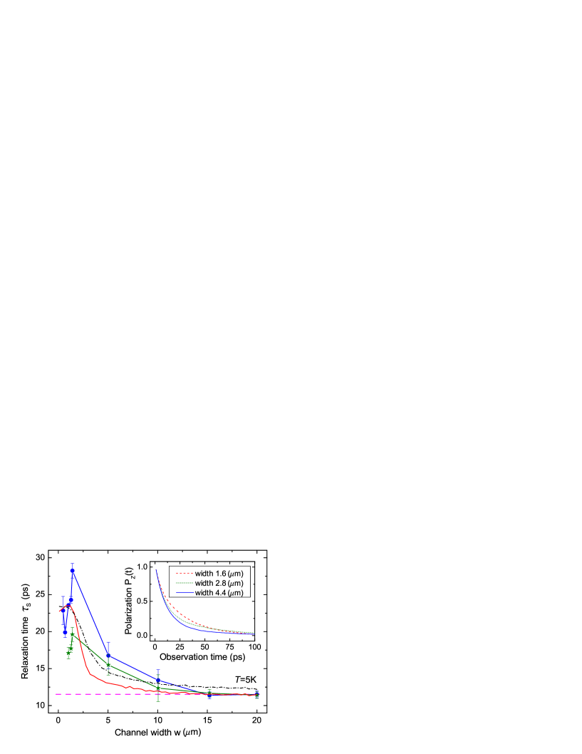
Figure 1: (Color online) The spin relaxation times $\tau_{s}$’s of $[1,0,0]$ sample (circle) and $[1,1,0]$ sample (star) versus channel width $w$ are taken from the experiments in Ref. Awschalom . The $\tau_{s}$ calculated by the SPI method are extracted from the polarization curve $P_{z}(t)$, fitted by Eq. (6) with free parameters $A$ and $c$ (red solid curve) and with fixed parameters $A=1$ and $c=0$ (black dash-dotted curve). The experimental $\tau_{s}$ saturates at $11.5\,\mu$m (pink dashed straight line) for large $w$, the same as the analytically estimated value for $L_{so}=2.19\,\mu$m. The inset demonstrates three examples of $P_{z}(t)$ for channel width $w=1.6\,\mu$m, $2.8\,\mu$m, and $4.4\,\mu$m.

Since the width range $0.4\,\mu$m $\leq w\leq 20\,\mu$m used in our calculations is much larger than the de Broglie wavelength $\lambda_{f}$, the quantum effects are negligible and the validity of the SPI approach is justified. With the above experimental parameters, the SPI calculations are represented in Fig. 1, where the inset shows the relaxation curves $P_{z}(t)$ for three channels of different widths. All electron spins were initially aligned in $z$-direction. The relaxation time $\tau_{s}$ can be determined by a fitting of these $P_{z}(t)$ curves with the exponential function

$$P_{z}(t)=A\exp(-t/\tau_{s})+c.$$ (6)

For example, the (red) solid curve in Fig. 1 represents the relaxation time of $1.2\times 10^{7}$ electrons in channels of different widths $w$’s. A comparison with the experimental data (circles and stars) leads to following conclusions:

• At large widths ($w>15$ $\mu$m), the electron spin can be regarded as relaxing in bulk systems. In the experiments in Ref. Awschalom, , $l_{SP}$ was estimated to be $1.0\pm 0.1\,\mu$m, corresponding to $L_{so}=2.0\pm 0.2\,\mu$m. This experimental uncertainty results in $\tau_{s}=9.7\pm 2.1$ ps, when calculated by the SPI method. However, each $\tau_{s}$ obtained from the SPI method agrees very well with that determined by the analytical expression of DP relaxation $\tau_{s}=L_{so}^{2}/(4v_{F}\,l)$ for boundless systems. Thus, if the experimental samples are governed by pure Rashba Hamiltonian, as in our calculation, these samples most likely have $L_{so}=2.19\,\mu$m. This value is used in our SPI simulations to obtain the red and black curves in Fig. 1.

• For intermediate widths ($1.4\,\mu$m$<w<15\,\mu$m), there is no an analytical expression for $\tau_{s}$ to compare with. The SPI result deviates slightly from the experimentally measured $\tau_{s}$. The maximum deviation is around 3 ps for $[1,1,0]$ sample and 4 ps for $[1,0,0]$ sample at $w=5\,\mu$m. The calculated $\tau_{s}$ is closer to the $\tau_{s}$ of the $[1,1,0]$ sample.

• For small widths ($w<1.4\,\mu$m), the experimentally measured $\tau_{s}$ saturates at $28$ ps for $[0,0,1]$ sample and $20$ ps for $[0,1,1]$ sample. It is assumed in Ref. Awschalom, that this saturation might be related to other mechanisms, like the bulk inversion asymmetry. However, the calculated $\tau_{s}$ in Fig. 1 is also bounded by a maximum value around $24$ ps, although in our calculation only the Rashba Hamiltonian was considered, without any additional mechanisms involved.

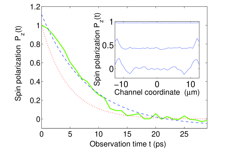
Figure 2: (Color online) In the inset, a spin configuration in a channel of the length $8\pi\;\mu$m relaxes to zero, depicted at three different times. These configurations are spatially uniform up to the ripples at two ends caused by boundary effect. Recording the polarization $P_{z}(t)$ at the middle point of the channel gives the relaxation curve (green solid thick) in the main plot. This curve can be fitted by the exponential function in Eq. (6) with $[\tau_{s},A,c]=[7.127,\,1.274,\,-0.055]$ (blue dashed curve) and $[\tau_{s},A,c]=[4.323,\,1,\,0]$ (red dotted curve). For $t$ close to zero, most electrons have not been reflected by impurities or boundaries. In this range $P_{z}(t)$ does not behave as an exponential function. Later, after most of the electrons and their spins have been randomized by impurities or boundaries, $P_{z}(t)$ became more exponential-like. The physical parameters used are $[w,L_{so},v_{F},l]=[0.1\,\mu{\rm m},2\,\mu{\rm m},0.37\,\mu{\rm m/ps},0.3\,\mu{\rm m}]$ with $6\times 10^{4}$ electrons.

An important factor affecting the interpretation of the experimental data is how to determine the relaxation time $\tau_{s}$ from the function $P_{z}(t)$. The solid curve in Fig. 2 is an example of $P_{z}(t)$ in a channel with $w=0.1\,\mu$m and $l=0.3\,\mu$m. At first sight it looks like an exponential function to be fitted with a relaxation time $\tau_{s}$ in Eq. (6). But a closer look shows that it is not a pure exponential function. Indeed, if we gradually increase $l$ by reducing the number of impurities in the channel, the monotonically decreasing $P_{z}(t)$ in Fig. 2 will transform to an oscillatory function. In the extreme case of an infinitely thin impurity-free channel, we shall prove in the next section that the evolution of $P_{z}(t)$ will follow the Bessel function

$$P_{z}(t)=J_{0}\left(\frac{2v_{F}\,t}{L_{so}}\right).$$ (7)

This analytical formula is depicted by the smooth (red) dashed curve in Fig. 3. A corresponding result of a numerical SPI simulation is plotted as a (green) rugged solid curve in the same figure.

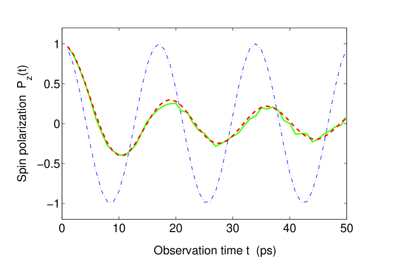
Figure 3: (Color online) In a 1D channel without impurities, a spin polarization $P_{z}(t)$ behaves like a sinusoidal function Eq. (8) (blue dash-dotted curve). In an infinitely thin channel without impurities, $P_{z}(t)$ behaves like a Bessel function Eq. (7) (smooth red dashed curve), which agrees with the numerically obtained $P_{z}(t)$ simulated by $5\times 10^{4}$ electrons (rugged green solid curve). The physical parameters are $[w,L_{so},v_{F},l]=[0.1\,\mu{\rm m},2\,\mu{\rm m},0.37\,\mu{\rm m/ps},10^{4}\,\mu{\rm m}]$.

During transition from the diffusive to the ballistic regime, $P_{z}(t)$ will undergo a crossover from an exponential to a Bessel function. In principle, it is meaningless to use an exponential function to extract $\tau_{s}$ from such a crossover function, especially when it is far from an exponential behavior. But if one would like to carry out this procedure, the so obtained $\tau_{s}$ will depend on the choice of the parameters $A$ and $c$ in Eq. (6):

• If $A=1$ is chosen, Eq. (6) can precisely fit the real initial polarization $P_{z}(t)=1$ at $t=0$ (red dotted curve in Fig. 2).

  If $A\neq 1$, Eq. (6) can provide a better fitting to $P_{z}(t)$ in a wider range of times at $t>0$ (blue dashed curve in Fig. 2). On this reason, such a choice of A seems to be more appropriate.

• Further, if $c\neq 0$ the fitted values of $c$ and $\tau_{s}$ will be strongly dependent on the observation time cutoff. The reason is that usually the tail of $P_{z}(t)$ is oscillating, if the system within the considered range of times is not in the diffusive regime. The closer the system to the ballistic regime, the larger is the oscillation amplitude. The Bessel function in Eq. (7) for ‘pure’ ballistic regime has the largest amplitude. If the non-oscillating Eq. (6) is used to fit an oscillating Eq. (7) truncated at some cutoff, the fitted $\tau_{s}$ and $c$ will depend on the cutoff. The corresponding uncertainty of $\tau_{s}$ will decrease with an increasing observation time.

In the experiments Awschalom , the width of the channel varies between $w\approx 1.5\,l$ and $70\,l$. Since at the smallest $w$ the system is not far from the ballistic regime, the difference between $P_{z}(t)$ and the exponential function should be observable. Indeed, the value of $\tau_{s}$ fitted by Eq. (6) with $A=1$ and $c=0$ (black dash-dotted curve in Fig. 1) is somewhat distinct from $\tau_{s}$ at $A\neq 1$ and $c\neq 0$ (red solid curve in Fig. 1). Since our observation time is sufficiently long, the fitted value of $c$ is close to zero. A disagreement produced by different fitting procedures will become more remarkable when the system approaches the ballistic regime with strongly oscillating $P_{z}(t)$. Hence, when comparing $\tau_{s}$’s obtained by different research groups, it is important to know the whole set of the fitting parameters ($A$, $c$, and observation time). Even when the same $P_{z}(t)$ curve is considered, the reported $\tau_{s}$’s could be different. One more problem with the fitting procedure is that even in the diffusive regime the evolution of the spin polarization not necessarily follows the exponential behavior with a single relaxation time. For example, a homogeneous $P_{z}$ distribution is not an eigenstate of the diffusion equation in a 2D channel. Therefore, as shown in Ref. Schwab, , edge states can contribute to the $P_{z}(t)$ evolution with the relaxation time different from that of the bulk eigenstate. The weight of edge states increases with decreasing $w$.

In regime (ii), the experimental data deviate slightly from the SPI calculations with a maximum difference $\tau_{s}\approx 3\sim 4$ ps at $w\approx 5\,\mu$m. This discrepancy is too large to be attributed to different fitting procedures. One of the explanations for such a behavior might be a specific role of long-lived edge states. The lifetime of such modes depends on the boundary conditions Schwab . Our SPI calculations assumed a specular reflection of electrons from hard wall boundaries of the wire. Probably, the experimental situation in Ref.Awschalom, corresponds to other boundary conditions which give rise to the edge states with larger $\tau_{s}$. This problem requires a more thorough analysis.

In regime (iii), the relaxation time goes to a finite value at $w\rightarrow 0$ in both experimental and SPI calculated plots in Fig. 1. For a homogeneous spin distribution along the channel, the diffusion theory Malshukov also predicts a saturation of $\tau_{s}$ at $w\rightarrow 0$. The saturated value should be twice of the bulk DP spin relaxation time. With the experimental bulk value $\tau_{s}$=11.5 ps, one expects $\tau_{s}$=22.8 ps at $w=0$. Experimental and SPI curves at Fig.1 are not far from this value, although the diffusion approximation fails at $w\simeq l$. At the same time, one should not forget that in a narrow channel the time evolution of the spin polarization strongly deviates from the exponential function. On this reason, in regime (iii) $\tau_{s}$ can not be a representative parameter to describe the spin relaxation.

IV IV Bessel relaxations in ballistic channels

Depending on the ratio between the channel width and the electron wavelength, one encounters two limiting cases. If the wire carries only one propagating channel, we have effectively a 1D situation. In the opposite limit, if the width of the wire is much larger than the electron wavelength, semiclassical electrons are able to move in both $x$- and $y$-directions. Therefore, the system is two-dimensional, even if geometrically the channel is narrow, with $w$ much less than other characteristic lengths, such as $L_{so}$ and $l$. Below, we will consider the evolution of electron polarization in the ballistic regime for these two limiting cases.

IV.1 1D ballistic channels

Let us consider a 1D impurity-free channel where at $t=0$ spins of all electrons are aligned in $z$-direction. Since impurities and the electron-electron interaction are absent, electrons can only move in $+x$ or $-x$ directions along the channel axis with a constant velocity. The spins of all these electrons will rotate simultaneously along different geodesics connecting the north and south poles on the spin sphere. A $2\pi$ spin rotation takes place when an electron passes a distance $\pi L_{so}$ during a time period $\pi L_{so}/v_{F}$. Therefore, the angular frequency of this rotation is $2\,v_{F}/L_{so}$, the same for all spins. The spin polarization at any place in the channel will then evolve according to

$$P_{z}(t)=\cos\left(\frac{2\,v_{F}\,t}{L_{so}}\right)$$ (8)

and oscillate without any amplitude decay, as shown by the blue dash-dotted curve in Fig. 3.

IV.2 2D ballistic channels

Now we suppose that the channel is a 2D thin ballistic wire where all electron spins are initially aligned in the $z$-direction, as in the 1D case. Given an observation point, say $p_{0}(x_{0},\,y_{0})$ in Fig. 4, the polarization $P_{z}(t)$ at $x_{0}$ at time $t$ is the average of the spins of all electrons which will arrive at this moment at the $x_{0}$ cross section. These electrons can arrive through a straight trajectory $\overline{p_{1}p_{0}}$ of length $l=v_{F}t$, or through different zigzag trajectories of the same length, as the path $\widetilde{p_{2}p_{0}}$ in Fig. 4.

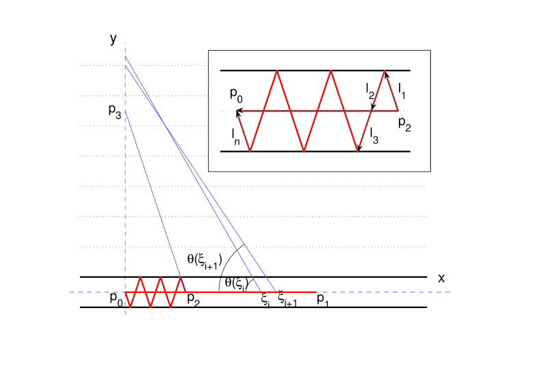
Figure 4: (Color online) Two kinds of trajectories with the same length $l=v_{F}t$ in a thin channel: the straight trajectory $\overline{p_{1}p_{0}}$ and the zigzag trajectory $\widetilde{p_{2}p_{0}}$. The latter has the same length as the straight line $\overline{p_{2}p_{3}}$, since it can be obtained through a multiple mirror reflection of $\overline{p_{2}p_{3}}$ with respect to the horizontal dotted lines. The symbol $\theta(\xi)$ denotes a certain outgoing angle of an electron located at $\xi$, as explained in the text. The trajectory $\widetilde{p_{2}p_{0}}$ is magnified in the inset.

As follows from Eq. (3), the spin state of an electron running along the zigzag trajectory $\widetilde{p_{2}p_{0}}$ in the inset of Fig. 4 will evolve according to the spin evolution operator

$$U_{\widetilde{p_{2}p_{0}}}=\exp\left(\!-i\,\frac{\bm{l}_{n}\!\cdot\!\bm{\sigma}}{L_{so}}\right)...\exp\left(\!-i\,\frac{\bm{l}_{2}\!\cdot\!\bm{\sigma}}{L_{so}}\right)\exp\left(\!-i\,\frac{\bm{l}_{1}\!\cdot\!\bm{\sigma}}{L_{so}}\right)$$

$$=\left[\bm{1}-i\,\frac{\bm{l}_{n}\!\cdot\!\bm{\sigma}}{L_{so}}+\!...\right]\!...\!\left[\bm{1}-i\frac{\bm{l}_{2}\!\cdot\!\bm{\sigma}}{L_{so}}+\!...\right]\!\left[\bm{1}-i\,\frac{\bm{l}_{1}\!\cdot\!\bm{\sigma}}{L_{so}}+\!...\right]$$

$$=U_{\overline{p_{2}p_{0}}}+O\left(\frac{w^{2}}{L_{so}^{2}}\right),$$ (9)

Making the above expansion up to the linear in $w$ term, the operator $U_{\overline{p_{2}p_{0}}}$ can be written as

$$U_{\overline{p_{2}p_{0}}}:=\exp\left(-i\,\frac{\bm{l}\cdot\bm{\sigma}}{L_{so}}\right)=\left[\bm{1}-i\,\frac{\sum_{j=1}^{n}\bm{l}_{j}\cdot\bm{\sigma}}{L_{so}}+...\right],$$

with the vector ${\bm{l}}$ pointing from $p_{2}$ to $p_{0}$. Equation (IV.2) indicates that the spin evolution of an electron moving along the zigzag trajectory $\widetilde{p_{2}p_{0}}$ is approximately the same as that of an electron drifting along the shorter straight line $\overline{p_{2}p_{0}}$ with a drift velocity $v_{F}x/l$ slower than $v_{F}$, where $l=|\bm{l}_{1}|+|\bm{l}_{2}|+...+|\bm{l}_{n}|$ and $x=|\bm{l}_{1}+\bm{l}_{2}+...+\bm{l}_{n}|$. As discussed in the previous subsection, if an electron moves a distance $x$, its spin will rotate the angle $2x/L_{so}$ in the spin space. If initially this spin is aligned along the z-direction, its z-component will become

$$s_{z}(x)=\cos\left(\frac{2x}{L_{so}}\right)+O\left(\frac{w^{2}}{L_{so}^{2}}\right).$$ (10)

To determine how many electrons will contribute to $P_{z}(t)$, let us uniformly divide the channel axis into small intervals $[\xi_{i},\,\xi_{i+1}]$ of length $\varepsilon$ separated by points $\xi_{i}$ with $i=0,\,1,\,2,\,...$. Let $\theta(\xi_{i})$ be the outgoing angle of an electron at $\xi_{i}$. This angle is chosen so that when the electron travel a zigzag path of the length $l=v_{F}t$, its drift length will be $x$. Hence, this electron will arrive at $p_{0}$ at time $t$. If outgoing angles are isotropically distributed, the number of such electrons within $[\xi_{i},\,\xi_{i+1}]$ is proportional to the spanned angle $W(\xi_{i})=\theta(\xi_{i})-\theta(\xi_{i+1})$. For a given small interval $\varepsilon=\xi_{i+1}-\xi_{i}$ this angle is related to $x$ by

$$W(x)\! = \!\theta(x)-\theta(x+\varepsilon)=\arccos\left(\frac{x}{l}\right)\!-\arccos\left(\frac{x+\varepsilon}{l}\right)$$ (11)

$$= \frac{\varepsilon}{\sqrt{l^{2}-x^{2}}}+O\left(\frac{\varepsilon}{l}\right),$$

where the outgoing angle $\theta(x)$ of the trajectory along $\widetilde{p_{2}p_{0}}$ is the same as the angle of $\overline{p_{2}p_{3}}$ (see Fig. 4). According to Eq. (5), the spin polarization $P_{z}(t)$ at $p_{0}$ will be contributed from electrons traveling from different initial locations $x$:

$$P_{z}(t)=\frac{\displaystyle\int_{0}^{l}\rho\,W(x)\,s_{z}(x)\,dx}{\displaystyle\int_{0}^{l}\rho\,W(x)\,dx},$$ (12)

where $\rho$ is the line density of electrons along the channel axis. Inserting Eq. (10) and (11) into Eq. (12) yields

$$P_{z}(t) = \frac{\displaystyle\int_{0}^{l}\frac{\varepsilon}{\sqrt{l^{2}-x^{2}}}\,\cos\left(\frac{2x}{L_{so}}\right)dx}{\displaystyle\int_{0}^{l}\frac{\varepsilon}{\sqrt{l^{2}-x^{2}}}\;dx}$$

$$= J_{0}\left(\frac{2v_{F}\,t}{L_{so}}\right)+O\left(\frac{w^{2}}{L_{so}^{2}}\right),$$

which at the $w\rightarrow 0$ limit is the Bessel function in Eq. (7). Hence, uniformly polarized spins in a ballistic narrow channel will relax to the zero polarization through a Bessel function. This phenomenon is in contrast to our conventional intuition that a relaxation is a monotonically exponential process. It is worthwhile to note that the Bessel-like spin dynamics also takes place in other SOI systems.Culcer

We conclude that the spin relaxation dynamics even in a very thin 2D channel is remarkably different from that in a 1D channel, as can be seen from a comparison of Eq. (7) with Eq. (8). It can be understood from the fact that no matter how narrow the width of a 2D channel is, it contains a large number of electrons moving along various zigzag trajectories bouncing between two channel boundaries. These trajectories give a significant contribution and change the dynamics of $P_{z}(t)$ from a sinusoidal oscillation in 1D systems to a Bessel-function decay in 2D systems.

V V Relaxation of helix spin modes

In previous sections, all initial electron spins were polarized along the $z$-axis. The relaxation dynamics of such spin configuration does not change dramatically at small $w$ (the maximum $\tau_{s}$ only reaches 28 ps in Fig. 1.), in agreement with the experiment.Awschalom . In fact, this behavior is expected from the analysis of eigenstates of the spin diffusion equation. As shown in Ref. Malshukov, , the only homogeneous eigenstate is $\Psi_{0}$ in Fig. 5(a), which has all spins polarized in the $y$-direction and whose relaxation time strongly increases in narrow wires. In addition to this mode there are two nonuniform slowly relaxing eigenstates.

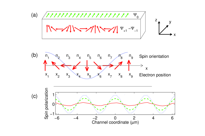
Figure 5: (Color online) (a) Long-lived spin eigenmodes: $\Psi_{0}$ denotes the spin mode with all spins aligned in $y$-direction. $\Psi_{+1}-\Psi_{-1}$ represents the helix spin modes with spin rotating on the xz-plane. (b) An electron in the channel moves a distance $\pi L_{so}$ from the left end $x_{1}$ to the right end $x_{9}$. Due to Rashba SOI, the spin of the electron precesses from $\bm{n}_{1}$ to $\bm{n}_{9}$ and completes a phase period of $2\pi$. (c) A schematic plot of the decay of the helix mode at $1$ (dotted), $35$ (dash), and $170$ (solid) time units. $\Psi_{\pm 1}$ in Fig. 5(a) has been replaced by $\Psi_{+1}-\Psi_{-1}$.

These two long-lived eigenmodes exist in a 2D channel where $w\ll l_{SP}$. Using a perturbation method with respect to $w/l_{SP}$, one can solve a diffusion equation and obtain its unperturbed eigensolution Malshukov

$$\widetilde{\psi}_{M,k,m}(x,y)=\exp(ikx)\chi_{m}(y)\Psi_{M},$$ (13)

with the eigenvalue (relaxation rate)

$$\Gamma^{0}_{M,k,m}=D(\pi m/d)^{2}+D(k-Ml_{SP}^{-1})^{2}.$$ (14)

Therein, $\Psi_{M}$ are the eigensolutions of the momentum operator $J_{y}$ with eigenvalues $M=0,\pm 1$ and $\chi_{2n}(y)=\cos(2\pi yn/d)$, as well as $\chi_{2n+1}(y)=-\sin[\pi y(2n+1)/d]$. In Fig. 5(a), $\Psi_{\pm 1}$ will construct the helix eigenmodes with the wave vectors $k=\mp 1/l_{SP}$. We note that the eigenmode of the diffusion equation is a spin configuration exponentially decreasing in time, but its shape remaining unchanged. Taking the second order correction in $w/l_{SP}$, one obtains

$$\Gamma_{M,k,m} = \Gamma^{0}_{M,k,m}+\frac{(2-M^{2})w^{2}}{24\tau_{s0}\;l_{SP}^{2}}$$ (15a)

$$= \Gamma^{0}_{M,k,m}+\frac{2(2-M^{2})w^{2}v_{F}l}{3L_{so}^{4}}$$ (15b)

for $\mid k-M/l_{SP}\mid\ll 1/l_{SP}$, where $\tau_{s0}=l_{SP}^{2}/v_{F}l$ and $l_{SP}=L_{so}/2$ have been used in the second equality. The modes with $m=0$, and $k=M/l_{SP}$ will relax most slowly, since in these cases the first term $\Gamma^{0}_{M,k,m}$ in Eq. (15) disappears. The second term indicates that the spin relaxation time $\tau_{s}=1/\Gamma_{M,k,m}$ will be proportional to $1/w^{2}$. In the limit $L_{so}\gg w$, we thus have $\tau_{s}$ much larger than the D’yakonov Perel’ relaxation time $\tau_{s0}$ in 2D boundless systems.DP Such a behavior will become more clear from the following simple consideration in a 1D system. Let us consider an electron at $x_{1}$ in a 1D channel with an initial spin pointing to $\bm{n}_{1}$, as shown in Fig. 5(b). Under the Rashba SOI, the spin will rotate to $\bm{n}_{2}$, $\bm{n}_{3}$, …, when this electron moves to $x_{2}$, $x_{3}$, …. It is easy to see that if each electron spin in an initial spin density distribution follows this ($x_{i},\,\bm{n}_{i}$) relation, such a distribution will not change in time. Hence, its relaxation time is infinite. In a realistic 2D wire the relaxation time is finite at finite width. That is because electrons there can move in the y-direction. The polarization $P_{z}(t)$ contributed from electrons moving along the channel is frozen, as in the 1D case, while electrons moving along the the y-axis give rise to the relaxation of the helix distribution.

Since the above expressions have been obtained under the assumption $l\ll w\ll L_{so}$, it is interesting to extend the analysis beyond this limits. Within the SPI method we studied the relaxation of the helix mode in the range $l\lesssim w$, choosing $L_{so}=12.5\,\mu$m, $l=0.5\,\mu$m, and $v_{F}=0.37\mu$m/ps. Given the initial helix spin mode $\Psi_{+1}-\Psi_{-1}$ corresponding to spins oriented along the z-axis at $x$=0 in Fig. 5(a), the spin relaxation time $\tau_{s}(w)$ calculated by the SPI method is represented by squares in the inset of Fig. 6. In the range of $w<10\,\mu$m, this time increases dramatically and strongly deviates from the $\tau_{s}$ of the corresponding uniform mode (red solid curve). Note that in order to display the divergent $\tau_{s}$, we choose a large $\tau_{s}$-axis scale in the inset of Fig. 6. At this scale the uniform mode $\tau_{s}$ (red curve) almost overlaps with the $\tau_{s}=0$ axis. The relaxation time of the uniform mode will saturate at some value for $w\rightarrow 0$. It is $\tau_{s}\approx 28$ ps for $[L_{so},\,l,\,w]=[2.19,\,0.28,\,1.4]\,\mu$m in Fig. 1 and $\tau_{s}\approx 441.1$ ps for $[L_{so},\,l,\,w]=[12.5,\,0.5,\,0.4]\,\mu$m. In contrast to these uniform modes, $\tau_{s}$ of the helix mode strongly increases for $w\rightarrow 0$ (if $w\gg l$). This behavior is consistent with the theoretical result Eq. (15a). On the other hand, if $w$ is as large as $20\,\mu$m, the relaxation time $\approx 1927.4$ ps of the helix mode is still much larger than $\tau_{s}\approx 241.0$ ps corresponding to the uniform mode. This difference can be easily seen by magnifying the $\tau_{s}$-axis of the inset in Fig. 6.

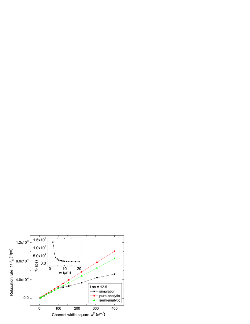
Figure 6: (Color online) The relaxation time $\tau_{s}$ of the uniform mode (red solid) and the helix mode (black square) versus the channel width $w$ in the inset. For small $w$, the square curve of the helix mode is redrawn as $1/\tau_{s}$ against $w^{2}$ in the main plot, to compare with the $\tau_{s}$’s derived from the analytical formula (15b) (red circle) and the semi-analytical formula (15a) (green triangular).

The main plot in Fig. 6 shows the $1/\tau_{s}$ dependence on $w^{2}$. The squares show the helix relaxation rate corresponding to the data in the inset. The line with circles for the helix mode is obtained from the analytical expression Eq. (15b), while the line with triangles is obtained from Eq. (15a). In the latter line, $\tau_{s0}$ is simulated numerically, instead of using the analytical relation $\tau_{s0}=l_{SP}^{2}/v_{F}l$ mentioned below Eq. (15b). The lines with circles and triangles are valid only at $l\ll w\ll L_{so}$, while that with squares is valid for all $w$. One can clearly see that the curve calculated by the SPI method agrees very well with Eq. (15) at small $w$ between $w_{1}=2\,\mu$m (the smallest calculated width) and $w_{2}=10\,\mu$m. It is interesting to note that although formula Eq. (15) was derived under the condition $l\ll w\ll L_{so}$, it seems to be valid in a wider range of $w$, because $w_{1}$ is close to the ballistic regime crossover point at $w\sim l=0.5\,\mu$m and $w_{2}$ is close to $L_{so}=12.5\,\mu$m. Finally, one should not expect that the linear trend in Fig. 6 can continue down to $w^{2}\rightarrow 0$ because in this range the system will eventually reach the ballistic regime and $P_{z}(t)$ will decay like a crossover function between the exponential and the Bessel functions. Similar to the discussion of the uniform initial spin configuration in Section III, it does not make sense to consider $\tau_{s}$ at extremely small $w$, because $P_{z}(t)$ is no longer an exponential function.

VI VI Conclusion

The semiclassical path integral method has been applied to study the spin relaxation in thin 2D wires with the Rashba spin-orbit interaction. We considered the relaxation of a uniform spin polarization along the $z$-axis, as well as of the long-lived helix mode. In the former case we found a good agreement of $\tau_{s}$ calculated in the regime of large $w$ ($w\approx 20\,\mu$m) with the well known bulk DP spin relaxation rate and with the experimental data from Ref. Awschalom, . At smaller $w$ our numerical results deviate slightly from the experimental data. The nature of this distinction is not clear. We assume that the edge spin diffusion modes can contribute to the spin relaxation, so that the conditions for electron reflections from the wire lateral boundaries become important. Also, the Dresselhaus spin-orbit interaction can give rise to the observed dependence of $\tau_{s}$ on the orientation of the wire axis in the xy-plane. At $w\rightarrow 0$ the relaxation time has a tendency to saturate at a value which is about twice of the bulk $\tau_{s}$, as predicted by the spin diffusion theory. Although both SPI and experimental data show similar saturation behavior, one must take into account that at $w$ approaching the crossover $w\sim l_{f}$ to the ballistic regime the evolution of the spin polarization can not be described by an exponential function. Hence, in this regime $\tau_{s}$ is not a representative parameter to describe the spin relaxation. We studied the evolution of the spin polarization in the ballistic regime and found that it is described by the Bessel function. The numerical SPI results fit well to this behavior. For the helix spin distribution, the linear dependence of $1/\tau_{s}$ on $w^{2}$ predicted in the framework of the diffusion theory Malshukov coincides precisely with that calculated by the SPI method. The SPI method also allowed to calculate the spin relaxation beyond the constraints of those analytic results. Malshukov

This work is supported by the National Science Council in Taiwan through Grant No. NSC 96-2112-M-009-003 and Russian RFBR Grant, No 060216699.

References

- (1) S. A. Wolf et al., Science 294, 1488 (2001); I. Zütic, J. Fabian, S. D. Sarma, Rev. Mod. Phys. 76, 323 (2004); G. A. Prinz, Phys. Today 48(4), 58 (1995)
- (2) M. I. D’yakonov and V. I. Perel’, Sov. Phys. Solid State 13, 3023 (1971).
- (3) C.-H. Chang, A. G. Mal’shukov, and K. A. Chao, Phys. Rev. B 70, 245309 (2004).
- (4) A. G. Mal’shukov and K. A. Chao, Phys. Rev. B 61, R2413 (2000).
- (5) A. A. Kiselev and K. W. Kim, Phys. Rev. B 61, 13 115 (2000).
- (6) P. Schwab, M. Dzierzawa, C. Gorini, and R. Raimondi, Phys. Rev. B 74, 155316 (2006)
- (7) A. W. Holleitner, V. Sih, R. C. Myers, A. C. Gossard, and D. D. Awschalom, Phys. Rev. Lett. 97, 036805 (2006).
- (8) C.-H. Chang, A. G. Mal’shukov, and K. A. Chao, Phys. Lett. A 326, 436 (2004).
- (9) A.G. Mal’shukov, V.V. Shlyapin and K. A. Chao, Phys. Rev. B 66, 081311(R) (2002).
- (10) H. Chen, J. J. Heremans, J. A. Peters, A. O. Govorov, N. Goel, S. J. Chung, and M. B. Santos, Appl. Phys. Lett. 86, 032113 (2005).
- (11) D. Culcer and R. Winkler, Phys. Rev. B 76, 195204 (2007).