Non-local Andreev reflection under ac bias

Abstract

We theoretically analyze non-local electron transport in multi-terminal normal-metal-superconductor-normal-metal (NSN) devices in the presence of an external ac voltage bias. Our analysis reveals a number of interesting effects, such as, e.g., photon-assisted violation of balance between crossed Andreev reflection (CAR) and elastic cotunneling (EC). We demonstrate that at sufficiently small (typically subgap) frequencies of an external ac signal and at low temperatures the non-local conductance of the NSN device turns negative implying that in this regime CAR contribution to the non-local current dominates over that of EC. Our predictions can be directly tested in future experiments.

1 Introduction

The phenomenon of non-local (or crossed) Andreev reflection [1, 2] is known to occur in multi-terminal hybrid normal-metal-superconductor-normal-metal (NSN) proximity structures and involves two subgap electrons entering a superconductor from two different normal terminals and forming a Cooper pair there. Such crossed Andreev reflection (CAR) manifests itself, e.g., in the dependence of the current $I_{1}$ through the left NS interface of an NSN structure on the voltage $V_{2}$ across the right NS interface. As a result, the non-local conductance $G_{12}=-\partial I_{1}/\partial V_{2}$ of an NSN device differs from zero and can be detected experimentally. Various aspects of this intriguing phenomenon have recently become a subject of intensive investigations both in experiment [3, 4, 5, 6] and in theory, see, e.g., [7, 8, 9, 10, 11, 12, 13, 14, 15, 16, 17, 18, 19] and further references therein.

It is important that CAR is not the only process which contributes to the non-local conductance $G_{12}$. Another relevant process is direct electron transfer between two normal terminals through the superconductor. In the tunneling limit this process is just the well known elastic cotunneling (EC). It was demonstrated [7] that in the lowest order in tunneling the contributions from EC and CAR to $G_{12}$ exactly cancel each other in the limit of low temperatures and voltages, i.e. the non-local conductance $G_{12}$ tends to zero in this limit. In certain cases this observation might complicate experimental identification of CAR in NSN structures with weakly transmitting interfaces.

Despite such possible complications in experiments [3, 4, 5, 6] the non-local signal $G_{12}$ was successfully detected both at high and low temperatures showing a rich structure of non-trivial features. Some of these features are currently not yet fully understood and are still waiting for their adequate theoretical interpretation. These observations – along with various theoretical predictions – also demonstrate that the exact cancellation between EC and CAR contributions [7] can be violated in a number of ways. One of them is simply to lift the spin degeneracy in the problem, e.g., by considering NSN structures with spin-active interfaces [14] or by using ferromagnets (F) instead of normal electrodes [9]. Experiments with FSF structures [3] directly demonstrated the dependence of the non-local conductance $G_{12}$ on the polarization of F-electrodes.

In a spin degenerate case the non-local conductance $G_{12}$ does not vanish beyond the tunneling limit [12, 14], i.e. the cancellation between EC and CAR terms is effectively eliminated due to higher order electron tunneling processes which become significant at higher barrier transmissions. This theory predicts positive non-local conductance implying that direct electron transfer should always dominate over CAR at higher barrier transmissions. Furthermore, for ballistic NSN structures CAR was predicted to vanish completely in the limit of fully open NS interfaces [12, 14].

It is worth pointing out that both positive and negative non-local signals have been detected in multi-terminal NSN devices [3, 4, 6]. It was argued [15] that negative non-local currents could possibly be attributed to the effect of electron-electron interactions. In the presence of strong Coulomb interaction negative non-local conductance was obtained in single-level quantum dots coupled to normal and superconducting electrodes [18]. In general, this important issue deserves a detailed theoretical investigation which should account for non-trivial interplay between disorder and Coulomb interaction. Previously a similar analysis was developed for (local) Andreev reflection in NS hybrid structures [20, 21, 22]. This analysis revealed a number of interesting features which can also significantly affect non-local properties of NSN devices.

Leaving this important issue for future investigations, here we address a somewhat different situation. Namely, we will study both EC and CAR processes in NSN structures in the presence of an external ac bias. We will demonstrate that application of an ac electromagnetic field to such structures lifts exact cancellation between EC and CAR contributions already in the lowest order in barrier transmissions. Under certain conditions CAR can dominate over EC, in which case the non-local conductance of the system $G_{12}$ turns negative.

2 Non-local currents in NSN devices

We will analyze the behavior of multi-terminal NSN structures. An example of such a structure is schematically shown in Fig. 1: A long superconducting wire with BCS order parameter $\Delta(T)$ (connected to bulk superconducting terminals) is coupled to two normal metals via tunnel barriers with resistances $R_{1}$ and $R_{2}$. We also assume that time dependent voltages $V_{1}$ and $V_{2}$ are applied to normal metal terminals.

The Hamiltonian of this system can be expressed in the form

$$H=H_{1}+H_{2}+H_{S}+H_{1,T}+H_{2,T},$$ (1)

where

$$H_{r}=\sum_{\alpha=\uparrow,\downarrow}\sum_{k}\big{(}\epsilon_{k}-eV_{r}(t)\big{)}c^{\dagger}_{r,k,\alpha}c_{r,k,\alpha},$$ (2)

are the Hamiltonians of the normal leads ($r=1,2$),

$$H_{S}=\sum_{k}\big{[}\xi_{k}(a_{k,\uparrow}^{\dagger}a_{k,\uparrow}+a_{k,\downarrow}^{\dagger}a_{k,\downarrow})+\Delta(a^{\dagger}_{k,\uparrow}a^{\dagger}_{k,\downarrow}+a_{k,\downarrow}a_{k,\uparrow})\big{]}$$ (3)

is the Hamiltonian of the superconducting electrode and

$$H_{r,T}=\sum_{\alpha=\uparrow,\downarrow}\sum_{k,p}\big{[}t_{kp}c_{r,k,\alpha}^{\dagger}a_{\alpha,p}+\,{\rm c.c.}\,\big{]}$$ (4)

are the tunnel Hamiltonians describing electron transfer between normal terminals and a superconductor. In what follows we will restrict our analysis to the spin-degenerate case and will also ignore inelastic effects.

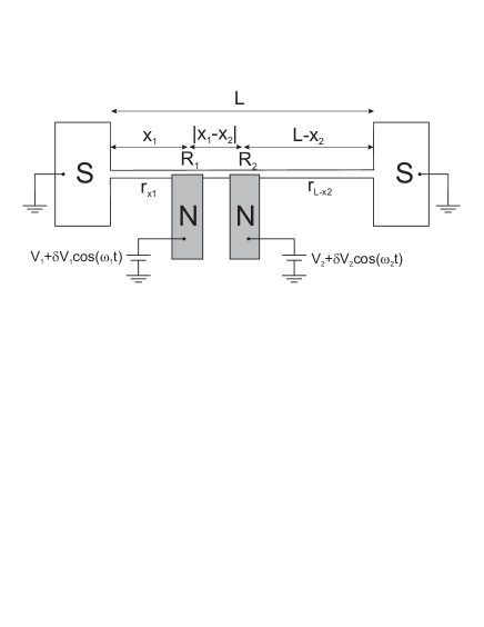
Figure 1: Schematics of the system under consideration. A long superconducting wire is coupled to two normal metal leads via the two tunnel junctions with the resistances $R_{1}$ and $R_{2}$.

In order to evaluate the non-local current response to the applied voltages we proceed within the standard perturbative approach in the tunnel Hamiltonians $H_{1,T}$ and $H_{2,T}$ combined with the Keldysh technique. The whole calculation is analogous to that performed in Ref. [7] with the only important difference that here the applied voltages $V_{1,2}$ explicitly depend on time. Calculating the current $I_{1}$ across the first barrier perturbatively in the corresponding tunneling amplitudes, we obtain

$$I_{1}(V_{1},V_{2})=I_{1}^{(0)}(V_{1})+I_{11}(V_{1})+I_{12}(V_{2}),$$ (5)

where the first two terms $I_{1}^{(0)}(V_{1})$ and $I_{11}(V_{1})$ represent the standard contributions to the current across NS interface evaluated respectively in the first and second orders in the interface transmission, while the term $I_{12}(V_{2})$ describes the non-local contribution to the current across the first junction due to the presence of the voltage bias $V_{2}$ at the second normal terminal. For these three contributions we find

$$I_{1}^{(0)} = \frac{e}{2}\,{\rm tr}\,\big{[}-\check{G}_{1}\check{t}_{1}\check{G}_{S}\check{t}^{\dagger}_{1}\check{\Lambda}+\check{G}_{S}\check{t}_{1}^{\dagger}\check{G}_{1}\check{t}_{1}\check{\Lambda}\big{]}_{t,t},$$ (6)

$$I_{11} = \frac{e}{2}\,{\rm tr}\,\big{[}-\check{G}_{1}\check{t}_{1}\check{G}_{S}\check{t}_{1}^{\dagger}\check{G}_{1}\check{t}_{1}\check{G}_{S}\check{t}^{\dagger}_{1}\check{\Lambda}$$ (7)

$$+\,\check{G}_{S}\check{t}_{1}^{\dagger}G_{1}\check{t}_{1}\check{G}_{S}\check{t}_{1}^{\dagger}\check{G}_{1}\check{t}_{1}\check{\Lambda}\big{]}_{t,t},$$

$$I_{12} = \frac{e}{2}\,{\rm tr}\,\big{[}-\check{G}_{1}\check{t}_{1}\check{G}_{S}\check{t}_{2}\check{G}_{2}\check{t}_{2}^{\dagger}\check{G}_{S}\check{t}^{\dagger}_{1}\check{\Lambda}$$ (8)

$$+\,\check{G}_{S}\check{t}_{2}\check{G}_{2}\check{t}_{2}^{\dagger}\check{G}_{S}\check{t}_{1}^{\dagger}\check{G}_{1}\check{t}_{1}\check{\Lambda}\big{]}_{t,t}.$$

Eqs. (5)-(8) express the current in terms of unperturbed Green-Keldysh functions of normal and superconducting terminals, respectively $\check{G}_{1,2}$, $\check{G}_{S}$. As usually, these functions are $4\times 4$ matrices in Keldysh and Nambu spaces. In equilibrium they depend only on the time difference. For instance, for the Green-Keldysh function of the superconducting terminal one has

$$\check{G}_{S}(t_{1}-t_{2},x_{1},x_{2})=\int\frac{dE}{2\pi}\,e^{-iE(t_{1}-t_{2})}\check{G}_{S}(E,x_{1},x_{2}),$$

where

$$\check{G}_{S}(E,x_{1},x_{2})=\tilde{G}_{S}^{R}(E,x_{1},x_{2})\otimes\frac{\hat{1}+\hat{Q}(E)}{2}\hat{\sigma}_{z}$$

$$+\,\tilde{G}_{S}^{A}(E,x_{1},x_{2})\otimes\frac{\hat{1}-\hat{Q}(E)}{2}\hat{\sigma}_{z},$$ (9)

$\hat{\sigma}_{z}$ is the Pauli matrix and the $2\times 2$ matrices $\tilde{G}_{S}^{R,A}(E,x_{1},x_{2})$ read

$$\tilde{G}_{S}^{R,A}(E,x_{1},x_{2})\equiv\left(\begin{array}[]{cc}G_{S}^{R,A}(E)&F_{S}^{+,R,A}(E)\\ F_{S}^{R,A}(E)&G_{S}^{+,R,A}(E)\end{array}\right)=$$ (12)

$$\sum_{n}\left(\begin{array}[]{cc}\frac{(E+\xi_{n}\pm i0)\chi_{n}(x_{1})\chi_{n}^{*}(x_{2})}{(E\pm i0)^{2}-\Delta^{2}-\xi_{n}^{2}}&\frac{\Delta_{j}\chi_{n}(x_{1})\chi_{n}(x_{2})}{(E\pm i0)^{2}-\Delta^{2}-\xi_{n}^{2}}\\ \frac{\Delta_{j}\chi_{n}^{*}(x_{1})\chi_{n}^{*}(x_{2})}{(E\pm i0)^{2}-\Delta^{2}-\xi_{n}^{2}}&\frac{(E-\xi_{n}\pm i0)\chi_{n}(x_{1})\chi_{n}^{*}(x_{2})}{(E\pm i0)^{2}-\Delta^{2}-\xi_{n}^{2}}\end{array}\right).$$ (15)

Here we have defined the normal state electron wave functions in the superconducting electrode $\chi_{n}(x)$, and the matrix

$$\hat{Q}(E) = \left(\begin{array}[]{cc}1-2n(E)&2n(E)\\ 2-2n(E)&-1+2n(E)\end{array}\right),$$ (18)

where $n(E)=1/(1+\exp(E/T))$ is the Fermi function. The matrix $\hat{Q}(E)$ satisfies the normalization condition $\hat{Q}^{2}(E)=1$. The Green-Keldysh functions for N-terminals $\check{G}_{1,2}$ are defined analogously, one should just set $\Delta=0$.

Let us also note that the trace operation in Eqs. (6)-(8) includes taking the trace in $4\times 4$ Keldysh-Nambu space together with the convolution over intermediate coordinates and times. The subscript _t,t implies that the outer times in the products of the Green functions should be equal and no integration over these times should be performed. Eqs. (6)-(8) also involve the $4\times 4$ matrices $\check{\Lambda}$ and $\check{t}_{1,2}$. The matrix $\check{\Lambda}$ is diagonal with the following matrix elements: $\Lambda_{11}=\Lambda_{44}=-1$, $\Lambda_{22}=\Lambda_{33}=1$. The matrices $\check{t}_{1,2}$ read

$$\check{t}_{j}=\left(\begin{array}[]{cccc}-t_{j}e^{-i\varphi_{j}}&0&0&0\\ 0&t_{j}e^{-i\varphi_{j}}&0&0\\ 0&0&t_{j}e^{i\varphi_{j}}&0\\ 0&0&0&-t_{j}e^{i\varphi_{j}}\end{array}\right),$$ (23)

where

$$\varphi_{1,2}(t)=\int^{t}dt^{\prime}\,eV_{1,2}(t^{\prime})$$

are the time dependent phases across the tunnel barriers.

The second order contributions to the current (7), (8) describe several different physical effects. The difference between these effects can be illustrated, e.g., in the course of averaging of the Green functions over disorder. For instance, the term (7) contains the product of four Green functions $\check{G}_{1}\check{G}_{S}\check{G}_{1}\check{G}_{S}$. While averaging, one can perform the perturbation theory in $1/g_{S},$ $1/g_{N}$, where $g_{S,N}=2\pi/e^{2}r_{S,N}$ are dimensionless conductances of superconducting and normal leads (see Fig. 1). Keeping the leading and next to the leading contributions, one finds

$$\langle\check{G}_{1}\check{G}_{S}\check{G}_{1}\check{G}_{S}\rangle=A_{0}+A_{1}+A_{2},$$ (24)

where

$$A_{0} = \langle\check{G}_{1}\rangle\langle\check{G}_{S}\rangle\langle\check{G}_{1}\rangle\langle\check{G}_{S}\rangle$$ (25)

is the leading contribution $\propto(1/g_{S})^{0},(1/g_{N})^{0}$, and

$$A_{1} \propto \overline{\langle\check{G}_{1}\check{G}_{1}\rangle}\langle\check{G}_{S}\rangle\langle\check{G}_{S}\rangle\propto 1/g_{N},$$

$$A_{2} \propto \langle\check{G}_{1}\rangle\langle\check{G}_{1}\rangle\overline{\langle\check{G}_{S}\check{G}_{S}\rangle}\propto 1/g_{S}$$ (26)

are the first order corrections. Here the $\overline{\langle\check{G}_{j}\check{G}_{j}\rangle}=\langle\check{G}_{j}\check{G}_{j}\rangle-\langle\check{G}_{j}\rangle\langle\check{G}_{j}\rangle$ are irreducible averages which, in general, contain both diffusons and Cooperons. The average $A_{0}$ yields the standard subgap current [23] which can be disregarded in the limit of small barrier transmissions considered here. The contribution $A_{1}$ describes Andreev reflection enhanced by disorder in the N-metal [24, 25, 20]. This contribution is also omitted here. For the local current $I_{11}$ this approximation is justified ($i$) at energies (e.g. $T$ or $\omega$) well above the Thouless energy of the N-terminal or ($ii$) for sufficiently strong dephasing in the N-metal or ($iii$) for $g_{N}\gg g_{S}$. Furthermore, this approximation does not affect the lowest order in tunneling contribution $\propto 1/R_{1}R_{2}$ to the non-local current $I_{12}$ at all. Thus, below we will keep only the terms $\propto A_{2}$ in Eq. (7) and retain averages of the type $\langle\check{G}_{1}\rangle\overline{\langle\check{G}_{S}\check{G}_{S}\rangle}\langle G_{2}\rangle$ in Eq. (8).

Evaluating the traces in Eqs. (6)-(8) and assuming that exact particle-hole symmetry remains preserved, we get

$$I_{1}^{(0)} = -\frac{1}{eN_{S}R_{1}}\int dt^{\prime}\,G_{1}^{R}(t-t^{\prime},x_{1},x_{1})h(t-t^{\prime})$$ (27)

$$\times\,\sin[\varphi_{1}(t)-\varphi_{1}(t^{\prime})],$$

$$I_{11} = \frac{i}{2e^{3}N_{S}^{2}R_{1}^{2}}\int dt_{1}dt_{2}$$ (28)

$$\times\,\big{[}G_{S}^{R}(t-t_{1},x_{1},x_{1})G_{S}^{A}(t_{2}-t,x_{1},x_{1})$$

$$-\,F_{S}^{R}(t-t_{1},x_{1},x_{1})F_{S}^{A}(t_{2}-t,x_{1},x_{1})\big{]}$$

$$\times\,n(t_{1}-t_{2})\sin\big{[}\varphi_{1}(t_{1})-\varphi_{1}(t_{2})\big{]},$$

$$I_{12} = \frac{i}{2e^{3}N_{S}^{2}R_{1}R_{2}}\int dt_{1}dt_{2}$$ (29)

$$\times\,\big{[}G_{S}^{R}(t-t_{1},x_{1},x_{2})G_{S}^{A}(t_{2}-t,x_{2},x_{1})$$

$$-\,F_{S}^{R}(t-t_{1},x_{1},x_{2})F_{S}^{A}(t_{2}-t,x_{2},x_{1})\big{]}$$

$$\times\,n(t_{1}-t_{2})\sin\big{[}\varphi_{2}(t_{1})-\varphi_{2}(t_{2})\big{]},$$

where we defined

$$h(t)=\int\frac{dE}{2\pi}\,e^{-iEt}\big{(}1-2n(E)\big{)}.$$

Next we assume that all the electrodes in our system are diffusive. In this case we need to average the above expressions over disorder. This averaging is accomplished with the aid of the following rules

$$\langle G_{1}^{R}(E,x_{1},x_{1})\rangle=-\pi iN_{S}$$

$$\times\,\left(\frac{|E|\theta(|E|-\Delta)}{\sqrt{E^{2}-\Delta^{2}}}-i\frac{E\theta(\Delta-|E|)}{\sqrt{\Delta^{2}-E^{2}}}\right),$$ (30)

$$\langle G_{S}^{R}(E_{1},x_{1},x_{2})G_{S}^{A}(E_{2},x_{2},x_{1})\rangle=$$

$$=\,\pi N_{S}\bigg{(}1+\frac{E_{1}E_{2}}{W(E_{1})W^{*}(E_{2})}\bigg{)}$$

$$\times\,{\cal D}_{S}\big{(}W(E_{1})-W^{*}(E_{2}),x_{1},x_{2}\big{)},$$ (31)

$$\langle F_{S}^{R}(E_{1},x_{1},x_{2})F_{S}^{A}(E_{2},x_{2},x_{1})\rangle=\pi N_{S}$$

$$\times\,\frac{\Delta^{2}}{W(E_{1})W^{*}(E_{2})}{\cal D}_{S}\big{(}W(E_{1})-W^{*}(E_{2}),x_{1},x_{2}\big{)}.$$ (32)

Here $N_{S}$ is the normal density of states in the superconducting electrode,

$$W(E) = {\rm sign}\,E\,\theta(|E|-\Delta)\sqrt{E^{2}-\Delta^{2}}$$ (33)

$$+\,i\theta(\Delta-|E|)\sqrt{\Delta^{2}-E^{2}},$$

and ${\cal D}_{S}(\omega,x.x^{\prime})$ is the diffuson, which satisfies the equation

$$\left(-i\omega-D_{S}\nabla^{2}\right){\cal D}_{S}(\omega,x,x^{\prime})=\delta(x-x^{\prime}),$$ (34)

where $D_{S}$ is the diffusion coefficient in the superconducting electrode. Here we assume that the time reversal symmetry is maintained in our problem, therefore we do not need to distinguish between the diffuson and the Cooperon. Then we obtain

$$I_{1}^{(0)} = -\frac{1}{eN_{S}R_{1}}\int dt^{\prime}\,\big{\langle}G_{1}^{R}(t-t^{\prime},x,x)\big{\rangle}h(t-t^{\prime})$$ (35)

$$\times\,\sin[\varphi_{1}(t)-\varphi_{1}(t^{\prime})],$$

$$I_{11} = \frac{\pi i}{2e^{3}N_{S}R_{1}^{2}}\int dt_{1}dt_{2}\int\frac{dE_{1}dE_{2}dE_{3}}{(2\pi)^{3}}$$ (36)

$$\times\,e^{-iE_{1}(t-t_{1})-iE_{2}(t_{2}-t)-iE_{3}(t_{1}-t_{2})}$$

$$\times\,\left(1+\frac{E_{1}E_{2}-\Delta^{2}}{W(E_{1})W^{*}(E_{2})}\right)\,n(E_{3})$$

$$\times\,{\cal D}_{S}\big{(}W(E_{1})-W^{*}(E_{2}),x_{1},x_{1}\big{)}$$

$$\times\,\sin\big{[}\varphi_{1}(t_{1})-\varphi_{1}(t_{2})\big{]},$$

$$I_{12} = \frac{\pi i}{2e^{3}N_{S}R_{1}R_{2}}\int dt_{1}dt_{2}\int\frac{dE_{1}dE_{2}dE_{3}}{(2\pi)^{3}}$$ (37)

$$\times\,e^{-iE_{1}(t-t_{1})-iE_{2}(t_{2}-t)-iE_{3}(t_{1}-t_{2})}$$

$$\times\,\left(1+\frac{E_{1}E_{2}-\Delta^{2}}{W(E_{1})W^{*}(E_{2})}\right)\,n(E_{3})$$

$$\times\,{\cal D}_{S}\big{(}W(E_{1})-W^{*}(E_{2}),x_{1},x_{2}\big{)}$$

$$\times\,\sin\big{[}\varphi_{2}(t_{1})-\varphi_{2}(t_{2})\big{]}.$$

Together with Eq. (5) these general expressions define the net current across the first barrier for arbitrary dependence of the applied voltages $V_{1,2}(t)$ on time. Below we will analyze these expressions in several specific limits.

3 Linear ac response

Let us choose the applied voltages in the form $V_{j}(t)=V_{j}+\delta V_{j}e^{-i\omega_{j}t}$. Accordingly, the time dependent phases are defined as

$$\varphi_{j}(t)=eV_{j}t+e\delta V_{j}\frac{1-e^{-i\omega_{j}t}}{i\omega_{j}}.$$

Substituting these expressions into the above results for the current and expanding in the amplitudes of the ac signal $\delta V_{j}$, we arrive at the correction to the current due to the presence of ac bias:

$$\delta I_{1}=G_{11}(\omega_{1},V_{1})\delta V_{1}e^{-i\omega_{1}t}-G_{12}(\omega_{2},V_{2})\delta V_{2}e^{-i\omega_{2}t}.$$ (38)

Here the choice of the minus sign in front of the second term is just a matter of convention which ensures positive values of $G_{12}$ at high bias voltages.

Let us first specify the nonlocal conductance $G_{12}(\omega,V_{2})$. It reads

$$G_{12}=\int dE\left(1+\frac{E^{2}-\frac{\omega^{2}}{4}-\Delta^{2}}{W\left(E+\frac{\omega}{2}\right)W^{*}\left(E-\frac{\omega}{2}\right)}\right)$$

$$\times\,\frac{{\cal D}_{S}\left(W\left(E+\frac{\omega}{2}\right)-W^{*}\left(E-\frac{\omega}{2}\right),x_{1},x_{2}\right)}{8e^{2}N_{S}R_{1}R_{2}\omega}$$

$$\times\,\bigg{[}n\left(E-\frac{\omega}{2}+eV_{2}\right)+n\left(E-\frac{\omega}{2}-eV_{2}\right)$$

$$-\,n\left(E+\frac{\omega}{2}+eV_{2}\right)-n\left(E+\frac{\omega}{2}-eV_{2}\right)\bigg{]}.$$ (39)

The local ac conductance is given by the sum of two terms

$$G_{11}(\omega,V)=G_{11}^{(0)}(\omega,V)+\delta G_{11}(\omega,V),$$ (40)

where

$$G_{11}^{(0)}=\int\frac{dE}{2R_{1}\omega}\left[\frac{|E|\theta(|E|-\Delta)}{\sqrt{E^{2}-\Delta^{2}}}-i\frac{E\theta(\Delta-|E|)}{\sqrt{\Delta^{2}-E^{2}}}\right]$$

$$\times\,\big{[}n(E-\omega-eV_{1})+n(E-\omega+eV_{1})$$

$$-\,n(E-eV_{1})-n(E+eV_{1})\big{]},$$ (41)

and the correction $\delta G_{11}(\omega,V_{1})$ is given by Eq. (39) with a simple replacement ${\cal D}_{S}\left(\omega,x_{1},x_{2}\right)$ $\to{\cal D}_{S}\left(\omega,x_{1},x_{1}\right)$.

Eqs. (39)-(40) apply for any sample geometry. Let us now specify these equations for the NSN structure illustrated in Fig. 1. Provided the superconductor can be treated as a sufficiently thin wire with cross-section $s$, the diffuson takes the form

$${\cal D}_{S}(\omega,x,x^{\prime}) = \frac{\cosh\left[\sqrt{\frac{-i\omega}{D_{S}}}(L-|x-x^{\prime}|)\right]}{2sD_{S}\sqrt{\frac{-i\omega}{D_{S}}}\sinh\left[\sqrt{\frac{-i\omega}{D_{S}}}\,L\right]}$$ (42)

$$-\,\frac{\cosh\left[\sqrt{\frac{-i\omega}{D_{S}}}(L-x-x^{\prime})\right]}{2sD_{S}\sqrt{\frac{-i\omega}{D_{S}}}\sinh\left[\sqrt{\frac{-i\omega}{D_{S}}}\,L\right]}.$$

Substituting this expression into Eqs. (39)-(40) we arrive at our final results.

In the zero frequency limit $\omega\to 0$ the above general expressions reduce to

$$G_{11}(0,V_{1})=\frac{1}{eR_{1}}\int\frac{|E|\theta(|E|-\Delta)}{\sqrt{E^{2}-\Delta^{2}}}\frac{dE}{4T_{1}\cosh^{2}\frac{E-eV_{1}}{2T_{1}}}$$

$$-\,\frac{r_{x_{1}}r_{L-x_{1}}}{2r_{L}R_{1}^{2}}\bigg{(}2-\tanh\frac{\Delta-eV_{1}}{2T}-\tanh\frac{\Delta+eV_{1}}{2T}\bigg{)},$$ (43)

$$G_{12}(0,V_{2})=\frac{r_{x_{1}}r_{L-x_{2}}}{2r_{L}R_{1}R_{2}}\bigg{(}2-\tanh\frac{\Delta-eV_{2}}{2T}$$

$$-\,\tanh\frac{\Delta+eV_{2}}{2T}\bigg{)},$$ (44)

where the resistances $r_{L}$, $r_{x_{1}}$, $r_{L-x_{1}}$ and $r_{L-x_{2}}$ are the normal state resistances of the corresponding segments of the superconducting wire as it is illustrated in Fig. 1. We observe that at $T\to 0$ and $eV_{2}<\Delta$ the non-local conductance $G_{12}$ (44) tends to zero in agreement with [7].

Figure 2: Real and imaginary parts of the non-local conductance $G_{12}(\omega,V_{2})$ (respectively left and right panels) at zero temperature and at $\omega=0.5\Delta$. Here we fix $L=10\xi$, $x_{1}=3\xi$, $x_{2}=4\xi$, where $\xi=\sqrt{D_{S}/\Delta}$ is the superconducting coherence length. The the conductance values are normalized by $G_{0}=r_{x_{1}}r_{L-x_{2}}/r_{L}R_{1}R_{2}$.

At non-zero frequencies the non-local conductance $G_{12}(\omega,V_{2})$ was evaluated numerically. The corresponding results are presented in Figs. 2 and 3. Fig. 2 illustrates the behavior of the non-local conductance for a given value of $\omega=0.5\Delta$, $T\to 0$ and different voltage bias values $V_{2}$. We observe that an external ac bias lifts the balance between EC and CAR processes essentially at all values $V_{2}$. On top of that, at not very large bias voltages $V_{2}$ the real part of the non-local conductance $G_{12}$ becomes negative implying that in this regime crossed Andreev reflection dominates over the elastic cotunneling. At $eV_{2}=\pm\Delta\mp\omega$ this effect reaches its maximum and $G_{12}$ shows clear dips related to the divergence of the superconducting density of states at the gap energy. For $|eV_{2}|>\Delta-\omega$ the real part of the non-local conductance starts growing with increasing bias and eventually becomes positive at $|eV_{2}|>\Delta-\omega/2$. At $eV_{2}=\Delta$ the non-local conductance Re$G_{12}$ has a peak which is again related to the behavior of superconducting density of states in the vicinity of the gap energy $\Delta$. Also the behavior of the imaginary part of the non-local conductance Im$G_{12}$ (which differs from zero at $|eV_{2}|>\Delta-\omega$) turns out to be rather non-trivial, see Fig. 2.

Figure 3: The same as in Fig. 2 at zero bias voltage $V_{2}=0$ and different ac bias frequencies $\omega$: (a) Re $G_{12}(\omega,0)$ at $T=0$, (b) Im $G_{12}(\omega,0)$ at $T=0$, (c) Re $G_{12}(\omega,0)$ at $T=0.3\Delta_{0}$, where $\Delta_{0}$ is the value of the superconducting gap at $T=0$, (d) Im $G_{12}(\omega,0)$ at $T=0.3\Delta_{0}$. Here we defined $\Delta_{0}\equiv\Delta(T=0)$.

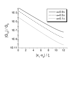
Figure 4: The absolute value of $G_{12}$ at $T=0$ as a function of the distance between the barriers $|x_{2}-x_{1}|$. Similarly to the case $\omega=0$ the dependence $|G_{12}|\sim\exp(-|x_{1}-x_{2}|/\xi)$ is observed at subgap frequencies. Here we set $V_{2}=0$, $L=20\xi$ and $x_{1}=7\xi$.

The non-local conductance $G_{12}$ at zero dc bias $V_{2}=0$ and different frequencies $\omega$ of an ac field is displayed in Fig. 3. We again observe that at $T=0$ and at frequencies $\omega$ below the superconducting gap $\Delta$ CAR dominates over EC thus turning the real part part of the non-local conductance negative, see Fig. 3a. This picture gets modified at non-zero $T$, in which case EC contribution turns out to exceed that of CAR at sufficiently small $\omega$, though at higher frequencies CAR can still win over EC, cf. Fig. 3c. We also observe that a peak in the real part of the non-local conductance develops at low frequencies and non-zero $T$. The height of this peak is essentially determined by elastic cotunneling and is defined by a simple combination $G_{0}[1-\tanh\Delta/2T]$ (see Eq. (44)), while its width is roughly proportional to the Thouless energy $D_{S}/|x_{1}-x_{2}|^{2}$ and slightly increases with temperature. At high enough temperatures $T>\Delta(T)$ all singularities in the non-local conductance are smeared and essentially disappear.

At any subgap frequency $|\omega|<2\Delta$ the zero bias non-local conductance decays exponentially with the distance between the barriers. Similarly to the case $\omega=0$ for all $|\omega|<\Delta$ we find $|G_{12}|\sim\exp(-|x_{1}-x_{2}|/\xi)$ as it is illustrated in Fig. 4.

4 Non-linear response

Finally let us turn to the non-linear non-local response. Choosing the bias voltage in the form $V_{2}(t)=V_{2}+\delta V_{2}\cos\omega t$ we reconstruct the phase

$$\varphi_{2}(t)=eV_{2}t+\frac{e\delta V_{2}}{\omega}\sin\omega t.$$

Substituting this function into Eq. (37) and averaging $\sin[\varphi_{2}(t_{1})-\varphi_{2}(t_{2})]$ over time, we obtain

$$\overline{\sin[\varphi_{2}(t_{1})-\varphi_{2}(t_{2})]}=\sin[eV_{2}(t_{1}-t_{2})]\bigg{[}J_{0}^{2}\left(\frac{e\delta V_{2}}{\omega}\right)$$

$$+2\sum_{n=1}^{\infty}J_{n}^{2}\left(\frac{e\delta V_{2}}{\omega}\right)\cos[n\omega(t_{1}-t_{2})]\bigg{]},$$ (45)

where $J_{n}(x)$ are the Bessel functions. Then the non-local differential conductance takes the form

$$-\frac{\partial I_{12}}{\partial V_{2}}=J_{0}^{2}\left(\frac{e\delta V_{2}}{\omega}\right)G_{12}(0,V_{2})+\sum_{n=1}^{\infty}J_{n}^{2}\left(\frac{e\delta V_{2}}{\omega}\right)$$

$$\times\,\left[G_{12}\left(0,V_{2}+\frac{n\omega}{e}\right)+G_{12}\left(0,V_{2}-\frac{n\omega}{e}\right)\right].$$ (46)

Here $G_{12}(0,V_{2})$ is non-local conductance defined in Eq. (44). We observe that the non-local differential conductance (46) does not change its sign and for non-zero $\omega$ remains positive at all values of the bias voltage $V_{2}$.

5 Concluding remarks

Our analysis of the effect of an external ac bias on non-local electron transport in multi-terminal NSN structures revealed a number of interesting features which can be tested in future experiments. It turns out that in the presence of an ac field exact cancellation between zero-temperature EC and CAR contributions to the non-local current is lifted already in the lowest order in the transmissions of NS interfaces. In the presence of ac bias – unlike in its absence – the conductance $G_{12}$ (39) is not anymore proportional to the density of states in the S-metal (which vanishes at subgap energies thus explaining the cancellation [7]). Hence, no cancellation between EC and CAR contributions to $G_{12}(\omega)$ should be expected. Considering these two contributions separately, we observe that both EC and CAR processes get enhanced by external radiation, however the subtle balance between them is eliminated. As a result, at sufficiently small (typically subgap) frequencies $\omega$ of the external ac signal the non-local conductance of the NSN device $G_{12}$ turns negative implying that CAR contribution wins over that of EC. Although our present analysis was carried out for diffusive structures our key conclusions should also apply in the (quasi-)ballistic limit.

The behavior described above can be realized in multi-terminal NSN structures either under direct application of an ac bias or if the geometry is such that an ac Josephson effect can occur somewhere in the system in the presence of a dc voltage bias. This can be the case, e.g. if a weak link (such as a pinhole or constriction) is occasionally formed between different superconducting terminals. In this case ac Josephson generation may occur under dc bias effectively playing a role of an ac signal analyzed in our work.

We also note that our results – though indirectly – could also be of some relevance to the effect of electron-electron interactions on the non-local properties of NSN devices. Indeed, it is well known that this effect can generally be described by (quantum) electromagnetic fields which mediate electron-electron interactions. In this respect photon-assisted violation of balance between EC and CAR (in favor of the latter process) considered here might give a clue in which way Coulomb interaction could be responsible for the negative non-local conductance observed in recent experiments. However, a more elaborate calculation is necessary to properly account for an interplay between disorder and electron-electron interactions in multi-terminal NSN structures. This calculation will be published elsewhere.

References

• [1] \NameByers J.M. Flatte M.E. \REVIEWPhys. Rev. Lett. 741995306.
• [2] \NameDeutscher G. Feinberg D. \REVIEWAppl. Phys. Lett.762000487.
• [3] \NameBeckmann D., Weber H.B., v. LΓΆhneysen H. \REVIEWPhys. Rev. Lett.932004197003; \NameBeckmann D. v. LΓΆhneysen H. \REVIEWAppl. Phys. A892007603.
• [4] \NameRusso S., Kroug M., Klapwijk T.M., Morpurgo A.F. \REVIEWPhys. Rev. Lett.952005027002.
• [5] \NameCadden-Zimansky P. Chandrasekhar V. \REVIEWPhys. Rev. Lett.972006237003; P. \NameCadden-Zimansky P., Jiang Z., Chandrasekhar V. \REVIEWNew J. Phys.92007116.
• [6] \NameKleine A., Baumgartner A., Trbovic J., SchΓΆnenberger C. arXiv:0812.3553.
• [7] \NameFalci G., Feinberg D., Hekking F.W.J. \REVIEWEurophys. Lett.542001255.
• [8] \NameLesovik G.B., Martin T., Blatter G. \REVIEWEur. Phys. J. B242001287.
• [9] \NameMelin R. Feinberg D. \REVIEWPhys. Rev. B702004174509.
• [10] \NameBrinkman A. Golubov A.A. \REVIEWPhys. Rev. B742006214512.
• [11] \NameMorten J.P., Brataas A., Belzig W. \REVIEWPhys. Rev. B742006214510.
• [12] \NameKalenkov M.S. Zaikin A.D. \REVIEWPhys. Rev. B752007172503.
• [13] \NameGolubev D.S. Zaikin A.D. \REVIEWPhys. Rev. B762007184510.
• [14] \NameKalenkov M.S. Zaikin A.D. \REVIEWPhys. Rev. B762007224506; \REVIEWPhysica E402007147.
• [15] \NameLevy Yeyati A., Bergeret F.S., Martin-Rodero A., Klapwijk T.M. \REVIEWNat. Phys.32007455.
• [16] \NameKalenkov M.S. Zaikin A.D. \REVIEWPis’ma v ZhETF872008166 [\REVIEWJETP Lett.872008140].
• [17] \NameMorten J.P., Huertas-Hernando D., Belzig W.,Brataas A. \REVIEWPhys. Rev. B782008224515.
• [18] \NameFutterer D., Governale M., Pala M.G., KΓΆnig J. \REVIEWPhys. Rev. B792009054505.
• [19] \NameMelin R., Bergeret F., Levy Yeyati A. arXiv:0811.3874v2.
• [20] \NameZaikin A.D. \REVIEWPhyica B2031994255.
• [21] \NameHuck A., Hekking F.W.J., Kramer B. \REVIEWEurophys. Lett.411998201.
• [22] \NameGalaktionov A.V. Zaikin A.D. \REVIEWPhys. Rev. B732006184522.
• [23] \NameBlonder G.E., Tinkham M., Klapwijk T.M. \REVIEWPhys. Rev. B2519824515.
• [24] \NameVolkov A.F., Zaitsev A.V., Klapwijk T.M. \REVIEWPhysica C210199321.
• [25] \NameHekking F.W.J. Nazarov Yu.V. \REVIEWPhys. Rev. Lett.7119931625.