A multimode model for projective photon-counting measurements

Abstract

We present a general model to account for the multimode nature of the quantum electromagnetic field in projective photon-counting measurements. We focus on photon-subtraction experiments, where non-gaussian states are produced conditionally. These are useful states for continuous-variable quantum information processing. We present a general method called mode reduction that reduces the multimode model to an effective two-mode problem. We apply this method to a multimode model describing broadband parametric downconversion, thereby improving the analysis of existing experimental results. The main improvement is that spatial and frequency filters before the photon detector are taken into account explicitly. We find excellent agreement with previously published experimental results, using fewer free parameters than before, and discuss the implications of our analysis for the optimized production of states with negative Wigner functions.

I Introduction

The ability to prepare and measure specific quantum states of the light is the keystone of many quantum information processing (QIP) protocols. These states can be described either with discrete variables in terms of photons, or with continuous variables in terms of waves. In the latter case, the physical quantities of interest are the amplitude and the phase of the light wave, or their Cartesian counterparts called quadratures $\widehat{x}$ and $\widehat{p}$. A very convenient representation of the quantum state is then provided by the Wigner function $W(x,p)$, which corresponds to a quasi-probability distribution of the quadratures, ‘quasi-’ because $W$ may assume negative values.

An important task for QIP is the ability to undo effects of decoherence by ‘distillation’: to obtain a single quantum state that is more pure from two or more copies that have undergone decoherence. Since states of light with gaussian Wigner functions cannot be distilled with gaussian operations Eisert2002a ; Giedke , one is left with two strategies: either to distill gaussian states with non-gaussian operations, or to distill non-gaussian states with gaussian operations Browne . This paper is a contribution to the latter strategy, and focuses on the preparation of the non-gaussian states rather than on their distillation.

The negativity of the Wigner function is a standard figure of merit, quantifying at the same time how non-gaussian and how non-classical a quantum state is Kim2005a ; Biswas2007a . One way of obtaining non-gausian states is by conditional photon-counting measurements, as first proposed by Dakna et al. Dakna1997a . It was soon realized that such conditional measurements can improve quantum teleportation of continuous variables Opatrny2000a . In recent years, several experiments Lvovsky ; WengerCond ; Ourjoumtsev2006a ; Ourjoumtsev2006b ; Wakui ; Neergaard ; Ourjoumtsev2006c ; Parigi2007a combining continuous- and discrete-variable tools allowed for preparing and observing quantum states of free-propagating light with negative Wigner functions Kim2008a .

Many of these experiments are based on the use of a squeezed vacuum produced by parametric fluorescence, which involves many optical modes Avenhaus . This multimode nature is exhibited in both continuous-wave (CW) operation, using optical parametric oscillators (OPO) below threshold Suzuki ; Molmer , and in pulsed experiments with a single-pass high amplification. In order to make accurate predictions, it is therefore crucial to develop multimode theoretical models. This was done in Suzuki ; Molmer ; Nielsen2007a ; Nielsen2007b for setups using an OPO, and in prl ; Aichele for pulsed $1$-photon Fock state tomography in a case of very low squeezing, when Fock states expansion are limited to $1$ photon only. However, these models do not fully account for all phenomena linked to the non-constant space and time profiles of the modes under study, the spatial pulse profile in the transverse direction for example, and they especially do not account for gain-induced distortions in the parametric amplification process LaPorta . As we will see later on, these phenomena are one main signature of this multimode nature, and are critical in the case of single-pass pulsed experiments.

In this paper we propose an alternative general framework to describe the generation of squeezed light, with a twofold goal: first, to introduce a method that reduces a multimode model to an effective two-mode description. Second, to show that a specific spatio-temporal multimode model for photon-subtraction experiments and our mode-reduction analysis thereof give an improved understanding of state-of-the-art photon-subtraction experiments.

In Sec. II we show how to reduce a multi-mode model to an effective two-mode model. This mode-reduction procedure is then applied in Sec. III to give an improved analysis of the photon-subtraction experiments of Ref. Ourjoumtsev2006a . We discuss the method and its application and conclude in Sec. IV. Some technicalities are deferred to two Appendices.

II Reduction of multimode model

II.1 General multimode model

As a starting point we have a complete set of spatial, temporal, or spatio-temporal optical modes, in terms of which the light propagation can be described. The modes have field operators $\hat{\text{a}}_{j}$ and $\hat{\text{a}}_{j}^{{\dagger}}$ with bosonic commutation relations $[\hat{\text{a}}_{j},\hat{\text{a}}_{k}^{\dagger}]=\delta_{jk}$. The $\hat{\text{a}}_{j}$ may also stand for continuous operators like $\hat{\text{a}}(t)$, where $t$ is time, with commutation relation $[\hat{\text{a}}(t),\hat{\text{a}}^{{\dagger}}(t^{\prime})]=\delta(t-t^{\prime})$, in which case sums over modes are to be replaced with integrals. To simplify the notation even further, we introduce $\vec{\hat{\text{a}}}$, the column vector of all the $\hat{\text{a}}_{j}$. Similarly $\vec{\hat{\text{a}}}^{\dagger}$ is the row vector which has operators $\hat{\text{a}}_{j}^{\dagger}$ as components. We shall also need the row vector $\vec{\hat{\text{a}}}^{T}$ and the column vector $\vec{\hat{\text{a}}}^{*}=\vec{\hat{\text{a}}}^{{\dagger}T}$. Similar notation will be used for other vectors.

In this section we consider a general unitary transformation $U$ in which output quadratures linearly depend on input quadratures, thus preserving the gaussian nature of the quantum fields. In fact, the only non-gaussian operation will be the projective measurement, corresponding to a detection event in a subset of the output modes by an avalanche photodiode (APD), see Figure 1.

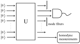
Figure 1: Projective photon-counting measurement: in our model we assume that we start with a multimode vacuum input state which is subject to a general multimode Bogoliubov transform $U$. After the transformation a few modes are filtered out and result in a detection event in the avalanche photodiode (APD). Such a detection event in the APD prepares a state in the single mode which is mode analyzed by homodyne detection.

We will assume the evolution operator $U$ in Fig. 1 to be a Bogoliubov transformation, where the output field operators depend linearly on the input ones:

$$\qquad\vec{\hat{\text{a}}}_{\rm out}=U^{\dagger}\vec{\hat{\text{a}}}\,U=u\,\vec{\hat{\text{a}}}+v\,\vec{\hat{\text{a}}}^{*},$$ (1)

where $u$ and $v$ are two matrices which satisfy

$$uu^{\dagger}-vv^{\dagger} = u^{\dagger}u-v^{\dagger}v=1,$$ (2a)

$$uv^{T}-vu^{T} = 0,$$ (2b)

whereby the commutation relations of the field operators are preserved. The output state of the light can be characterized by doing homodyne measurements on a normalized mode described by $\vec{\psi}_{h}$, which has the mode operator

$$\hat{a}_{h}=\vec{\psi}_{h}^{\dagger}\,\vec{\hat{\text{a}}}.$$ (3)

This mode can be defined as the mode that perfectly matches the local oscillator of the homodyne detector. After the Bogoliubov transform (1) it is described by

$$\hat{a}_{h,{\rm out}}=U^{\dagger}\hat{a}_{h}U=\vec{\psi}_{h}^{\dagger}(u\,\vec{\hat{\text{a}}}+v\,\vec{\hat{\text{a}}}^{*}).$$ (4)

Without conditioning upon photon detection, and since the gaussian nature of the initial vacuum state is preserved by the Bogoliubov transform, the homodyne measurements will show gaussian Wigner functions corresponding to squeezed vacuum states of light.

The point is now how to describe the output state conditional upon detection of a photon by the APD, which is a projective measurement. Analogous to the homodyne detection, we assume the photon detection mode $j$ to be described by a normalized state $\phi_{d}(j)$, with corresponding field operator

$$\hat{a}_{d}(j)=\vec{\phi}_{d}^{\dagger}(j)\vec{\hat{\text{a}}}.$$ (5)

After the time evolution described by Eq. (1), the output at the photon detector becomes:

$$\hat{a}_{d,{\rm out}}(j)=U^{\dagger}\hat{a}_{d}(j)U=\vec{\phi}_{d}^{\dagger}(j)(u\,\vec{\hat{\text{a}}}+v\,\vec{\hat{\text{a}}}^{*}).$$ (6)

If we only know that a photon has been detected but not in which detection mode, then we should average the conditional output state over all these detection modes, as is shown in more detail below.

At this point we have a multimode output state that in principle we can update given the detection of a photon in the detector $j$. In practice it is convenient to first simplify the multimode expressions (4) and (6).

II.2 Mode reduction

The first and central step in the mode-reduction procedure is to rewrite the homodyne mode Eq. (4) in the form

$$\hat{a}_{h,{\rm out}}=\eta\,\hat{a}_{0}+\alpha\,\hat{a}_{0}^{\dagger}+\beta\,\hat{a}_{1}^{\dagger},$$ (7)

in terms of new mode operators $a_{0,1}^{({\dagger})}$ with standard commutation relations. The coefficients $\eta,\alpha$, and $\beta$ in Eq. (7) are found as follows. Besides having standard commutations, $\hat{a}_{0}$ and $\hat{a}_{1}$ in Eq. (7) should annihilate the vacuum state, so that $\hat{a}_{0}$ must contain all annihilation operators in Eq. (4):

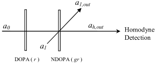
Figure 2: Equivalent model for the Bogoliubov transform U: a perfect single-mode degenerate optical parametric amplifier (DOPA) with squeezing parameter $r$ is followed by a perfect non-degenerate optical parametric amplifier (NDOPA) with squeezing parameter $gr$.

$$\eta\,\hat{a}_{0}=\vec{\psi}_{h}^{\dagger}u\,\vec{\hat{\text{a}}},$$ (8)

with $\eta$ fixed up to a phase factor by $[\hat{a}_{0},\hat{a}_{0}^{\dagger}]=1$. We choose $\eta$ to be real-valued and positive so that

$$\eta=\sqrt{\vec{\psi}_{h}^{\dagger}uu^{\dagger}\vec{\psi}_{h}}.$$ (9)

Furthermore, from $[\hat{a}_{0},\hat{a}_{1}^{{\dagger}}]=0$ it follows that

$$\alpha=[\hat{a}_{0},\hat{a}_{h,{\rm out}}]=\frac{1}{\eta}\vec{\psi}_{h}^{\dagger}\,u\,v^{T}\,\vec{\psi}_{h}^{*}.$$ (10)

A complex value for $\alpha$ can be removed with a redefinition of the phase of the homodyne mode, which just means that we can assume that the state is squeezed in the $x$ or $p$ direction. Finally, $\beta$ can be found from the fact that $\hat{a}_{h,{\rm out}}$ and $\hat{a}_{h,{\rm out}}^{\dagger}$ have commutator one, as have $\hat{a}_{1}$ and $\hat{a}_{1}^{\dagger}$:

$$\beta=\sqrt{\eta^{2}-\alpha^{2}-1}.$$ (11)

Here again we used the freedom to choose $\beta$ real-valued and nonnegative. This completes the mathematics of the mode reduction of the multimode homodyning signal.

The physical argument that two and only two modes should remain goes as follows. The squeezed vacuum after the Bogoliubov transform can only be a centered gaussian state, hence it is fully described by only the variances $V_{x}$ and $V_{p}$. The squeezed vacuum output can therefore be modeled Gardiner2000a ; Wenger by a perfect single-mode degenerate optical parametric amplifier (DOPA) with squeezing parameter $r$, followed by a perfect non-degenerate optical parametric amplifier (NDOPA) with squeezing parameter $gr$, as presented in Figure 2. This is a two-mode model, with a Hilbert space $\mathcal{H}_{2}$. The values of the parameters $r$ and $g$ can be deduced from the two independent coefficients in Eqs. (9-11), using:

$$\eta = \cosh(r)\cosh(gr)$$ (12a)

$$\alpha = \sinh(r)\cosh(gr)$$ (12b)

$$\beta = \sinh(gr).$$ (12c)

A related squeezing parameter that we will also use in the following is $s\equiv\exp(-2r)$.

II.3 Conditioning upon photon detection

We now condition upon the measurement of a click in the photon detector (APD). We assume to be in the limit that the average number of photons per pulse entering the photon detector is much less than one. Then a single click in the detector corresponds to the detection of a single photon.

One can make a reduced-mode description of the photon detection operator $\hat{a}_{d,{\rm out}}(j)$ of Eq. (5), analogous to Eq. (7). The operator $\hat{a}_{d,{\rm out}}(j)$ can be expanded into a part acting on $\mathcal{H}_{2}$, plus a component $\hat{a}_{d\perp}(j)$ acting on the complementary space $\mathcal{H}_{\perp}$ orthogonal to $\mathcal{H}_{2}$:

$$\hat{a}_{d,{\rm out}}(j)=\gamma_{j}\hat{a}_{0}^{\dagger}+\delta_{j}\hat{a}_{1}^{\dagger}+\epsilon_{j}\hat{a}_{0}+\kappa_{j}\hat{a}_{1}+\hat{a}_{d\perp}(j).$$ (13)

Note that $\hat{a}_{d\perp}(j)$ on the right-hand side contains all the terms acting on $\mathcal{H}_{\perp}$, including creation operators. The coefficients in (13) can again be found by taking commutators, for example:

$$\gamma_{j} = [\hat{a}_{0},\hat{a}_{d,{\rm out}}(j)]=\frac{1}{\eta}\vec{\psi}_{h}^{\dagger}\,u\,v^{T}\,\vec{\phi}_{d}^{*}(j)$$ (14a)

$$\delta_{j} = [\hat{a}_{1},\hat{a}_{d,{\rm out}}(j)]=\frac{1}{\beta^{*}}[\vec{\phi}_{d}^{\dagger}(j)\,v\,v^{\dagger}\,\vec{\psi}_{h}-\alpha^{*}\gamma_{j}].$$ (14b)

In general, a click recorded in the APD corresponds to the measurement of at least one photon. In the limit of low detection probability, the action of the detection is the subtraction of a single photon. Note that this assumption is practically always obeyed if the parameter $j$ is in a continuum (like in the case of spectral filtering), since the probability to have two photons exactly in the same mode is then negligible. Henceforth we assume to be in this limit. In the Heisenberg picture, a photon detection then corresponds to the application of the operator $\hat{a}_{d,{\rm out}}(j)$ to the initial state (i.e. to the vacuum state), followed by the normalization of the result:

$$|\Psi(j)\rangle=P_{j}^{-1/2}\hat{a}_{d,{\rm out}}(j)|0\rangle$$ (15)

where $P_{j}$ is the detection probability for the mode $j$:

$$P_{j} = \langle 0|\hat{a}_{d,{\rm out}}^{\dagger}(j)\hat{a}_{d,{\rm out}}(j)|0\rangle$$

$$= \langle 0|\hat{a}_{d\perp}^{\dagger}(j)\hat{a}_{d\perp}(j)|0\rangle+|\gamma_{j}|^{2}+|\delta_{j}|^{2}$$

$$= \overrightarrow{\phi}_{d}^{\dagger}(j)vv^{\dagger}\overrightarrow{\phi}_{d}(j).$$

Below we will use that the vacuum expectation value of $\hat{n}_{d\perp}(j)=\hat{a}_{d\perp}^{\dagger}(j)\hat{a}_{d\perp}(j)$ can be expressed as $P_{j}-|\gamma_{j}|^{2}-|\delta_{j}|^{2}$.

Before continuing, it can be instructive to recall the concision allowed by the Heisenberg picture. In a single-mode problem, a photon-subtracted squeezed state is equivalent to a squeezed single-photon state: this case corresponds to the simple Bogoliubov transform $\hat{a}_{\rm out}=\cosh(r)\hat{a}_{\rm in}+\sinh(r)\hat{a}^{\dagger}_{\rm in}$, which directly gives a pure $1$-photon state (after normalization) when applied to the vacuum. As the states do not evolve in the Heisenberg picture, they all can be considered as ‘input’ states; but when measured using output quadratures, this $1$-photon state will appear to be squeezed.

We are going to use the same approach in the multimode case. One can first note that the conditioned state $|\Psi(j)\rangle$ in Eq. (15) is already a $1$-photon state. This state, however, does not belong to $\mathcal{H}_{2}$ only, so that measurements output are not so obvious to compute. In fact, we are solely interested in expectation values $\langle g(a_{h,\rm out},a_{h,\rm out}^{{\dagger}})\rangle$ of operators describing the output that is measured in the homodyne detector. Such expectation values can be written as

$$\langle g(a_{h,\rm out},a_{h,\rm out}^{{\dagger}})\rangle = \langle\psi_{j}|\,g(\hat{a}_{h,{\rm out}},\hat{a}_{h,{\rm out}}^{{\dagger}})\,|\psi_{j}\rangle$$ (17a)

$$= \mbox{Tr}\{g(\hat{a}_{h,{\rm out}},\hat{a}_{h,{\rm out}}^{{\dagger}})|\psi_{j}\rangle\langle\psi_{j}|\}.~{}~{}~{}~{}~{}~{}$$ (17b)

In Eq. (17b), the trace can be separated into a trace over $\mathcal{H}_{2}$ and a trace over $\mathcal{H}_{\perp}$, and the latter does not act on the function $g(\hat{a}_{h,{\rm out}},\hat{a}_{h,{\rm out}}^{{\dagger}})$, whose expectation value is then:

$$= \mbox{Tr}_{2}\{g(\hat{a}_{h,{\rm out}},\hat{a}_{h,{\rm out}}^{{\dagger}})\mbox{Tr}_{\perp}|\psi_{j}\rangle\langle\psi_{j}|\}$$ (18a)

$$= \mbox{Tr}_{2}\{g(\hat{a}_{h,{\rm out}},\hat{a}_{h,{\rm out}}^{{\dagger}})\rho_{j}\}$$ (18b)

All quantities of interest can therefore be deduced from the input state reduced density matrix $\rho_{j}$, acting in $\mathcal{H}_{2}$, and the crucial advantage of mode reduction is to allow a simple expression for this matrix: Writing $|0\rangle=|00\rangle\otimes|0\rangle_{\perp}$, where $|00\rangle$ and $|0\rangle_{\perp}$ are the ground states of $\mathcal{H}_{2}$ and $\mathcal{H}_{\perp}$, respectively, and using Eqs. (13,15), we directly obtain:

$$\rho_{j} = \mbox{Tr}_{\perp}|\psi_{j}\rangle\langle\psi_{j}|$$

$$= (1-\xi_{j})\,|00\rangle\langle 00|+\xi_{j}\,\hat{a}_{\theta}^{\dagger}(j)|00\rangle\langle 00|\hat{a}_{\theta}(j),$$

in terms of the modal purity

$$\xi_{j}=\frac{|\gamma_{j}|^{2}+|\delta_{j}|^{2}}{P_{j}},$$ (20)

and where

$$\hat{a}^{\dagger}_{\theta}(j)=\cos\theta_{j}\hat{a}_{0}^{\dagger}+\sin\theta_{j}\hat{a}_{1}^{\dagger},\quad\mbox{with}\;\;\tan\theta_{j}=\delta_{j}/\gamma_{j}$$ (21)

is an operator that creates a single photon in a superposition of mode 0 and mode 1. The state (II.3) produced from a detection event in mode $j$ is a mixed state, mixing vacuum and a single-photon state with weight $\xi_{j}$. Without conditioning or in the limit $\xi_{j}\rightarrow 0$, we have $\rho_{j}=|00\rangle\langle 00|$.

II.4 Wigner functions

Squeezed vacuum.— Before determining the output Wigner function corresponding to the conditional state (II.3), it is instructive to first determine the Wigner function of the output state in the simplest experimental situation, where we ignore the photon detector. The input state is then $\rho=|00\rangle\langle 00|$. We will make use of the standard Wigner functions of the vacuum $W_{0}(x,p)=\exp(-r^{2})/\pi$ and of single-photon states $W_{1}(x,p)=(2r^{2}-1)\exp(-r^{2})/\pi$, both with $r^{2}=x^{2}+p^{2}$. Clearly, $W[\rho](x_{0},p_{0};x_{1},p_{1})$ equals $W_{0}(x_{0},p_{0})W_{0}(x_{1},p_{1})$.

In order to obtain the output Wigner function for the homodyne mode, we wish to express $W[\rho]$ as a function of $x_{h,\rm out}$, $p_{h,\rm out}$ (defined from the output homodyne mode $\hat{a}_{h,\rm out}$ given by Eq. (7)). This requires the introduction of another mode $\hat{a}_{1,{\rm out}}$ orthogonal to $a_{h,{\rm out}}$, so that the transformation $(\hat{a}_{0},\hat{a}_{1})\rightarrow(\hat{a}_{h,\rm out},\hat{a}_{1,\rm out})$ is symplectic (i.e. commutation relations are preserved). Using the model of Fig. 2, one can choose $\hat{a}_{1,{\rm out}}$ of the form:

$$\hat{a}_{1,{\rm out}}=\beta\,\frac{\alpha\,\hat{a}_{0}+\eta\,\hat{a}_{0}^{\dagger}}{\sqrt{1+\beta^{2}}}+\sqrt{1+\beta^{2}}\,\hat{a}_{1}.$$ (22)

This form is by no means unique, but this does not pose a problem since mode $1_{\rm out}$ will eventually be integrated out. One can now invert the relations (7,22), thereby expressing $x_{0,1},p_{0,1}$ as a function of $x_{h,{\rm out}},p_{h,{\rm out}},x_{1,{\rm out}}$, and $p_{1,{\rm out}}$. After tracing over mode $1_{\rm out}$, which amounts to integrating over $x_{1,{\rm out}}$ and $p_{1,{\rm out}}$, we find the output signal entering the homodyne detector to be a squeezed vacuum state with a gaussian Wigner function

$$W_{0,{\rm sqz}}(x,p)=\frac{1}{\pi\sqrt{V_{x}V_{p}}}\exp\left(-\frac{x^{2}}{V_{x}}-\frac{p^{2}}{V_{p}}\right),$$ (23)

where $x$ and $p$ stand for $x_{h,{\rm out}}$ and $p_{h,{\rm out}}$ and with variances

$$V_{x} = (\eta+\alpha)^{2}+\beta^{2}$$ (24a)

$$V_{p} = (\eta-\alpha)^{2}+\beta^{2}.$$ (24b)

We can now invert Eq. (24) and rewrite the three mode-reduction parameters $\alpha,\eta$, and $\beta$ in Eq. (7) in terms of the variances, giving:

$$\eta = \frac{V_{p}+V_{x}+2}{2\sqrt{V_{x}+V_{p}+2}},$$ (25a)

$$\alpha = \frac{V_{x}-V_{p}}{2\sqrt{V_{x}+V_{p}+2}},$$ (25b)

$$\beta = \frac{2\sqrt{V_{x}V_{p}-1}}{2\sqrt{V_{x}+V_{p}+2}}.$$ (25c)

In the following, we will keep writing $\alpha,\eta$, and $\beta$ to shorten notation. It should be kept in mind, however, that Eq. (25) directly expresses these parameters in terms of the measurable variances $V_{x,p}$ of the squeezed vacuum. In particular, $\beta$ vanishes for minimal-uncertainty states.

Notice also that the parametrization for the mode-reduction parameters (25) is equivalent to the one in Eq. (12) in terms of squeezing parameters $r$ and $g$. Thus $r$ and $g$ can be expressed in terms of the variances $V_{x,p}$, and vice versa.

Photon-subtracted squeezed vacuum.— As for the squeezed vacuum, we now calculate the Wigner function for the photon-subtracted squeezed vacuum, starting with the initial state (II.3). The mode (21) has a one-photon excitation in state (II.3). The orthogonal mode with creation operator $\hat{a}_{\theta+\pi/2}^{{\dagger}}(j)$ is not excited. Hence the Wigner function corresponding to the state (II.3) is

$$W(x_{0},p_{0};x_{1},p_{1}) = (1-\xi_{j})\,W_{0}(x_{0},p_{0})W_{0}(x_{1},p_{1})$$

$$+ \xi_{j}\,W_{1}(x_{\theta_{j}},p_{\theta_{j}})W_{0}(x_{\theta_{j}+\pi/2},p_{\theta_{j}+\pi/2}).$$

Note that in this expression, quadratures $x_{\theta_{j},\theta_{j}+\pi/2}$, $p_{\theta_{j},\theta_{j}+\pi/2}$ can be easily expressed as functions of quadratures $x_{0,1},p_{0,1}$ using (21). As before, the Wigner function for the output signal is found by using the symplectic transformation defined by Eqs. (7) and (22). By tracing again over the mode $1_{\rm out}$, we obtain (see appendix A)

$$W_{j}(x,p)=\left(C_{j}+2A_{j}\frac{x^{2}}{V^{2}_{x}}+2B_{j}\frac{p^{2}}{V^{2}_{p}}+D_{j}\frac{xp}{V_{x}V_{p}}\right)W_{0,{\rm sqz}}.$$ (27)

The constants in this Wigner function are given by

$$A_{j} = P_{j}^{-1}|\gamma_{j}(\eta+\alpha)+\delta_{j}\beta|^{2},$$ (28a)

$$B_{j} = P_{j}^{-1}|\gamma_{j}(\eta-\alpha)-\delta_{j}\beta|^{2},$$ (28b)

$$C_{j} = 1-A_{j}/V_{x}-B_{j}/V_{p},$$ (28c)

$$D_{j} = -8P_{j}^{-1}\mbox{Im}(\gamma^{*}_{j}\delta_{j})\eta\beta.$$ (28d)

Note that the Wigner function (27) of the photon-subtracted squeezed state differs from the Wigner function of the squeezed vacuum $W_{0,{\rm sqz}}(x,p)$ of Eq. (23) only because of the polynomial in $x$ and $p$ between the large brackets. The same quantities $V_{x,p}$ as in Eq. (24) show up, with or without conditioning. Since in general $W(x,p)\geq-\pi^{-1}$ Leonhardt1997a , we find the condition $C_{j}\geq-1$.

Averaged Wigner functions.— Practical detectors do not resolve with infinite precision when and where photons are detected. We should therefore average over all possible microscopic states that agree with the detection record. We assumed in Sec. II.3 that the average number of photons detected per pulse in the APD is much smaller than one. Averaging over unresolved detection events is then equivalent to averaging over single-photon subtraction events.

The Wigner transformation of the density matrix is a linear transformation. Therefore, the averaged Wigner function $\overline{W}(x,p)$ is simply obtained by replacing $A_{j}$…$D_{j}$ in (27) by $\overline{A}$…$\overline{D}$, with the notation

$$\overline{X}=P_{\rm tot}^{-1}\sum_{j}P_{j}X_{j}.$$ (29)

Here $P_{\rm tot}$ is the sum of the probabilities $P_{j}$ of microscopic states that agree with the detection record. From Eq. (28) it follows that averaged quantities $\overline{A}$…$\overline{D}$ involve sums like $\sum_{j}|\gamma_{j}|^{2}$, $\sum_{j}|\delta_{j}|^{2}$ or $\sum_{j}\gamma_{j}^{*}\delta_{j}$; in the following we will write the respective averages as $\overline{|\gamma|^{2}}$, $\overline{|\delta|^{2}}$ or $\overline{\gamma^{*}\delta}$.

The Wigner function (27) of the photon-subtracted state and its detection-averaged version have a very general significance. Before going to Sec. III, devoted to a practical implementation of these results, let us finish with some reflections on the detection modes.

II.5 Detection modes

All the previous results were derived through the use of a set of detection modes $\hat{a}_{d}(j)$. The coefficients entering in the averaged Wigner function $\overline{W}$ involve quantities like $P_{\rm tot}$, $\overline{|\gamma|^{2}}$, $\overline{|\delta|^{2}}$ or $\overline{\gamma^{*}\delta}$, in which the detection operators only appear through their projection operator:

$$\Pi=\sum_{j}\vec{\phi}_{d}(j)\vec{\phi}_{d}^{\dagger}(j).$$ (30)

Hence one would find the same predicted averages if one would employ a different set of detection modes that has the same associated projector. This projector describes how the setup filters the signal before it enters the photon detector. For example, a time-domain filtering system will be described by $\Pi=\Pi_{T}$, where $\Pi_{T}$ can be written in terms of a set of modes $\hat{\text{a}}(t)$ that are labeled by the time $t$:

$$\Pi_{T}(t,t^{\prime})=T(t)\delta(t-t^{\prime}),$$ (31)

where $T(t)=1$ when the APD is switched on, and $T(t)=0$ otherwise. To give another important example, a spectral slit can be described with a set of modes $\hat{\text{a}}(\omega)$ with an associated projector

$$\Pi_{\Omega}(\omega,\omega^{\prime})=T(\omega)\delta(\omega-\omega^{\prime}),$$ (32)

where $T(\omega)=0$ if the frequency $\omega$ is filtered out, and $T(\omega)=1$ otherwise.

Above we have assumed that the filtering of the signal after its production in the DOPA was included in the Bogoliubov transform $U$. Below we will give an alternative description, in which $U$ is separated into the transformation due to the production of the squeezed light in the DOPA, and the subsequent filtering before detection. This alternative description will enable a more straightforward comparison with the empirical model in Sec. III.

So, instead of the input-output transform Eq. (6) for the photon detection operator, we now write

$$\hat{a}_{d,{\rm out}}(j)=\vec{\phi}_{d}^{\dagger}(j)u_{f}(u\,\vec{\hat{\text{a}}}+v\,\vec{\hat{\text{a}}}^{*}),$$ (33)

where the Bogoliubov matrix $u_{f}$ accounts for filters (as the filters are passive, we have $v_{f}=0$); this matrix $u_{f}$ is of course unitary, even if the filters can present losses. In fact, losses will be modeled using beamsplitters, where the lost energy is reflected into auxiliary non-relevant modes. These modes do not interact with the rest of the experiment (i.e. they are unaffected by Bogoliubov transform $u,v$) and will not reach the APD. But all the other modes, referred to as relevant modes, should be considered as detection modes, and we then have:

$$\sum_{j}\vec{\phi}_{d}(j)\vec{\phi}_{d}^{\dagger}(j)=\Pi_{r},$$ (34)

where $\Pi_{r}$ is the projector onto the subspace of relevant modes. Let $\overline{\Pi}_{r}$ be the projector on the non-relevant modes. As the latter are unaffected by the transform $u,v$, we have $\overline{\Pi}_{r}(u\,\vec{\hat{\text{a}}}+v\,\vec{\hat{\text{a}}}^{*})=\overline{\Pi}_{r}\vec{\hat{\text{a}}}$. Inserting the relation $\Pi_{r}+\overline{\Pi}_{r}=\openone$ into (33) then leads to

$$\hat{a}_{d,{\rm out}}(j)=\vec{\phi}_{d}^{\dagger}(j)u_{f}\Pi_{r}(u\,\vec{\hat{\text{a}}}+v\,\vec{\hat{\text{a}}}^{*})+\vec{\phi}_{d}^{\dagger}(j)u_{f}\overline{\Pi}_{r}\vec{\hat{\text{a}}}.$$ (35)

Here the last term on the right annihilates vacuum, and commutes with annihilation operators like $\hat{a}_{0}$ or $\hat{a}_{1}$: this term will add no contribution to the results of the previous subsection. The only change therefore consists in the substitution $\vec{\phi}\rightarrow\Pi_{r}u_{f}^{\dagger}\vec{\phi}$, so that the operator $\Pi$ in Eq. (30) should be replaced by

$$\Pi^{\prime}=\Pi_{r}u_{f}^{\dagger}\sum_{j}\vec{\phi}_{d}(j)\vec{\phi}_{d}^{\dagger}(j)u_{f}\Pi_{r}=F^{\dagger}F,$$ (36)

where $F=\Pi_{r}u_{f}\Pi_{r}$ and where we have used standard properties of projection operators ($\Pi=\Pi^{\dagger}$, $\Pi^{2}=\Pi$). The operator $F$ represents the action of the filters restricted to the subspace of relevant modes. If $F$ is a projector, such as $\Pi_{T}$ of Eq. (31) or $\Pi_{\Omega}$ of Eq. (32), then the effect of $\Pi^{\prime}$ is the same as of $\Pi$ in Eq. (30). This can be easily understood: it is equivalent to say that the filtered modes are blocked, or that they are first redirected into auxiliary modes, and then blocked.

The operator $\Pi^{\prime}$ of Eq. (36) is a more general quantity than $\Pi$ in Eq. (30), however, since $\Pi^{\prime}$ need not be a projection operator. It can for instance account for partial absorption of the modes. In that case, the spectral transmission $T(\omega)$ in Eq. (32) can assume any value between $0$ and $1$, to account for filtering systems more complex than a simple spectral slit.

Furthermore, the above expressions can simply be generalized to situations where several filters are used. For example, if a spectral slit $\Pi_{\Omega}$ is followed by a time-domain filter $\Pi_{T}$, then the above expressions for $F$ and $\Pi^{\prime}$ become $F=\Pi_{T}\Pi_{\Omega}$, leading to $\Pi^{\prime}=\Pi_{\Omega}\Pi_{T}\Pi_{\Omega}$.

III Application

At this stage, we have a complete description of the final state starting from the Bogoliubov transform (1). The results of the previous section are generally valid, since we started with a multimode model that was left unspecified. Our purpose now is to establish a concrete link with the photon-subtraction experiment as described in Ref. Ourjoumtsev2006a , and to improve its analysis.

III.1 Photon subtraction experiment

In the experiment by Ourjoumtsev et al. Ourjoumtsev2006a , pulses of squeezed light are produced. The setup is sketched in Figure 3.

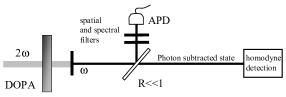
Figure 3: Simplified experimental setup: a squeezed vacuum is generated by a DOPA, where photons of frequency $2\omega$ are transformed into pairs of photons of frequency $\omega$ (in the experiment, the central frequency $\omega_{0}$ corresponds to a central wavelength of about $850~{}nm$). The output signal of the DOPA is sampled by a beam splitter with low reflectivity $R$. If a photon is detected by the APD, then ideally it has been subtracted from the squeezed vacuum.

A squeezed vacuum, produced in a single-pass DOPA (a ${\rm KNbO}_{3}$ crystal) by down-conversion of frequency-doubled femtosecond laser pulses, is sampled by a beam splitter with low reflectivity $R=1-T$. Two mode filters are placed in front of the APD: a spatial mode filter, that consists in a single-mode fiber, and a spectral slit of width $\Omega$. If a photon is detected by the APD, then ideally it has been subtracted from the squeezed vacuum. This subtraction leads to a $1$-photon squeezed state, which is very close to a ‘Schrödinger kitten’ state. Quantum state tomography with a balanced homodyne detector Leonhardt1997a allows the complete reconstruction of this highly non-gaussian quantum state of light.

The Wigner function (27) was derived assuming that the mode reduction was performed on the mode entering the homodyne detector. To relate our results to the empirical model discussed in the next subsection, we here choose to perform the mode reduction to the signal directly after the DOPA. We model the DOPA using the scheme presented in Fig. 2, where the parameters $r$ and $g$ are linked to the Bogoliubov transform through Eqs. (9-12). For the calculation of the modes $\hat{a}_{d,\rm out}(j)$ detected by the APD, the sampling beamsplitter and the mode filters can be separately added to this transform, as explained in Sec. II.5. As stated above, here we chose not to include the sampling beam splitter into the mode reduction. The Wigner function (27) then describes the signal just after the DOPA. We therefore still need to account for this sampling beam splitter between the DOPA and the homodyne detection, as well as for other losses. For example, one usually accounts for imperfections of the homodyne detection by adding a fictitious beam splitter of transmission $\eta_{\rm hom}$ just before the homodyne detection, where $\eta_{\rm hom}$ is the homodyne detection efficiency. Both those beam splitters can be easily implemented by replacing the variances according to:

$$V^{(m)}_{x/p}-1=\eta_{\rm hom}T[V_{x/p}-1].$$ (37)

and by multiplying $A$, $B$ and $D$ by $\eta_{\rm hom}T$. Before going into detailed calculations, let us first recall the empirical model that was proposed in Ref. Ourjoumtsev2006a to account for experimental results.

III.2 Empirical model

It is useful to recall the empirical model proposed in Ref. Ourjoumtsev2006a to explain the experiments, and to see by what assumptions our multimode model reduces to it. The DOPA is again modeled as in Fig. 2, producing the same squeezed vacuum. However, in the empirical model it is assumed that the detected photon is either in the homodyne mode with probability $\xi$, or in an orthogonal mode with probability $(1-\xi)$. In the latter case, the detection event is not correlated with the homodyne measurement, and one simply performs a homodyne measurement on squeezed vacuum.

The output density matrix obtained with the empirical model is similar to our $\rho_{j}$ in Eq. (II.3). In fact, the two would be identical if the detected photon was only due to photons in the mode $\psi_{h}$ or from $\mathcal{H}_{\perp}$. This is in general not the case, however, as there will be an admixture from $\hat{a}_{1,{\rm out}}$ in the photon detection operator. In fact, in order to completely account for the multimode nature of this experiment, the empirical model should be modified in the way depicted on Fig. 4, with the insertion of a beamsplitter of amplitude reflection and transmission coefficients $\rho$ and $\tau$ that allows interference between $\hat{a}_{h,{\rm out}}$ and $\hat{a}_{1,{\rm out}}$. A photon detection event in such a setup can indeed be equivalent to the application of $\hat{a}_{\theta}^{\dagger}(j)$ to the initial vacuum [see Eqs. (II.3,21)], provided

$$\frac{\rho}{\tau}\cosh(r)=\frac{1}{\tan\theta_{j}}-\frac{1}{\tan\theta_{0}},$$ (38)

with $\tan(\theta_{0})=\beta/\alpha$. These angles $\theta_{0}$ and $\theta_{j}$ are mixing angles that fix the probability amplitudes of detection of a photon of mode 0 and of mode 1. Our angle $\theta_{j}$ in general depends both on the squeezing properties of the light source, and on the filtering of the signal before the photon detector, whereas the empirical $\theta_{0}$ only depends on the source. Within a narrow-filter approximation that will be detailed in next subsection, such a setup can also account for averaged quantities (29) with the use of an average angle $\bar{\theta}$ instead of $\theta_{j}$ (see Eq. (54) in the following).

This possibility of interference between the homodyne signal and the $\hat{a}_{1,{\rm out}}$ signal is the crucial difference between the multimode and the empirical models: More interference makes the empirical model worse. The essential assumption of the empirical model is thus that the photon detection operator does not have a contribution from $\hat{a}_{1,{\rm out}}$. Then $\gamma_{j}$ and $\delta_{j}$ could be replaced by $\alpha$ and $\beta$, respectively, according to Eqs. (7) and (13), and the angle $\theta_{j}$ in Eq. (II.3) by $\theta_{0}$ (in which case, according to Eq. (38), the beamsplitter $BS(\rho,\tau)$ in the equivalent model in Fig. 4 can be removed).

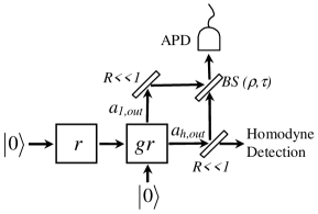
Figure 4: When one applies the mode reduction procedure to the multimode model for photon subtraction as sketched in Fig. 1, the resulting Wigner function is equivalent to the two-mode model depicted in the figure. The DOPA may in general be represented by an ideal single mode DOPA and a two-mode NDOPA as in Fig. 2, and the photon counting is a combination of dark counts as well as a coherent mixture of the two output ports of the NDOPA. Compared to the empirical model developed in Ref. Ourjoumtsev2006a , the only difference is the presence of the beam splitter $BS(\rho,\tau)$ which was not present in the empirical model.

The empirical Wigner function can be easily deduced from Eq. (27) with the above replacements, and has the same form after the replacement of $\bar{A}\cdots\bar{D}$ by $A_{\rm emp}\cdots D_{\rm emp}$. Coefficients $A_{\rm emp}$ and $B_{\rm emp}$ are obtained by multiplying $\bar{A}$, $\bar{B}$ by $\xi/\bar{\xi}$, and replacing $\bar{\gamma}$ and $\bar{\delta}$ by $\alpha$ and $\beta$, respectively. This gives

$$A_{\rm emp}=\xi\frac{(V_{x}-1)^{2}}{V_{x}+V_{p}-2},\qquad B_{\rm emp}=\xi\frac{(V_{p}-1)^{2}}{V_{x}+V_{p}-2}.$$ (39)

The coefficient $C_{\rm emp}$ is given by $C_{\rm emp}=1-A_{\rm emp}/V_{x}-B_{\rm emp}/V_{p}$, and $D_{\rm emp}$ vanishes.

The empirical model produces intuitive results. However, it requires justification. If large spectral slits would be used, then the homodyne mode and many other orthogonal modes would hardly be affected by the slit. If the detected photon could have come from many modes orthogonal to $\psi_{h}$, then the modal purity $\xi$ would be unacceptably low, and also a large admixture of $\hat{a}_{1,{\rm out}}$ would enter the detection signal. Indeed, some of us found experimentally that the spectral slit should be as narrow as possible, while still allowing the detection of a signal, in order to find the highest modal purities (see also Sec. III.3). Consequently, narrow slits have been used in the photon-subtraction experiment Ourjoumtsev2006a . Although it is obvious that filtering is necessary, the use of a narrow spectral slit before the photon detector does not make the empirical model automatically valid. A quantitative comparison of both models is therefore needed to test the validity of the empirical model, as given below.

III.3 Concrete multimode model

Let us now develop a simple spatio-temporal multimode model for which the Bogoliubov transformation can be written explicitly. We assume that light propagation inside the DOPA is described by modes of the form

$$A(\vec{r},t)\exp(i\omega_{0}t-i\vec{k}\cdot\vec{r}),$$ (40)

where the plane wave is exactly phase-matched, and where the amplitude $A$ satisfies the slowly-varying envelope approximation (SVEA). This approximation does not hold for all the light that exits the nonlinear crystal, but the homodyne mode is supposed to be phase-matched, and we will assume that the filters before the APD block the modes that are not phase-matched. We will furthermore neglect diffraction effects within the DOPA. In the basis $(x,y,t)$, where $x$ and $y$ are spatial variables running on the DOPA’s transverse plane, the $u$ and $v$ of the Bogoliubov transform (1) then become diagonal (see appendix B), and we have

$$\hat{\text{a}}_{\rm out}(x,y,t)=u(x,y,t)\hat{\text{a}}(x,y,t)+v(x,y,t)\hat{\text{a}}^{\dagger}(x,y,t),$$ (41)

in terms of operators that we assume to have commutation relations

$$[\hat{a}(x,y,t),\hat{a}^{{\dagger}}(x^{\prime},y^{\prime},t^{\prime})]=\delta(x-x^{\prime})\delta(y-y^{\prime})\delta(t-t^{\prime}).$$ (42)

Coefficients in the transformation (41) have the form

$$u(x,y,t) = \cosh[\,ql\,E_{P}(x,y,t)\,],$$ (43a)

$$v(x,y,t) = \sinh[\,ql\,E_{P}(x,y,t)\,].$$ (43b)

Here $E_{P}(x,y,t)$ is the pump-beam amplitude, which we assume to be real-valued. The parameter $q$ takes into account the nonlinearity of the crystal and $l$ is its length. One can allow for Group Velocity Mismatch (GVM) in the crystal by convoluting $E_{P}$ by a rectangular unit gate of duration $\tau_{g}$, the time separation induced by the GVM after passing the crystal (see appendix B). More precisely, this convolution should be made twice, as we also have GVM for the Second Harmonic Generation (SHG) of the pump beam. The $u$ and $v$ are real-valued functions if the pump beam $E_{P}$ is so, which is a valid assumption if there is no frequency chirp. The homodyne mode $\psi_{h}(x,y,t)\equiv e_{h}(x,y,t)$ will also be taken real-valued in the following.

The homodyne signal is then given by $\hat{a}_{h,{\rm out}}=\int e_{h}\hat{\text{a}}_{\rm out}$, where integration over $x,y,t$ is implied. Mode reduction now starts with the identification

$$\eta\,\hat{a}_{0}=\int\mbox{d}x\mbox{d}y\mbox{d}t\,e_{h}(x,y,t)u(x,y,t)\hat{\text{a}}(x,y,t),$$ (44)

which is Eq. (8) specified for our spatiotemporal model. The mode-reduction parameters are now given by spatio-temporal integrals, for example

$$\eta^{2} = \int\mbox{d}x\mbox{d}y\mbox{d}t\,e_{h}^{2}(x,y,t)\,u^{2}(x,y,t)$$ (45a)

$$\eta\alpha = \int\mbox{d}x\mbox{d}y\mbox{d}t\,e_{h}^{2}(x,y,t)\,u(x,y,t)\,v(x,y,t).$$ (45b)

Further parameters can be found analogously.

Averaging over photon detection events.— We have seen in Sec. II.5 that all averaged quantities can be obtained through the determination of the operator $\Pi$ defined in (36) when the filters are separately added to the Bogoliubov transform. In the considered experiment two filters are used: a rectangular spectral slit, that can be described using (32); and a monomode fiber that selects a single spatial mode $\phi_{s}(x,y)$, which we suppose to be real-valued, and therefore corresponds to the projector $\phi_{s}(x,y)\phi_{s}(x^{\prime},y^{\prime})$. Note that in this experiment detection times are unknown at the scale of pulses duration, so that there is no time-domain filtering. (In the analysis one should average over all possible photon detection times.) We therefore have to use

$$\Pi(x,y,\omega;x^{\prime},y^{\prime},\omega^{\prime})=\phi_{s}(x,y)\phi_{s}(x^{\prime},y^{\prime})T(\omega)\delta(\omega-\omega^{\prime}),$$ (46)

where $T(\omega)=\eta_{c}R$ if $\omega$ enters into the spectral slit, $0$ otherwise. Here $R$ is the sampling beamsplitter reflectivity, and $\eta_{c}$ accounts for all other losses in the conditioning arm (APD efficiency, optics losses …). As can be seen from Eq. (40), the field amplitudes are defined around a central frequency $\omega_{0}$ (or $2\omega_{0}$ for the DOPA pump beam, see appendix B), so that the frequency $\omega=0$ for the amplitude Fourier transform corresponds in fact to this central frequency; in that way, a rectangular spectral slit well centered around this central frequency can be defined as $\omega\in[-\Omega/2,\Omega/2]$. The operator $\Pi$ defined in Eq. (46) should be applied to Fourier-transformed mode functions:

$$\tilde{\phi}(\omega)=\int\mbox{d}t\,\phi(t)e^{-\mathrm{i}\omega t}.$$ (47)

Using Eqs. (II.3), (46) and (47), the average total photon detection probability per pulse then becomes

$$P_{\rm tot}=\frac{\eta_{c}R\Omega}{4\pi^{2}}\int\mbox{d}x\mbox{d}y\mbox{d}t\,v^{2}(x,y,t)\phi_{s}^{2}(x,y),$$ (48)

where the average is taken over the detection modes $\phi_{d,j}(x,y,t)$. The expression (48) increases linearly with the filter width $\Omega$, but is valid only if $\Omega$ is small enough to warrant the SVEA. Furthermore, when conditioning upon a click in the detector in Sec. II.3, we assumed that $P_{\rm tot}\ll 1$, an assumption that can now be tested with the explicit formula (48).

In general, the parameters $\gamma$ and $\delta$ appear in $\overline{W}$ as product sums like $\overline{\gamma\gamma^{*}}=\sum_{j}|\gamma_{j}|^{2}$, or $\overline{\gamma\delta^{*}}=\sum_{j}\gamma_{j}\delta_{j}^{*}$. In our concrete model, the evaluation of detection-averaged coefficients in the Wigner function involves integrals of the type:

$$\frac{\eta_{c}R}{4\pi^{2}}\int\mbox{d}x\mbox{d}y\,\mbox{d}x^{\prime}\mbox{d}y^{\prime}\int_{-\Omega/2}^{\Omega/2}\mbox{d}\omega\,\tilde{f}(x,y,\omega)\tilde{h}^{*}(x^{\prime},y^{\prime},\omega).$$ (49)

For example, the average $\overline{\gamma\gamma^{*}}$ is found by substituting both $\tilde{f}$ and $\tilde{h}$ in (49) by the time-domain Fourier transform of the function $e_{h}\,u\,v\,\phi_{s}(x,y,t)$. [Here and in the following, we abbreviate products like $f(x,y,t)h(x,y)$ by $fh(x,y,t)$.] Since $\tilde{f}$ and $\tilde{h}$ are Fourier transforms of real-valued functions, the corresponding integrals (49) are real-valued as well. Hence, all mode-reduction parameters and coefficients in the Wigner functions are also real-valued. In particular, the coefficient $\bar{D}$ in $\bar{W}$ vanishes, see Eq. (28d). There is no difficulty to numerically evaluate integrals (49) and we will do that below, but let us first focus on an additional approximation that can considerably simplify these results, without becoming inaccurate.

Narrow-filter approximation.— We previously discussed the experimental observation that the spectral slit should be as narrow as possible. Another simplification is possible in that case, that simply consists in neglecting in the integrals (49) the frequency dependence of the mode profiles within the narrow width $\Omega$, i.e. $\tilde{f}(x,y,\omega)\simeq\tilde{f}(x,y,0)$ for $|\omega|<\Omega/2$. Let us recall that this value $\omega=0$ corresponds to the central frequency $\omega_{0}$ of the pulses, where the real-valued amplitudes present a maximum. This has two consequences: first, the presence of this maximum justifies a zero-order Taylor approximation, provided the spectral width $\Omega$ is much smaller than the spectral width of the pulses (typically $2\pi/\tau$, where $\tau$ is the pulse duration); second, if all functions involved in (49) present a maximum at $\omega=0$, then the narrow-filter approximation generates an upper-bound for these integrals, and therefore for quantities like $\overline{|\gamma^{2}|}$, $\overline{|\delta^{2}|}$ or the modal purity $\overline{\xi}$ (see 20,29). This approximation will be applied and tested in Sec. III.4, dedicated to the numerical results. This approximation brings the following simplification in the integrals (49):

$$= \frac{\eta_{c}R\Omega}{4\pi^{2}}\int\mbox{d}x\mbox{d}y\,\tilde{f}(x,y,0)\int\mbox{d}x^{\prime}\mbox{d}y^{\prime}\,\tilde{h}^{*}(x^{\prime},y^{\prime},0)$$

$$= \frac{\eta_{c}R\Omega}{4\pi^{2}}\int\mbox{d}x\mbox{d}y\mbox{d}t\,f(x,y,t)\int\mbox{d}x^{\prime}\mbox{d}y^{\prime}\mbox{d}t^{\prime}\,h^{*}(x^{\prime},y^{\prime},t^{\prime}).$$

Evidently, we end up with separate integrals over $f$ and $h$, and using the definitions (14) we obtain the averages

$$\bar{\gamma} = \frac{\sqrt{\eta_{c}R\Omega}}{2\pi}\frac{1}{\eta}\int\mbox{d}x\mbox{d}y\mbox{d}t\,e_{h}\,u\,v\,\phi_{s}(x,y,t)$$ (51a)

$$\bar{\delta} = -\frac{\alpha\bar{\gamma}}{\beta}+\frac{1}{\beta}\frac{\sqrt{\eta_{c}R\Omega}}{2\pi}\int\mbox{d}x\mbox{d}y\mbox{d}t\,e_{h}\,v^{2}\phi_{s}(x,y,t).$$ (51b)

In the narrow-filter approximation, averages of products are simply given by products of averages, $\overline{\gamma\gamma^{*}}=|\bar{\gamma}|^{2}$, and $\overline{\gamma\delta^{*}}=\bar{\gamma}\bar{\delta}^{*}$, etc. Essentially in the $\Omega\rightarrow 0$ limit the filter removes any temporal information about the time the photon was emitted from the DOPA. The photodetection then corresponds to a single mode with $\omega=0$, regardless of the average over detection times.

We therefore find for the photon-subtracted squeezed state an average Wigner function of the form (28), with coefficients

$$\bar{A} = P_{\rm tot}^{-1}|\bar{\gamma}(\eta+\alpha)+\bar{\delta}\beta|^{2}$$ (52a)

$$\bar{B} = P_{\rm tot}^{-1}|\bar{\gamma}(\eta-\alpha)-\bar{\delta}\beta|^{2},$$ (52b)

and $\bar{C}=1-\bar{A}/V_{x}-\bar{B}/V_{p}$ and $\bar{D}=0$. Using the same substitution in (20,21) we can also introduce the averaged modal purity

$$\bar{\xi}=\frac{|\bar{\gamma}|^{2}+|\bar{\delta}|^{2}}{P_{\rm tot}}$$ (53)

and the average angle $\bar{\theta}$ defined by:

$$\tan\bar{\theta}=\bar{\delta}/\bar{\gamma}.$$ (54)

Constant profiles.— Before dealing with a more realistic case, it is interesting to focus on the case of constant profiles. Let us assume a constant value for $e_{h}$, $E_{P}$, and $\phi_{s}$ within a space-time support of volume $\Xi$. The normalization of the homodyne mode implies $e_{h}^{2}=1/\Xi$, and equation (43,45) leads to $\eta=u$, $\alpha=v$, and $\beta=0$. As $\beta$ vanishes, the mode $\hat{a}_{1}$ is no more defined, and Eqs. (14b,51b) cannot be used anymore. In fact the mode-reduction procedure now leads to an effective single-mode model rather than a two-mode model. The homodyne mode is now in the single-mode space $\mathcal{H}_{1}$ spanned by $\hat{a}_{0}$,$\hat{a}_{0}^{\dagger}$. One can simply put $\delta_{j}=0$ in (13), and hence $\bar{\delta}=0$. This leads to the average angle $\bar{\theta}=\theta_{0}=0$. The modal purity becomes $\bar{\xi}=1$, as it should for a single-mode model. Most importantly, we find $\bar{C}=-1$, which according to Eq. (28) corresponds to the most negative value for the Wigner function at the origin, $W(0,0)=-1/\pi$.

So, with constant profiles and a narrow filter slit, we recover from our multimode model the single-mode description for photon subtraction experiments. Since this limit leads to the most negative Wigner function, it represents the ideal limit for producing states for QIP applications, at least according to our simple multimode model. This shows that the multimode nature essentially appears through the mode distortions due to the non-constant space and time profiles of the pulses. The central role of gain-induced distortions is particularly clear with regard to the multimode nature of the squeezed vacuum produced by the DOPA: assuming a constant pump field, that is assuming no gain-induced distortions, is in fact enough to obtain $\beta=0$. Let us now return to a more realistic model, taking into account these profiles.

Gaussian profiles.— As a more realistic simplification, we assume gaussian profiles for the various fields. For instance, we write the homodyne field $e_{h}$ as

$$e_{h}(x,y,t)=e_{h,0}\exp\left(-\frac{x^{2}+y^{2}}{w^{2}}\right)\exp\left(-2\frac{t^{2}}{\tau^{2}}\right),$$ (55)

where $w$ is the beam waist, $\tau$ the duration of the gaussian pulse, and $e_{h,0}$ a normalization constant. The pump beam is usually obtained by SHG, in a crystal pumped by a beam identical to the homodyne beam. In the lowest order of the SHG process, the profiles of $E_{P}$ and $e_{h}^{2}$ have the same shapes, so we can assume another gaussian profile:

$$E_{P}(x,y,t) = E_{0}e_{P}(x,y,t)$$

$$= E_{0}\exp\left(-\frac{x^{2}+y^{2}}{w_{P}^{2}}\right)\exp\left(-2\frac{t^{2}}{\tau_{P}^{2}}\right),$$

where one expects the pump pulse duration to be $\tau_{P}=\tau/\sqrt{2}$. However, if GVM is taken into account, this gaussian profile (III.3) must be convoluted by rectangular gates. In practice, such convolutions lead to beam profiles that are still very close to gaussians.

The final gaussian profile to be introduced here is the spatial mode $\phi_{s}(x,y)$ of the filter in front of the APD. It is the ${\rm LP}_{01}$ mode of a monomode fiber that is well approximated by a normalized gaussian of waist $w_{f}$.

III.4 Numerical results

Here our goal is twofold: first, to compare our multimode analysis with the empirical model that was used before to analyze photon subtraction experiments. Second, by exploring our multi-parameter multimode model, we look for parameter regimes that are best suited for producing states with the most negative Wigner functions.

Expansions in pump field.— For our numerical work it is convenient to write all fields as Taylor expansions in the pump field $E_{P}$. From Eq. (43) it follows directly that

$$u^{2}(x,y,t) = \frac{1}{2}+\frac{1}{2}\cosh[2qlE_{P}]=\sum_{m}b_{m}e_{P}^{m},$$ (57a)

$$u\,v(x,y,t) = \frac{1}{2}\sinh[2qlE_{P}]=\sum_{m}c_{m}e_{P}^{m},$$ (57b)

$$v^{2}(x,y,t) = -\frac{1}{2}+\frac{1}{2}\cosh[2qlE_{P}]=\sum_{m}d_{m}e_{P}^{m},$$ (57c)

with $E_{P}=E_{0}e_{P}(x,y,t)$ as in Eq. (III.3). This defines the constant coefficients $b_{m},c_{m}$, and $d_{m}$. For $qlE_{0}<1$ these expansions converge quite quickly. We then only have to insert relations (57) into the various integrals for an efficient numerical evaluation. For instance, we can rewrite (45a) as:

$$\eta^{2}=\sum_{m}b_{m}P_{m}$$ (58)

with

$$P_{m}=\int\mbox{d}x\mbox{d}y\mbox{d}t\,e_{h}^{2}e_{P}^{m}=\frac{2\sqrt{2}w_{P}^{2}\tau_{P}}{(mw^{2}+2w_{P}^{2})\sqrt{m\tau^{2}+2\tau_{P}^{2}}}.$$ (59)

In the same way we have

$$\eta\alpha=\sum_{m}c_{m}P_{m},$$ (60a)

$$P_{\rm tot}=\eta_{c}R\Omega\sum_{m}d_{m}Q_{m},$$ (60b)

$$\bar{\gamma}=\frac{\sqrt{\eta_{c}R\Omega}}{\eta}\sum_{m}c_{m}R_{m},$$ (60c)

$$\bar{\delta}=-\frac{\alpha\bar{\gamma}}{\beta}+\frac{\sqrt{\eta_{c}R\Omega}}{\beta}\sum_{m}d_{m}R_{m},$$ (60d)

with

$$Q_{m} = \frac{1}{4\pi^{2}}\int\mbox{d}x\mbox{d}y\mbox{d}t\,\phi_{s}^{2}e_{P}^{m}=\frac{\pi^{-3/2}\tau_{P}w_{P}^{2}}{2\sqrt{2m}(mw_{\rm f}^{2}+2w_{P}^{2})}$$ (61a)

$$R_{m} = \frac{1}{2\pi}\int\mbox{d}x\mbox{d}y\mbox{d}t\,\phi_{s}e_{P}^{m}e_{h}$$

$$= \frac{\pi^{-3/4}}{\sqrt{\tau}\sqrt{\tau^{-2}+m\tau_{P}^{-2}}}\frac{1}{ww_{\rm f}(w^{-2}+mw_{P}^{-2}+w_{\rm f}^{-2})}.$$

After fixing parameters, these expansions in the pump field can be readily used for numerical evaluations.

Fixing basic parameters.— First we fix some parameters of our multimode model in order to present numerical results and to see how much our analysis differs from the one in Ref. Ourjoumtsev2006a , where filtering before the photon detection was not modeled explicitly. We take $w=1.2w_{P}$ and a transmission $T=90\%$ of the sampling beam splitter. Moreover, we fix $w_{\rm f}=w/1.5$, which is compatible with the coupling efficiency into the filtering monomode fiber (approximately $80\%$, see Ref. Ourjoumtsev2006a ).

Regarding efficiency of homodyne detection, the mode $\hat{a}_{h}$ considered in Sec. II was defined as the mode that perfectly matches the local oscillator of the homodyne detection, in other words the matching efficiency equals unity by definition in our model. The transmission of the optics and the photodetection efficiency together lead to an overall efficiency of homodyne detection $\eta_{\rm hom}$. We put $\eta_{\rm hom}=0.93$, in agreement with Ref. Ourjoumtsev2006a .

As stated above, if GVM is taken into account, the almost gaussian profile of the pump pulse is convoluted twice by a rectangular gate with time window $\tau_{g}$. A ${\rm KNbO}_{3}$ crystal of length $l=100\,{\rm\mu m}$ has $\tau_{g}=120\,{\rm fs}$. For an initial duration of the homodyne pulse $\tau\approx 150\,{\rm fs}$, the convolutions indeed lead to a nearly gaussian beam profile with $\tau_{P}\approx\tau$. We assume the identity $\tau_{P}=\tau$ in the following.

Negative Wigner functions.— As stated in the Introduction, the global minimum of a Wigner function is the standard figure of merit for the nonclassicality and ‘non-gaussianity’ of the corresponding state. After subtraction of a single photon, the Wigner function $\bar{W}(x,p)$ is always most negative in the origin (since $\bar{D}=0$). Figure 5 shows how $\bar{W}(0,0)$ depends on the squeezing factor $s=\exp(-2r)$. The most negative values are obtained in the low-squeezing limit $s\rightarrow 1$. This can be understood as there is less gain-induced distortions in that case.

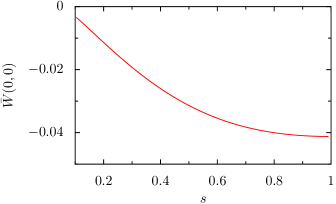
Figure 5: (color online). Minimal value of the Wigner function, $\bar{W}(0,0)$, as a function of squeezing parameter $s=\exp(-2r)$, which is varied by changing the quantity $qlE_{0}$. The narrow-filter approximation was made for the spectral slit. Fixed parameters: pulse parameters $w=1.2w_{P}$, $\tau_{P}=\tau=150\,{\rm fs}$, transmission of sampling beam splitter $\mathrm{T}=90\%$, efficiency of homodyne detection $\eta_{\rm hom}=0.93$.

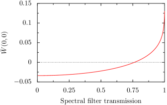
Figure 6: (color online). Minimal value of the Wigner function, $\bar{W}(0,0)$, as a function of the spectral slit transmission for the homodyne mode. Calculated for $s=0.56$, using a complete evaluation of integrals  (49), i.e. without the narrow-filter approximation. The narrow-filter approximation is well satisfied for low transmissions.

In Ref. Ourjoumtsev2006a , the best experimental results (highest modal purities) were obtained for $s=0.56$. For this value of $s$, which can be selected by choosing the right value for the quantity $qlE_{0}$, we obtain $g=0.50$ and $\bar{W}(0,0)=-0.034$; the latter value is close to what was observed in Ourjoumtsev2006a , without correction for the detection efficiency. At this stage, it can be interesting to compare this result, obtained using the narrow-filter approximation, with a more accurate calculation based on a complete evaluation of integrals  (49). Figure 6 presents the numerical results obtained for $\bar{W}(0,0)$ at $s=0.56$ as a function of the spectral slit transmission for the homodyne mode. (This transmission can be increased by making the spectral slit width $\Omega$ larger.) A minimal value is clearly reached for low transmissions, justifying a posteriori the use of narrow spectral slits in the experiment of Ref. Ourjoumtsev2006a . Since for low transmissions, $\bar{W}(0,0)$ does not differ much from its minimal value, the narrow-filter approximation that we made in Sec. III.3 gives accurate results.

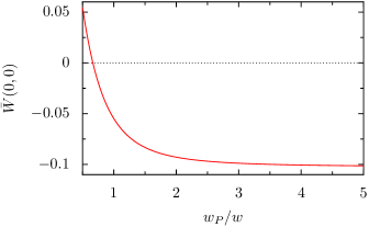
Figure 7: (color online). Minimal value of the Wigner function, i.e. $\bar{W}(0,0)$, as a function of $w_{P}/w$, where $w_{P}$ is the waist of the pump field and $w$ is the waist of the homodyne field. $qlE_{0}$ is fixed such that squeezing parameter $s=0.56$. Other parameter values as in Fig. 5.

Figure 7 predicts the behavior of $\bar{W}(0,0)$ when varying the size of the pump beam. Experimental values for the widths were related by $\omega=1.2\omega_{P}$ Ourjoumtsev2006a . Fig. 7 clearly shows that one can await a high increase of the negativity from a larger pump beam. This result was intuitive, as there is less gain-induced distortions in that case, but is here quantified. This can motivate the use of amplified pulses Dantan , in order to have a spatially broader pump beam (i.e. with larger $w_{P}$), but with the same intensity.

Comparison with empirical model.— Measured negative Wigner functions were interpreted in Ourjoumtsev2006a using the empirical model as introduced in Sec. III.2, where the photon is subtracted in the ‘good’ mode $\hat{a}_{h,{\rm out}}$ with probability $\xi$, and where the state is left in the squeezed vacuum with probability $(1-\xi)$. As explained before, the main difference between the empirical and our models is that the conditioned state in the former corresponds to the single-photon initial state $\hat{a}^{\dagger}_{\theta_{0}}$ with $\tan\theta_{0}=\beta/\alpha$, while it corresponds to $\hat{a}^{\dagger}_{\bar{\theta}}$ in the latter, with $\tan\bar{\theta}=\bar{\delta}/\bar{\gamma}$. These angles $\theta_{0}$ and $\bar{\theta}$ are mixing angles that fix the probability amplitudes of detection of a photon of mode 0 and of mode 1. Figure 8 shows $\theta_{0}$ and $\bar{\theta}$ as a function of the squeezing parameter $s$. Clearly, $\theta_{0}$ and $\bar{\theta}$ do not differ too much, and by less than $10\%$ for $s=0.56$.

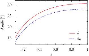
Figure 8: (color online). Mixing angles $\bar{\theta}$ (solid line) and $\theta_{0}$ (dashed line) of modes 0 and 1, as a function of squeezing parameter $s$, which is varied by changing $qlE_{0}$. Other parameter values as in Fig. 5.

Another important difference between our model and the empirical model is that modal purities $\xi_{j}$ in our model are fixed by the relation (20), whereas the parameter $\xi$ in the empirical model is a free parameter. This freedom can be used to fit the data, i.e. to have $A_{\rm emp}=\bar{A}$ or $B_{\rm emp}=\bar{B}$. It is however not a priori possible to fit both parameters $\bar{A}$ and $\bar{B}$ (52a,52b) from (39) using only the fitting parameter $\xi$. In neither model should the variances $V_{x}$ and $V_{p}$ be considered as free fitting parameters of the photon-subtraction experiment, at least their values should agree with the values for $V_{x,p}$ obtained by homodyne measurements of the squeezed vacuum.

In our model the mixing angles $\theta_{j}$ and their average $\bar{\theta}$ take into account the filtering of the signal that is used for conditioning. In the empirical model, the corresponding angle $\theta_{0}$ is independent of the filtering. Thus it is to be expected that this inaccuracy of the empirical model will lead to optimally fitted modal purities $\xi_{\rm opt}$ in the empirical model that are systematically lower than the average modal purity $\bar{\xi}$ in our model. This is indeed what we find for the curves in Figure 9: the best fit in the present example is obtained for $\xi_{\rm opt}=0.87$, a value that is indeed smaller but still close to $\overline{\xi}\approx 0.91$. The high quality of this fit (with an error less than $1.2\%$) is directly linked to the fact that in the present case $\theta_{0}\approx\overline{\theta}$.

There is a possibility to improve this result if $g$ is considered as a fitting parameter as well. We obtained an error of less than $0.4\%$ between the Wigner functions for $\xi_{\rm opt}=0.89$ and $g_{\rm opt}=0.53$, i.e. for a value of $g$ that differs by $6\%$ from the value given by the multimode model. In other words, if $g$ has a great influence on $A_{\rm emp}$ and $B_{\rm emp}$ in (39), it has a very low impact on $V_{x}$, $V_{p}$; the change from $g=0.50$ to $g_{\rm opt}=0.53$ modifies the values of $V_{x}$, $V_{p}$ by only a few $10^{-3}$, and for this reason it is very difficult to accurately measure $g$ from squeezed vacuum Wenger . These considerations explain why the empirical model can fit experimental data so successfully; even when $\theta_{0}$ is not equal to $\bar{\theta}$, the parameter $g$ gives a supplementary freedom for fitting.

Figure 9: (color online). Sections along $(x,0)$ and $(0,p)$ of the Wigner function $\bar{W}(x,p)$ (solid line), and corresponding best fits using the empirical model (dashed line) with $\xi_{\rm opt}=0.87$. Parameter values as in Fig. 5. Results of our model and the empirical fits almost overlap.

IV Discussion and conclusions

We have introduced a straightforward and physically intuitive procedure that we call ‘mode reduction’ to simplify the multimode description of squeezed light to the bare essentials. For photon-subtraction experiments, this means that the homodyne signal is reduced to an effective two-mode description and the detector signal requires one extra orthogonal effective mode. We derived the Wigner function of the homodyne signal conditional upon the detection of a single photon, and we also showed how to average over possible measurement outcomes.

The general mode-reduction formalism was then applied to a detailed model describing photon subtraction of gaussian spatiotemporal pulses of squeezed light. This model features many experimental parameters such as beam waists and duration of the pulses that can be independently measured. Indeed, our model does not have free fitting parameters. This allows one to study in detail what are the crucial experimental parameters to produce optimally negative Wigner functions with pulses of squeezed light.

We compared our new model to the empirical model that was used before to analyze photon-subtraction experiments in Ourjoumtsev2006a . In fact, the formulae for the output Wigner functions look similar. One crucial difference is that the empirical model does have a free parameter, namely the quantity called the modal purity. In our model modal purities also occur, be it with a slightly different meaning, but they are fixed quantities. A good agreement between our model and experiments therefore gives more understanding than an accurate fit with the empirical model.

We found that in the range of parameters of the measurements in Ourjoumtsev2006a , both our model and the empirical model are accurate. We reasoned that modal purities in our model would be systematically higher, and in our numerical example we found this to be the case. The accuracy of the empirical model strongly depends on the availability of the free parameter. It was nevertheless a surprise in the theoretical analysis that the mixing angles $\theta_{0}$ and $\bar{\theta}$, describing the relative probability of measuring a photon in either one of two effective modes, differ at most $20\%$ in a whole range of squeezing parameters.

Our mode-reduction procedure is closely related to the analysis of photon-subtraction experiments of Refs. Molmer ; Nielsen2007a ; Nielsen2007b . One could express our mode-reduction parameters in terms of elements of the covariance matrix of Refs. Molmer ; Nielsen2007a ; Nielsen2007b . Our output Wigner function in Eq. (27) then reduces to the one in Ref. Nielsen2007b , but only in the special case that all our mode reduction parameters are real-valued so that $D_{j}$ in Eq. (28d) vanishes. This we assumed for simplicity in Sec. III.3. Our mode-reduction procedure is carried out in the Heisenberg picture. We think that our approach has some advantages. In our approach it becomes quite intuitive in what sense it goes beyond the empirical model of Ref. Ourjoumtsev2006a . In our concrete multimode analysis, we include effects not considered in Ref. Nielsen2007b , such as the transverse beam profile, for which we found that wider pump beams lead to more negative Wigner functions.

In conclusion, we presented a very concise model that can account for the multimode nature of projective photon-counting measurements. It gives an intuitive picture of photon-subtraction experiments, close to the empirical model previously published. This multimode model therefore gives consistent results, in agreement with previously published experiments where pulses of light with negative Wigner functions were produced conditionally. Our model can be used to predict the changes in the output upon variation of experimentally relevant parameters, and to optimize the setup design.

Appendix A Wigner function

In order to derive Eq. (27) from Eq. (II.4), one has first to invert Eqs. (7,22), leading to

$$\hat{a}_{0} = \eta(\hat{a}_{h,{\rm out}}-\frac{\beta\hat{a}^{\dagger}_{1,{\rm out}}}{\sqrt{1+\beta^{2}}})-\alpha(\hat{a}^{\dagger}_{h,{\rm out}}-\frac{\beta\hat{a}_{1,{\rm out}}}{\sqrt{1+\beta^{2}}})$$ (62)

$$\hat{a}_{1} = \sqrt{1+\beta^{2}}\hat{a}_{1,{\rm out}}-\beta\hat{a}^{\dagger}_{h,{\rm out}}.$$ (63)

One should then replace in Eq.(II.4) $x_{0,1},p_{0,1}$ by $x_{h,{\rm out}},p_{h,{\rm out}},x_{1,{\rm out}}$, and $p_{1,{\rm out}}$, and integrate over $x_{1,{\rm out}}$, $p_{1,{\rm out}}$. It is however convenient to make a change of variables so that the integral is over $x_{1}$, $p_{1}$ instead of $x_{1,{\rm out}}$, $p_{1,{\rm out}}$. In this case the only transforms needed for this calculation is

$$x_{0} = \frac{\eta-\alpha}{1+\beta^{2}}(x_{h,{\rm out}}-\beta x_{1})$$ (64a)

$$p_{0} = \frac{\eta+\alpha}{1+\beta^{2}}(p_{h,{\rm out}}+\beta p_{1}),$$ (64b)

as well as the transformation of the integral

$$\int\mbox{d}x_{1,{\rm out}}\mbox{d}p_{1,{\rm out}}=\frac{1}{1+\beta^{2}}\int\mbox{d}x_{1}\mbox{d}p_{1}.$$ (65)

One should then note that the Wigner function (II.4) is the product of a polynomial in $x$, $p$, and of a gaussian term $\exp{(-R^{2})}$, with

$$R^{2}=x_{0}^{2}+p_{0}^{2}+x_{1}^{2}+p_{1}^{2}=x_{\theta}^{2}+p_{\theta}^{2}+x_{\theta+\pi/2}^{2}+p_{\theta+\pi/2}^{2}.$$ (66)

With Eq. (64), the exponent can be rewritten as

$$R^{2} = \frac{V_{x}}{(\eta+\alpha)^{2}}\left(x_{1}-\frac{\beta x_{h,{\rm out}}}{V_{x}}\right)^{2}+\frac{x_{h,{\rm out}}^{2}}{V_{x}}$$

$$+ \frac{V_{p}}{(\eta-\alpha)^{2}}\left(p_{1}-\frac{\beta p_{h,{\rm out}}}{V_{p}}\right)^{2}+\frac{p_{h,{\rm out}}^{2}}{V_{p}}.$$

The integral (65) with Eq. (II.4) as its integrand can then be found by replacing in the integrand the squares $x_{1}^{2}$ and $p_{1}^{2}$ by

$$x_{1}^{2}\rightarrow\frac{\beta^{2}x_{h,{\rm out}}^{2}}{V_{x}^{2}}+\frac{(\eta+\alpha)^{2}}{2V_{x}}$$ (67a)

$$p_{1}^{2}\rightarrow\frac{\beta^{2}p_{h,{\rm out}}^{2}}{V_{p}^{2}}+\frac{(\eta-\alpha)^{2}}{2V_{p}},$$ (67b)

and by replacing the first-order terms according to

$$x_{1}\rightarrow\frac{\beta x_{h,{\rm out}}}{V_{x}}$$ (68a)

$$p_{1}\rightarrow\frac{\beta p_{h,{\rm out}}}{V_{p}}.$$ (68b)

Appendix B Slowly Varying Envelope Approximation

The goal of this appendix is the derivation of the local Bogoliubov transformation (41). We assume that inside the DOPA the pump pulse with an angular frequency $2\omega_{0}$ travels at a speed $v_{g,2\omega_{0}}$, with negligible absorption. This field can therefore be written as

$$\mathrm{i}\,E_{P}(x,y,t-\frac{z}{v_{g,2\omega_{0}}}-\delta t)\exp(2i\omega_{0}t-i\vec{k}_{2\omega_{0}}\cdot\vec{r}),$$ (69)

where $\delta t$ is an arbitrary time delay and where ‘$\mathrm{i}$’ is a purely conventional phase factor. Let us write the probe beam as

$$E(\vec{r},t)=A(\vec{r},t)\exp(i\omega_{0}t-i\vec{k_{\omega_{0}}}\cdot\vec{r}),$$ (70)

where the phase-matching condition $\vec{k}_{2\omega_{0}}=2\vec{k}_{\omega_{0}}$ is assumed to be satisfied. By using the SVEA in Maxwell’s equations, neglecting diffraction terms and considering the first-order dispersion, we obtain

$$\frac{\partial A}{\partial z}+\frac{1}{v_{g,\omega_{0}}}\frac{\partial A}{\partial t}=qE_{P}(x,y,t-\frac{z}{v_{g,2\omega_{0}}}-\delta t)A^{*},$$ (71)

where $A=A(\vec{r},t)$. The substitution of $t-z/v_{g,\omega_{0}}$ by $t$ then leads to

$$\frac{\partial A}{\partial z}(\vec{r},t)=qE_{P}(x,y,t-Dz-\delta t)A^{*}(\vec{r},t),$$ (72)

where $D=v^{-1}_{g,2\omega_{0}}-v^{-1}_{g,\omega_{0}}$ is the GVM. With the assumption that $E_{P}$ is real-valued, the solution to Eq. (72) becomes

$$A_{\rm out}=\cosh[\,qlF_{P}\,]\,A_{\rm in}+\sinh[\,qlF_{P}\,]\,A^{*}_{\rm in},$$ (73)

where the $(x,y,t)$-dependence was suppressed. The effective pump field $F_{P}$ is given by

$$F_{P}=\frac{1}{l}\int_{0}^{l}dzE_{P}=\frac{1}{\tau_{g}}\int_{\delta t}^{\tau_{g}+\delta t}d\tau E_{P}(x,y,t-\tau),$$ (74)

with $\tau_{g}=Dl$ the time separation induced by the GVM after crossing the crystal. Eq. (74) shows that the effective pump field $F_{P}$ is a convolution of the pump field $E_{P}$ with a rectangular unit gate of duration $\tau_{g}$, which for $\delta t=-\tau_{g}/2$ is centered around the origin. As the quantized version of Eq. (73), we then find Eq. (41) of the main text. The pump field $E_{P}$ of the main text is to be understood as the effective pump field $F_{P}$ derived here. Evidently, $F_{P}\rightarrow E_{P}$ in the limit $\tau_{g}\rightarrow 0$ (no GVM).

References

- (1) J. Eisert, S. Scheel, and M.B. Plenio, Phys. Rev. Lett. 89, 137903 (2002).
- (2) G. Giedke and J.I. Cirac, Phys. Rev. A 66, 032316 (2002).
- (3) D.E. Browne, J. Eisert, S. Scheel, and M.B. Plenio, Phys. Rev. A 67, 062320 (2003).
- (4) M.S. Kim, E. Park, P.L. Knight, and H. Jeong, Phys. Rev. A 71, 043805 (2005).
- (5) A. Biswas and G.S. Agarwal, Phys. Rev. A 75, 032104 (2007).
-
(6)
M. Dakna, T. Anhut, T. Opatrný, L. Knöll, and
D.-G. Welsch, Phys. Rev. A 55, 3184 (1997). - (7) T. Opatrný, G. Kurizki, and D.-G. Welsch, Phys. Rev. A 61, 032302 (2000).
- (8) A.I. Lvovsky, H. Hansen, T. Aichele, O. Benson, J. Mlynek, and S. Schiller, Phys. Rev. Lett. 87, 050402 (2001).
- (9) J. Wenger, R. Tualle-Brouri and P. Grangier, Phys. Rev. Lett. 92, 153601 (2004).
- (10) A. Ourjoumtsev, R. Tualle-Brouri, J. Laurat, and Ph. Grangier, Science 312, 83 (2006), and Supporting Online Material.
- (11) A. Ourjoumtsev, R. Tualle-Brouri, and Ph. Grangier, Phys. Rev. Lett. 96, 213601 (2006).
- (12) K. Wakui, H. Takahashi, A. Furusawa and M. Sasaki, e-print quant-ph/0609153v1.
- (13) J.S. Neergaard-Nielsen, B. Nielsen, C. Hettich, K. Mølmer, and E.S. Polzik, Phys. Rev. Lett. 97, 083604 (2006).
- (14) A. Ourjoumtsev, H. Jeong, R. Tualle-Brouri, P. Grangier, Nature 448, 784 (2007).
- (15) V. Parigi, A. Zavatta, M. Kim, and M. Bellini, Science 317, 1890 (2007).
- (16) M.S. Kim, J. Phys. B: At. Mol. Opt. Phys. 41, 133001 (2008).
- (17) M. Avenhaus, H. B. Coldenstrodt-Ronge, K. Laiho, W. Mauerer, I. A. Walmsley and C. Silberhorn, Phys. Rev. Lett. 101, 053601 (2008).
- (18) M. Sasaki and S. Suzuki, Phys. Rev. A 73, 043807 (2006).
- (19) K. Mølmer, e-print quant-ph/0602202v1.
- (20) A.E.B. Nielsen and K. Mølmer, Phys. Rev. A 75, 023806 (2007).
- (21) A.E.B. Nielsen and K. Mølmer, Phys. Rev. A 76, 033832 (2007).
- (22) F. Grosshans and Ph. Grangier, Phys. Rev. Lett. 88, 057902 (2002).
- (23) T. Aichele, A.I. Lvovsky and S. Schiller, Eur. Phys. J. D 18, 237 (2002).
- (24) A. La Porta and R. E. Slusher, Phys. Rev. A 44, 2013 (1991).
- (25) C.W. Gardiner and P. Zoller, Quantum Noise (Springer, Berlin, 2000).
- (26) J. Wenger, J. Fiurášek, R. Tualle-Brouri, N.J. Cerf, and P. Grangier, Phys. Rev. A 70, 053812 (2004).
- (27) U. Leonhardt, Measuring the Quantum state of Light (Cambridge University Press, 1997).
- (28) A. Dantan, J. Laurat, A. Ourjoumtsev, R. Tualle-Brouri, and P. Grangier, Optics Express 15, 8864 (2007).