Improving stellar parameter and abundance determinations of early B-type stars

Abstract

In the past years we have made great efforts to reduce the statistical and systematic uncertainties in stellar parameter and chemical abundance determinations of early B-type stars. Both the construction of robust model atoms for non-LTE line-formation calculations and a novel self-consistent spectral analysis methodology were decisive to achieve results of unprecedented precision. They were extensively tested and applied to high-quality spectra of stars from OB associations and the field in the solar neighbourhood, covering a broad parameter range. Initially, most lines of hydrogen, helium and carbon in the optical/near-IR spectral range were reproduced simultaneously in a consistent way for the first time, improving drastically on the accuracy of results in published work. By taking additional ionization equilibria of oxygen, neon, silicon and iron into account, uncertainties as low as $\sim$1% in effective temperature, $\sim$10% in surface gravity and $\sim$20% in elemental abundances are achieved – compared to $\sim$5-10%, $\sim$25% and a factor $\sim$2-3 using standard methods.

Several sources of systematic errors have been identified when comparing our methods for early B-type stars with standard techniques used in the nineties and also recently (e.g. VLT-FLAMES survey of massive stars). Improvements in automatic analyses are strongly recommended for meaningful comparisons of spectroscopic stellar parameters and chemical abundances (’observational constrains’) with predictions of stellar and galactochemical evolution models.

1. Introduction

Normal unevolved early OB-type stars of $\sim$8-20 M_⊙ are the objects with the simplest photospheric physics among the massive stars. They are unaffected by e.g. strong stellar winds like the hotter and more luminous stars or by convection and chromospheres like the cool supergiants. However, their spectral analysis turned out to provide inconclusive results in the past decades, i.e. too large uncertainties in basic stellar parameters and an overall enormous range in derived elemental abundances, posing a challenge to predictions of stellar and Galactochemical evolution models (see review by Przybilla 2008).

In order to improve the quantitative analysis of these stars we have exhaustively updated the spectral modelling by constructructing robust model atoms for non-LTE line-formation calculations. In parallel, we have implemented a powerful self-consistent analysis technique, which brings numerous spectroscopic parameter and abundance indicators into agreement simultaneously.

Our efforts have provided highly-promising results so far, i.e. a drastic reduction of statistical and systematic uncertainties in stellar parameters and chemical abundances (Nieva & Przybilla 2007, 2008; NP07/08). As a first application, stars from OB associations and the field in the solar neighbourhood covering a broad parameter range were analysed. The sample turned out to be chemically homogeneous on the $\sim$10% level (Przybilla, Nieva & Butler 2008, PNB08), corroborating earlier findings from analyses of the ISM gas-phase. The data are also consistent with published Orion nebula abundances. The results have an immediate impact on several fields of contemporary astrophysics like stellar (see Przybilla, Firnstein & Nieva, these proceedings) and Galactic chemical evolution models and the dust-phase composition of the local ISM. They provide an independent view on the discussion of photospheric solar abundances and helioseismic constraints on the solar interior model, and they define the initial chemical composition for models of star and planet formation in the solar neighbourhood. In addition, a few B-type hyper-velocity stars were analysed using this technique, providing valuable constraints on their nature and their ejection mechanisms (Przybilla et al. 2008a,b).

Despite this kind of star has relatively simple photospheres compared to other objects, the spectral analysis is still sensitive to many potential systematic effects which are usually underestimated. We discuss the most common sources of systematic error that have to be avoided when high precision/accuracy in spectral analyses is desired. Observational constraints as obtained from automatic spectral analyses of large star samples like the VLT-FLAMES survey of massive stars may benefit significantly from a proper elimination of these systematics.

2. Model calculations and new spectral analysis methodology

A hybrid approach is used for the non-LTE line-formation computations. These are based on line-blanketed plane-parallel, homogeneous and hydrostatic LTE model atmospheres calculated with Atlas9. Non-LTE synthetic spectra are computed with recent versions of Detail and Surface. These codes solve the coupled radiative transfer and statistical equilibrium equations and compute synthetic spectra using refined line-broadening data, respectively. The hybrid non-LTE approach is consistent with full non-LTE calculations (NP07) but faster and it also allows comprehensive model atoms based on critically selected atomic data to be employed in the non-LTE line-formation computations.

The new spectral analysis was originally based on a self-consistent and simultaneous reproduction of almost all hydrogen, helium and carbon lines in the optical/near-IR spectra, matching multiple ionization equilibria (He i/ii, C ii/iii/iv), see Nieva & Przybilla (2006), NP07 and NP08 for details. The method was further extended by consideration of additional ionization equilibria (O i/ii, Ne i/ii, Si ii/iii/iv, Fe ii/iii, PNB08). This allows unprecedently accurate stellar parameters and elemental abundances to be derived, with uncertainties as low as $\sim$1% in effective temperature $T_{\rm eff}$, $\sim$10% in surface gravity $g$ and $\sim$20% in elemental abundances. Significant improvements on results from previous studies are thus achieved, which typically give uncertainties of $\sim$5-10%, $\sim$25% and a factor $\sim$2-3 for these quantities. Moreover, the successful implementation of the new method required an identification of sources of systematic uncertainties in standard spectral analyses and allowed in most cases for their quantification, which we discuss in the following.

3. Reducing systematic uncertainties

Every step in a quantitative spectral analysis is susceptible to systematic uncertainties. Here we briefly list the most common sources of systematics that affect the final error in stellar parameters and elemental abundances of normal unevolved early B-type stars. When possible, recipies are given how to prevent them. Additional systematics may arise from further complications like magnetic fields, but this is beyond the present scope.
Single or double? Not only spectroscopic but also close visual binaries are expected to be observed in dense fields. Standard analyses for single stars applied to a spectrum contaminated with light of a second star can give erroneous results throughout. Inspection of H or He lines can help to identify asymmetries due to a companion before carring out an automatised quantitative analysis.
Quality of spectra. Continuum normalization, local continuum definition and low S/N are important sources of systematics. E.g., spectra of S/N$\sim$50 challenge the definition of the local continuum of spectral lines. The abundance determination in stars rotating at intermediate velocities ($v\sin i\sim 50\,\mathrm{km\,s^{-1}}$) is limited to 0.2-0.3 dex in accuracy at this S/N. Fast-rotating stars ($v\sin i\geq 150\,\mathrm{km\,s^{-1}}$) or low-resolution spectra impose even more complications because metal line blends lower the real continuum, hence the abundances can be systematically underestimated and the accuracy is limited to 0.3-0.4 dex (see Korn et al. 2005).
Model atmospheres and line formation. Atmospheric structures computed with full non-LTE or hybrid non-LTE methods are equivalent for unevolved B stars (NP07), when the abundances used for opacity calculations are the same – note that ‘solar’ abundances have changed over time. Line-blanketing effects on the atmosphere impact the line-formation calculations, introducing dependencies on metallicity and microturbulence. In a similar way, line blocking affects the strength of synthetic lines by modifying radiative rates. Both effects need to be accounted for in a consistent way.
Model atoms. Most model atoms for non-LTE calculations are based on input atomic data (ab-initio and approximation data) as available in the early nineties. It is worthwhile to check for improvements on the modelling whenever new data becomes available. E.g., for C different model atoms yield discrepancies in abundances up to 0.8 dex for some lines while no discrepancies are found for others, see Sect. 3.1. and NP08. Other elements also show a similar behaviour.

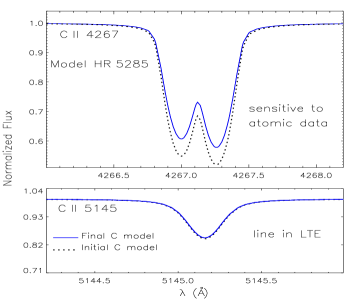
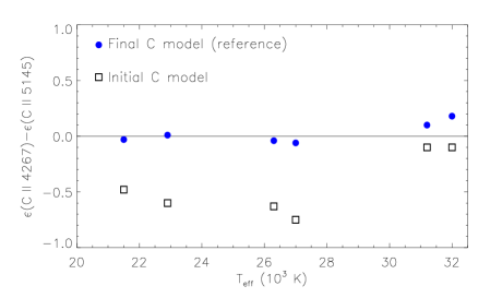
Figure 1.: Left: sensitivity of two C ii lines to use of photoionization cross-sections from different ab-initio calculations in a model spectrum for a B2 V star. Right: differences in C abundance as derived from the two lines in 6 stars as a function of $T_{\rm eff}$. From NP08, see text for details.

Effective temperatures. $T_{\mathrm{eff}}$ estimated from photometry can differ from those determined with the self-consistent spectroscopic method by more than 10% (NP08). Spectroscopic determinations via ionization equilibria are a powerful technique only when the model atoms are reliable. In addition, one ionization equilibrium alone does not provide accurate constraints because of dependencies on other variables like microturbulence (see below, Fig. 2 and consequences for C abundances in Table 1). Therefore, only the simultaneous use of multiple ionization equilibria provides a reliable and parameter-free $T_{\mathrm{eff}}$ determination.
Surface gravity. The common use of only one Balmer line as $\log\,g$ indicator does not allow for consistency checks. Instead, most Balmer lines and metal ionization equilibria should be considered for an accurate determination. Moreover, neglecting non-LTE effects also leads to systematic errors: increasing with $T_{\mathrm{eff}}$ up to $\sim$0.2 dex in $\log\,g$ around 35 000 K, see NP07/08 and Sect. 3.1. Ionization equilibria can also be a powerful tool for the $\log g$ determination.
Microturbulence. This quantity is generally derived from selected lines of one oxygen or one silicon ion. However, the microturbulent velocity $\xi$ should adopt the same value for all metals. In particular, cross-checks including different species are mandatory when only a few lines are measurable (like in fast rotators) in order to avoid large uncertainties. Microturbulent velocities often come close to or exceed the sound speed in many previous studies. In contrast, physically more reasonable lower values are found in our work, increasing from $\sim$2-4 ${\rm km\,s}^{-1}$ in dwarfs to $\sim$5-8 ${\rm km\,s}^{-1}$ in giants. Consequences of overestimated $\xi$ for the $T_{\mathrm{eff}}$ and abundance determination are discussed in Sect. 3.1.
Spectral line selection. Abundances may depend on the selection of lines used in the analysis when the model atoms are not comprehensive: some multiplets may indicate systematically different abundances than others. Moreover, some lines are observable only in cooler or in hotter stars. Which lines should one choose for the analysis? All possible observed lines for each star should be taken into account in the optimum case (see NP08 and PNB08).
Non-LTE corrections. Non-LTE effects cannot be easily predicted. They affect different lines of the same star in different ways. Non-LTE line strengthening or weakening can occur, and non-LTE effects are not restricted to stronger lines alone. For different plasma conditions the non-LTE effects change. Hence, adding or subtracting fixed ‘non-LTE abundance corrections’ to LTE results may increase the systematics.
Macroturbulence. Macroturbulence is not considered in many studies. This is important for proper $v\sin i$ determinations in apparently slow-rotating objects.

3.1. Systematics from atomic data and atmospheric parameters

Here we provide a few quantitative examples of systematic effects on abundance analyses to be expected due to use of different input atomic data for non-LTE calculations and due to atmospheric parameter variations.

Fig. 1 shows discrepant results for C ii lines predicted by two different non-LTE model atoms. On the left panel the sensitivity of two lines to different ab-initio photoionization cross-sections is shown. Inaccurate atomic data will indicate largely underestimated abundances for the stronger line. This is quantified for stars within a broad parameter range (right panel). The discrepancies in abundances depend on the reliability of the model atom and on the plasma conditions of the star and amount up to 0.8 dex. In parallel, collisional excitation and ionization cross-sections and $\log\,gf$ values need to be reliable (NP08).

Figure 2.: Effective temperature determination via Si ionization equilibrium for the LMC star NGC2004-D15. The Si iii lines are strong, hence the derived Si iii abundance depends on the microturbulence $\xi$. Different $T_{\mathrm{eff}}$ is derived from Si ii/iii and Si iii/iv for ill-chosen $\xi$, e.g. an overestimation of $\xi$ by 7 km s^-1 gives $\Delta T_{\mathrm{eff}}$ $\approx$ 2000 K. The Si ii/iii/iv ionization equilibrium is established only for the correct $\xi$ (from Nieva 2007).

Table 1.: Systematic errors in C abundances of individual lines caused by atmospheric parameter variations and the assumption of LTE for the line-formation calculations in the B1 III star HR 3055 ($T_{\mathrm{eff}}=31\,200\pm 300$ K; $\log g=3.95\pm 0.05$; $\xi=8\pm 2\,\rm{km\,s^{-1}}$, see NP08, PNB08)

$$\footnotesize{\begin{array}[]{lcccccccc}\cr\hline\cr\mathrm{Ion}&\lambda&W_{\lambda}&\mathrm{\varepsilon(C)_{\mathrm{NLTE}}}&\Delta T_{\mathrm{eff}}&\Delta\log\,g&\Delta\,\xi&\mathrm{LTE}\\ &\mathrm{(\AA)}&\mathrm{(m{\AA})}&&-2000\,\mathrm{K}&+0.2\,\mathrm{dex}&+5\,\mathrm{km\,s}^{-1}&\\ \hline\cr\\[-5.69054pt] \rm C$\,{\sc ii}$&4267.2&113&8.46&-0.33&-0.11&-0.16&-0.40\\[-1.42262pt] &5133.3&19&8.34&-0.30&-0.10&~{}~{}0.00&~{}~{}0.00\\[-1.42262pt] &5143.4&10&8.44&-0.40&-0.05&~{}~{}0.00&~{}~{}0.00\\[-1.42262pt] &5145.2&19&8.36&-0.32&-0.09&-0.02&~{}~{}0.00\\[-1.42262pt] &5151.1&11&8.34&-0.30&-0.08&~{}~{}0.00&~{}~{}0.00\\[-1.42262pt] &5662.5&~{}4&8.37&-0.33&-0.13&~{}~{}0.00&~{}~{}0.00\\[-1.42262pt] &6578.0&66&8.24&-0.40&-0.15&-0.10&~{}~{}0.00\\[-1.42262pt] &6582.9&37&8.29&-0.30&+0.02&+0.05&+0.05\\[2.84526pt] \rm C$\,{\sc iii}$&4056.1&45&8.28&+0.21&+0.06&-0.04&+0.08\\[-1.42262pt] &4162.9&58&8.29&+0.28&+0.09&-0.03&+0.25\\[-1.42262pt] &4186.9&92&8.34&+0.35&+0.15&-0.08&+0.07\\[-1.42262pt] &4663.5&18&8.27&+0.22&+0.07&-0.03&+0.22\\[-1.42262pt] &4665.9&50&8.24&+0.26&+0.08&-0.08&+0.35\\[-1.42262pt] &5272.5&14&8.28&+0.16&+0.01&~{}~{}0.00&~{}~{}0.00\\[2.84526pt] \rm C$\,{\sc iv}$&5801.3&53&8.45&+1.06&+0.46&-0.03&+0.39\\[-1.42262pt] &5811.9&34&8.45&+1.06&+0.46&-0.03&+0.39\\[-1.42262pt] \hline\cr\end{array}}$$

Fig. 2 shows the dependency of $T_{\mathrm{eff}}$ to the adopted value of microturbulence when only one ionization equilibrium of Si is adopted, i.e. Si ii/iii or Si iii/iv. This will also affect the derivation of $\log\,g$ from the Balmer lines. This problem can be solved via use of multiple ionization equilibria, e.g. Si ii/iii/iv and when possible also considering other elements (as explained above). The goal should be deriving the same value of $T_{\mathrm{eff}}$, $\log\,g$ and $\xi$ from all H, He and all metals.

Systematic errors in C abundances from individual lines in a B1 III star due to variations in $T_{\mathrm{eff}}$, $\log\,g$ and $\xi$ have been quantified in Table 1. The offsets in parameters are averaged discrepancies for studies using standard analysis techniques. Incorrect parameters prevent consistent C ii/iii/iv ionization equilibria to be achieved, even when the model atom is highly reliable in the defined parameter range. Parameters derived from C ionization equilibrium (NP08) are confirmed by other metals (PNB08) when reliable model atoms are used.

4. Conclusions

In the past years we have made great efforts to reduce uncertainties in quantitative spectral analyses of early B-type stars. A self-consistent analysis, i.e. account of all spectroscopic indicators – Balmer and helium lines and multiple metal ionization equilibria – throughout the optical and near-IR, resulted in drastically reduced systematic effects in the atmospheric parameter and elemental abundance determination. A large number of potetial systematic errors was identified when comparing our new models and self-consistent method with standard techniques. One should keep in mind that statistics does by no mean reduce systematic errors. We conclude that careful improvements in automatic spectral analysis routines should be implemented before being applied to large samples of stellar spectra. This will prevent unnecessary systematic bias in stellar parameters and abundance determinations, inconclusive results and misinterpretations of the studies by theoreticians. Comparisons of ’observational constraints’ and theoretical predictions are only meaningful when the former are unbiased by systematic error.

Acknowledgments.

The authors thank D. J. Lennon and D. J. Hillier for fruitful discussions.

References

- (1) Korn, A. J., Nieva, M. F., Daflon, S., & Cunha, K. 2005, ApJ, 633, 899
- (2) Nieva, M. F., & Przybilla, N. 2006, ApJ, 639, L39 (NP06)
-
(3)
Nieva, M. F. 2007, Ph.D. Thesis Univ. Erlangen-Nuremberg and
Obs. Nacional/MCT,
Verkannten Verlag (Berlin) - (4) Nieva, M. F., & Przybilla, N. 2007, A&A, 467, 295 (NP07)
- (5) Nieva, M. F., & Przybilla, N. 2008, A&A, 481, 199 (NP08)
- (6) Przybilla, N. 2008, Rev. Mod. Astron., 20, 323
- (7) Przybilla, N., Nieva, M. F., & Butler, K. 2008, ApJ, 688, L103 (PNB08)
- (8) Przybilla, N., Nieva, M. F., Heber, U., et al. 2008a, A&A, 480, L37
- (9) Przybilla, N., Nieva, M. F., Heber, U., & Butler, K. 2008b, ApJ, 684, L103