Quantum theory of optical temporal phase and instantaneous frequency. II. Continuous time limit and state-variable approach to phase-locked loop design

Abstract

We consider the continuous-time version of our recently proposed quantum theory of optical temporal phase and instantaneous frequency [Tsang, Shapiro, and Lloyd, Phys. Rev. A 78, 053820 (2008)]. Using a state-variable approach to estimation, we design homodyne phase-locked loops that can measure the temporal phase with quantum-limited accuracy. We show that post-processing can further improve the estimation performance, if delay is allowed in the estimation. We also investigate the fundamental uncertainties in the simultaneous estimation of harmonic-oscillator position and momentum via continuous optical phase measurements from the classical estimation theory perspective. In the case of delayed estimation, we find that the inferred uncertainty product can drop below that allowed by the Heisenberg uncertainty relation. Although this result seems counter-intuitive, we argue that it does not violate any basic principle of quantum mechanics.

I Introduction

Optical phase measurements at the fundamental quantum limit of accuracy are an important goal in science and engineering and crucial for future metrology, sensing, and communication applications. While the single-mode case has been extensively studied, less attention has been given to the quantum measurements of a temporally varying phase. Theoretically, the temporal-phase positive operator-valued measure (POVM) describes the optimal quantum measurements tsang , but it is difficult to perform such measurements in practice. Adaptive homodyne detection wiseman ; armen is a much more feasible approach, and Berry and Wiseman have proposed the use of a homodyne phase-locked loop to estimate the phase when the mean phase is a classical Wiener random process berry ; pope . On the other hand, we have recently shown in Ref. tsang how homodyne phase-locked loops can be designed using classical estimation theory to perform quantum-limited temporal phase measurements when the mean phase is any stationary Gaussian random process.

The main purpose of this paper is to unify and generalize the two distinct approaches undertaken by Berry and Wiseman and ourselves, under the common framework of classical estimation theory. In Sec. II, we first extend our discrete-time theory proposed in Ref. tsang to the continuous time domain. In Sec. III.1, we generalize Berry and Wiseman’s results to a much wider class of random processes using the Kalman-Bucy filtering theory vantrees ; baggeroer . The Kalman-Bucy approach guarantees the real-time estimation efficiency provided that the phase-locked loop operates in the linear regime. Our approach also significantly simplifies the design of phase-locked loops, compared to the more computationally expensive Bayesian state estimation approach suggested by Pope et al. pope . In Sec. III.2, we show that the Wiener filtering technique used in our previous paper tsang is equivalent to Kalman-Bucy filtering at steady state. In Sec. IV, we point out that Berry and Wiseman’s results are not optimal if delay is permitted in the phase estimation process, and post-processing can further improve the phase estimation performance beyond that offered by Kalman-Bucy or Wiener filtering. We illustrate these concepts by considering the specific cases of the mean phase being an Ornstein-Uhlenbeck random process as well as the Wiener process studied by Berry and Wiseman. Apart from the theoretical importance of our results in the context of quantum estimation and control theory, they should also be of immediate interest to experimentalists and engineers who wish to achieve quantum-limited temporal phase measurements, as we expect our proposals to be realizable using current technology.

In Sec. V, we investigate the fundamental problem of simultaneous harmonic-oscillator position and momentum estimation at the quantum limit by continuous optical phase measurements. The problem can be cast directly in the framework of classical estimation theory for Gaussian states. The use of Kalman-Bucy filtering for real-time position and momentum estimation has been proposed by Belavkin and Staszewski belavkin and Doherty et al. doherty , who have shown that the quantum state of the harmonic oscillator conditioned upon the real-time measurement record is a pure Gaussian state. Here we show that the inferred position and momentum estimation errors according to classical estimation theory can be further reduced below the Heisenberg uncertainty product, if delay is allowed in the estimation. While counter-intuitive, we explain in Sec. V.3 why this result does not violate the basic principles of quantum mechanics.

II Phase in the continuous time domain

For completeness, we first review the continuous time limit of our discrete-time theory of temporal phase tsang , as previously described in Ref. tsang_qcmc . Consider the optical envelope annihilation and creation operators $\hat{A}(t)$ and $\hat{A}^{\dagger}(t)$, respectively, in the slowly varying envelope regime, with the time-domain commutation relation

$$\left[\hat{A}(t),\hat{A}^{\dagger}(t^{\prime})\right] =\delta(t-t^{\prime}).$$ (1)

Let $dn(t)$ be a continuous-time discrete-photon-number random process, a realization of which is depicted in Fig. 1, and $\tau_{j}$ be the times at which $dn(\tau_{j})$ is non-zero.

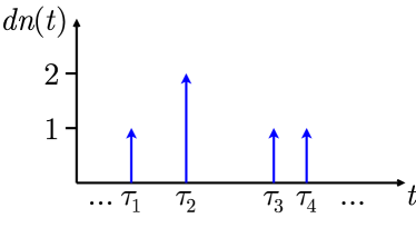
Figure 1: (Color online). A realization of the continuous-time discrete-photon-number random process.

A Fock state with a definite $dn(t)$ can be defined as

$$|dn(t)\rangle \equiv\left\{\prod_{j}\frac{1}{\sqrt{dn(\tau_{j})!}}\left[\hat{A}^{\dagger}(\tau_{j})\sqrt{dt}\right]^{dn(\tau_{j})}\right\}|0\rangle,$$ (2)

which is an eigenstate of the photon-number flux operator $\hat{A}^{\dagger}(t)\hat{A}(t)$,

$$\hat{A}^{\dagger}(t)\hat{A}(t)|dn(t)\rangle =I(t)|dn(t)\rangle,$$ (3)

$$I(t)\equiv\frac{dn(t)}{dt} =\sum_{j}dn(\tau_{j})\delta(t-\tau_{j}).$$ (4)

The Fock states form a complete orthogonal basis of the continuous-time Hilbert space,

$$\sum_{dn(t)}|dn(t)\rangle\langle dn(t)| =\hat{1},$$ (5)

where the sum is over all realizations of $dn(t)$. For a quantum state $\hat{\rho}$, the photon-number probability distribution is

$$P[dn(t)] =\operatorname{Tr}\left\{\hat{\rho}|dn(t)\rangle\langle dn(t)|\right\}, \sum_{dn(t)}P[dn(t)] =1.$$ (6)

For example, a coherent state is defined as

$$|\mathcal{A}(t)\rangle =\exp\left[-\frac{\bar{N}}{2}+\int_{-\infty}^{\infty}dt\mathcal{A}(t)\hat{A}^{\dagger}(t)\right]|0\rangle,$$

$$\bar{N} \equiv\int_{-\infty}^{\infty}dt|\mathcal{A}(t)|^{2},\quad\hat{A}(t)|\mathcal{A}(t)\rangle=\mathcal{A}(t)|\mathcal{A}(t)\rangle,$$ (7)

where $\mathcal{A}(t)$ is the mean field. The photon-number probability density is then

$$P[dn(t)] =\lim_{\delta t\to dt}e^{-\bar{N}}\prod_{j}\frac{\left[|\mathcal{A}(t_{j})|^{2}\delta t\right]^{dn(t_{j})}}{dn(t_{j})!},$$

$$t_{j} \equiv t_{0}+j\delta t,$$ (8)

which describes a Poisson process, as is well known hudson .

A temporal phase state can be defined as the functional Fourier transform of the Fock states,

$$|\phi(t)\rangle \equiv\sum_{dn(t)}\exp\left[i\sum_{j}dn(\tau_{j})\phi(\tau_{j})\right]|dn(t)\rangle$$

$$=\sum_{dn(t)}\exp\left[i\int_{-\infty}^{\infty}dtI(t)\phi(t)\right]|dn(t)\rangle.$$ (9)

In terms of the temporal phase states, a temporal-phase POVM can be defined as

$$\hat{\Pi}\left[\phi(t)\right] \equiv|\phi(t)\rangle\langle\phi(t)|,$$ (10)

which is the continuous limit of the one defined in Ref. tsang and can be normalized using a path integral with the paths restricted to a range of $2\pi$,

$$\int D\phi(t)\hat{\Pi}\left[\phi(t)\right] =\hat{1},\quad D\phi(t)\equiv\lim_{\delta t\to dt}\prod_{j}\frac{d\phi(t_{j})}{2\pi},$$

$$\phi_{0}(t) \leq\phi(t)<\phi_{0}(t)+2\pi.$$ (11)

The temporal-phase probability density is thus given by

$$p[\phi(t)] =\operatorname{Tr}\left\{\hat{\rho}\hat{\Pi}[\phi(t)]\right\}, \int D\phi(t)p[\phi(t)] =1.$$ (12)

It is difficult to analytically calculate $p[\phi(t)]$ for most quantum states of interest, so perturbative or numerical methods should be sought.

For the design of homodyne phase-locked loops, the Wigner distribution is of more interest. For a Gaussian state with uncorrelated quadratures, it can be written as

$$\quad W[\xi_{1}(t),\xi_{2}(t)]$$

$$\propto\exp\left[-\frac{1}{2}\sum_{j=1,2}\int dtd\tau\xi_{j}(t)K_{j}^{-1}(t,\tau)\xi_{j}(\tau)\right],$$ (13)

where $\xi_{j}(t)$ are quadrature processes,

$$\xi_{1}(t) \equiv A(t)e^{-i\theta(t)}+A^{*}(t)e^{i\theta(t)}$$

$$\quad-\left\langle A(t)e^{-i\theta(t)}+A^{*}(t)e^{i\theta(t)}\right\rangle,$$ (14)

$$\xi_{2}(t) \equiv-i\left[A(t)e^{-i\theta(t)}-A^{*}(t)e^{i\theta(t)}\right]$$

$$\quad-\left\langle-i\left[A(t)e^{-i\theta(t)}-A^{*}(t)e^{i\theta(t)}\right]\right\rangle,$$ (15)

$A(t)$ is the complex field variable in phase space, $\theta$ is an arbitrary phase, and $K_{j}^{-1}(t,\tau)$ is defined in terms of the covariance functions $K_{j}(t,\tau)$ as

$$\int duK_{j}(t,u)K_{j}^{-1}(u,\tau) =\delta(t-\tau),$$ (16)

$$K_{j}(t,\tau) \equiv\left\langle\xi_{j}(t)\xi_{j}(\tau)\right\rangle.$$ (17)

The covariance functions must satisfy the uncertainty relation

$$\int duK_{1}(t,u)K_{2}(u,\tau) \geq\delta(t-\tau),$$ (18)

which becomes an equality if and only if the state is pure. In particular, the covariance functions for a coherent state are

$$K_{1}(t,\tau) =K_{2}(t,\tau)=\delta(t-\tau).$$ (19)

III Phase-locked loop design

III.1 Kalman-Bucy filtering

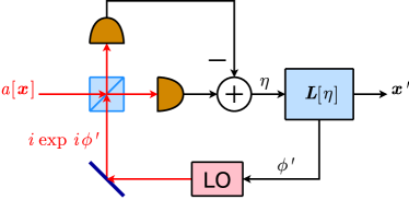
Figure 2: (Color online). A homodyne phase-locked loop. LO denotes local oscillator.

Consider the homodyne phase-locked loop illustrated in Fig. 2. The output of the homodyne detection can be written as

$$\eta(t) =\sin[\bar{\phi}(t)-\phi^{\prime}(t)]+z(t),$$ (20)

where $\bar{\phi}(t)$ is the mean phase of the optical field, which contains the message to be estimated, $\phi^{\prime}(t)$ is the local-oscillator phase, and $z(t)$ is the quantum noise. For a phase-squeezed state with squeezed quadrature $\xi_{2}(t)$ and anti-squeezed quadrature $\xi_{1}(t)$, $z(t)$ can be written as

$$z(t) \equiv\frac{1}{2|\mathcal{A}|}\Big{\{}\xi_{1}(t)\sin[\bar{\phi}(t)-\phi^{\prime}(t)]$$

$$\quad+\xi_{2}(t)\cos[\bar{\phi}(t)-\phi^{\prime}(t)]\Big{\}},$$ (21)

where $\mathcal{A}\equiv\langle\hat{A}\rangle=|\mathcal{A}|\exp(i\bar{\phi})$ is the mean field. For generality, we let the message be a vector of $n$ random processes,

$$\boldsymbol{x}(t) \equiv\left[\begin{array}[]{c}x_{1}(t)\\ x_{2}(t)\\ \vdots\\ x_{n}(t)\end{array}\right],$$ (26)

with the mean phase proportional to the first one,

$$\bar{\phi}(t) =\boldsymbol{C}(t)\boldsymbol{x}(t), \boldsymbol{C}(t) \equiv[\beta,0,\dots,0].$$ (27)

In the Kalman-Bucy formalism, $\boldsymbol{x}(t)$ is modeled as zero-mean random processes that satisfy a set of linear differential equations,

$$\frac{d\boldsymbol{x}(t)}{dt} =\boldsymbol{A}(t)\boldsymbol{x}(t)+\boldsymbol{B}(t)\boldsymbol{u}(t),$$ (28)

where $\boldsymbol{A}(t)$ and $\boldsymbol{B}(t)$ are $n\times n$ and $n\times m$ matrices, respectively, and $\boldsymbol{u}(t)$ is a vector of $m$ zero-mean white Gaussian inputs with autocorrelation

$$\left\langle\boldsymbol{u}(t)\otimes\boldsymbol{u}(\tau)\right\rangle =\boldsymbol{U}\delta(t-\tau).$$ (29)

We focus on coherent states, so that $z(t)$ can be modeled as an independent white Gaussian noise according to its Wigner distribution,

$$\left\langle z(t)z(\tau)\right\rangle =Z(t)\delta(t-\tau), Z(t) \equiv\frac{1}{4|\mathcal{A}|^{2}}=\frac{\hbar\omega_{0}}{4\mathcal{P}}.$$ (30)

where $\omega_{0}$ is the optical carrier frequency and $\mathcal{P}$ is the average optical power. The additive white Gaussian noise allows us to apply classical estimation techniques directly. Coherent states should also be of more immediate interest to experimentalists and engineers, as they are easier to generate and more robust to loss compared to nonclassical states. For a phase-squeezed state, the statistics of $z(t)$ depend on $\bar{\phi}(t)-\phi^{\prime}(t)$, but one may still wish to approximate $z(t)$ as an independent Gaussian noise by neglecting the anti-squeezed quadrature $\xi_{1}(t)$, in order to take advantage of classical estimation techniques tsang .

The purpose of the phase-locked loop is to make $\phi^{\prime}(t)$ the optimal estimate of $\bar{\phi}(t)$, using the measurement record of $\eta(\tau)$ in the period $t_{0}\leq\tau\leq t$, such that we can linearize Eq. (20),

$$\eta(t) \approx\bar{\phi}(t)-\phi^{\prime}(t)+z(t),$$ (31)

when the following condition, called the threshold constraint in classical estimation theory tsang ; vantrees , is satisfied,

$$\langle[\bar{\phi}(t)-\phi^{\prime}(t)]^{2}\rangle\ll 1.$$ (32)

The threshold constraint ensures that the phase-locked loop is phase-locked.

If the canonical measurements characterized by the temporal-phase POVM can be performed, we can instead modulate the phase of the incoming field by $-\phi^{\prime}(t)$ and perform the canonical measurements, producing an output

$$\eta_{c}(t) =f\big{(}\bar{\phi}(t)-\phi^{\prime}(t)+z(t)\big{)},$$ (33)

where $f(\phi)$ must be a periodic function, such as a sawtooth function,

$$f(\phi) =\left[\left(\phi-\pi\right){\rm mod}\ 2\pi\right]-\pi,$$ (34)

and $z(t)$ is the quantum phase noise and independent of $\bar{\phi}(t)$ and $\phi^{\prime}(t)$ for any quantum state. Because $\bar{\phi}(t)$ may exceed the $2\pi$ range, it is still necessary to use the phase-locked loop to perform phase unwrapping. The following analysis can be applied to canonical temporal-phase measurements and arbitrary quantum states if $\eta_{c}(t)$ is linearized as

$$\eta_{c}(t) \approx\bar{\phi}(t)-\phi^{\prime}(t)+z(t),$$ (35)

and $z(t)$ is approximated as a white Gaussian noise. The same threshold constraint given by Eq. (32) ensures that the periodic nature of $\eta_{c}(t)$ can be neglected and the linearization is valid.

The linearization allows us to use Kalman-Bucy filtering to produce the real-time minimum-mean-square-error estimates of $\boldsymbol{x}(t)$ vantrees ; baggeroer , which we denote as $\boldsymbol{x}^{\prime}(t)$,

$$\frac{d\boldsymbol{x}^{\prime}}{dt} =\boldsymbol{A}\boldsymbol{x}^{\prime}+\boldsymbol{\Gamma}\boldsymbol{\eta}.$$ (36)

This is called the Kalman-Bucy estimator equation. $\boldsymbol{\eta}$ is called the innovation, defined in terms of a general vectoral observation process $\boldsymbol{y}(t)$ as

$$\boldsymbol{y}(t) \equiv\boldsymbol{C}(t)\boldsymbol{x}(t)+\boldsymbol{z}(t), \boldsymbol{\eta}(t) \equiv\boldsymbol{y}(t)-\boldsymbol{C}(t)\boldsymbol{x}^{\prime}(t),$$ (37)

where $\boldsymbol{z}(t)$ is a vectoral Gaussian white noise with mean $\langle\boldsymbol{z}(t)\rangle=\boldsymbol{0}$ and covariance $\langle\boldsymbol{z}(t)\otimes\boldsymbol{z}(\tau)\rangle\equiv\boldsymbol{Z}(t)\delta(t-\tau)$. For phase-locked loops, the homodyne output $\eta(t)$ can be used directly as the innovation, so $\boldsymbol{z}(t)=z(t)$ and $\boldsymbol{Z}(t)=Z(t)$. $\boldsymbol{\Gamma}$ is called the gain, given by

$$\boldsymbol{\Gamma} =\boldsymbol{\Sigma}\boldsymbol{C}^{T}\boldsymbol{Z}^{-1}=\frac{4\beta\mathcal{P}}{\hbar\omega_{0}}\left[\begin{array}[]{c}\Sigma_{11}\\ \Sigma_{21}\\ \vdots\\ \Sigma_{n1}\end{array}\right],$$ (42)

and $\boldsymbol{\Sigma}$ is the estimation covariance matrix, defined as

$$\boldsymbol{\Sigma}(t) \equiv\left\langle[\boldsymbol{x}(t)-\boldsymbol{x}^{\prime}(t)]\otimes[\boldsymbol{x}(t)-\boldsymbol{x}^{\prime}(t)]\right\rangle,$$ (43)

which satisfies the variance equation,

$$\frac{d\boldsymbol{\Sigma}}{dt} =\boldsymbol{A}\boldsymbol{\Sigma}+\boldsymbol{\Sigma}\boldsymbol{A}^{T}-\boldsymbol{\Sigma}\boldsymbol{C}^{T}\boldsymbol{Z}^{-1}\boldsymbol{C}\boldsymbol{\Sigma}+\boldsymbol{B}\boldsymbol{U}\boldsymbol{B}^{T}.$$ (44)

Equations (36) to (44) are much simpler to solve than the conditional probability density equation suggested by Pope et al. for phase estimation pope . The threshold constraint becomes

$$\beta^{2}\Sigma_{11}\ll 1,$$ (45)

and the initial conditions are

$$\boldsymbol{x}^{\prime}(t_{0}) =\langle\boldsymbol{x}(t_{0})\rangle=\boldsymbol{0}, \boldsymbol{\Sigma}(t_{0}) =\langle\boldsymbol{x}(t_{0})\otimes\boldsymbol{x}(t_{0})\rangle.$$ (46)

Apart from phase estimation, Kalman-Bucy filtering can also be used to simultaneously estimate other parameters that depend linearly on the phase. The instantaneous frequency, for instance, can be estimated by defining $x_{2}\propto dx_{1}/dt$. The phase-locked-loop implementation of Kalman-Bucy filtering for general angle demodulation is depicted in Fig. 3.

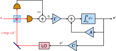
Figure 3: (Color online). A phase-locked loop that implements Kalman-Bucy filtering for angle demodulation.

For example, consider the message as an Ornstein-Uhlenbeck process,

$$\frac{dx}{dt} =-kx+Bu.$$ (47)

The variance equation becomes

$$\frac{d\Sigma}{dt} =-2k\Sigma-\frac{4\beta^{2}\mathcal{P}}{\hbar\omega_{0}}\Sigma^{2}+\kappa, \kappa \equiv B^{2}U,$$ (48)

and the gain is

$$\Gamma(t) =\frac{4\beta\mathcal{P}}{\hbar\omega_{0}}\Sigma(t).$$ (49)

The variance equation can be solved analytically,

$$\Sigma(t) =\Sigma_{\rm ss}\frac{\mu-\frac{\gamma/k+1}{\gamma/k-1}\exp[-2\gamma(t-t_{0})]}{\mu+\exp[-2\gamma(t-t_{0})]},$$ (50)

$$\mu \equiv\frac{\gamma/k+1+\Lambda\Sigma(t_{0})}{\gamma/k-1-\Lambda\Sigma(t_{0})},\quad\gamma\equiv k\left(\frac{\kappa\Lambda}{k}+1\right)^{1/2},$$

$$\Lambda \equiv\frac{4\beta^{2}\mathcal{P}}{\hbar\omega_{0}k}.$$ (51)

where the subscript ss denotes the steady state,

$$\Sigma(t) \to\Sigma_{\rm ss}\equiv\frac{1}{\Lambda}\left[\left(\frac{\kappa\Lambda}{k}+1\right)^{1/2}-1\right],\quad t-t_{0}\gg\frac{1}{\gamma},$$ (52)

$$\Sigma_{\rm ss} \approx\left(\frac{\kappa}{k\Lambda}\right)^{1/2},\quad\frac{\kappa\Lambda}{k}\gg 1,$$ (53)

and the threshold constraint is

$$\Lambda\gg\frac{\kappa}{k}\beta^{4}.$$ (54)

When the message is a Wiener random process,

$$\frac{dx}{dt} =Bu,$$ (55)

we can either follow the same procedure as before to derive the Kalman-Bucy filter, or take the results for the Ornstein-Uhlenbeck process to the limit $k\to 0$. Either way, assuming $\beta=1$ for simplicity, we find

$$\Sigma(t) =\Sigma_{\rm ss}\frac{\mu-\exp[-2\gamma(t-t_{0})]}{\mu+\exp[-2\gamma(t-t_{0})]},\quad\Gamma(t)=\frac{4\mathcal{P}}{\hbar\omega_{0}}\Sigma(t),$$ (56)

$$\Sigma_{\rm ss} =\frac{1}{2\sqrt{N}},\quad\mu\equiv\frac{1+2\sqrt{N}\Sigma(t_{0})}{1-2\sqrt{N}\Sigma(t_{0})},$$

$$\gamma \equiv 2\kappa\sqrt{N},\quad N\equiv\frac{\mathcal{P}}{\hbar\omega_{0}\kappa}.$$ (57)

At steady state,

$$\Sigma(t)\to\Sigma_{\rm ss} =\frac{1}{2\sqrt{N}}, \Gamma(t) \to 2\kappa\sqrt{N}, t-t_{0}\gg\frac{1}{\gamma}.$$ (58)

The threshold constraint is

$$4N=\frac{4\mathcal{P}}{\hbar\omega_{0}\kappa}\gg 1.$$ (59)

These results for the Wiener process agree with Berry and Wiseman’s berry .

III.2 Wiener filtering

In addition to the Kalman-Bucy state-variable approach, Wiener’s frequency-domain approach can also be used to design the phase-locked loop tsang ; vantrees ; viterbi . Defining

$$y(t) \equiv\bar{\phi}(t)+z(t),$$ (60)

it can be shown that Kalman-Bucy filtering is equivalent to the integral equation vantrees ; baggeroer

$$\boldsymbol{x}^{\prime}(t) =\int_{t_{0}}^{t}d\tau\boldsymbol{H}(t,\tau)y(\tau),$$ (61)

where $\boldsymbol{H}(t,\tau)$ is called the optimum realizable filter and satisfies the integral equation

$$\boldsymbol{K}_{xy}(t,\sigma) =\int_{t_{0}}^{t}d\tau\boldsymbol{H}(t,\tau)K_{y}(\tau,\sigma),$$ (62)

$$\boldsymbol{K}_{xy}(t,\sigma) \equiv\left\langle\boldsymbol{x}(t)y(\sigma)\right\rangle,\quad K_{y}(\tau,\sigma)=\left\langle y(\tau)y(\sigma)\right\rangle.$$ (63)

If $\boldsymbol{x}(t)$ and $y(t)$ are stationary and we let $t_{0}\to-\infty$, Eq. (62) becomes the Wiener-Hopf equation,

$$\boldsymbol{K}_{xy}(t-\sigma) =\int_{-\infty}^{t}d\tau\boldsymbol{H}(t-\tau)K_{y}(\tau-\sigma),$$ (64)

which can be solved by a well-known frequency-domain technique tsang ; vantrees ; viterbi . For example, if $x(t)$ is an Ornstein-Uhlenbeck process, its power spectral density in the limit of $t_{0}\to-\infty$ is

$$K_{x}(t,\sigma) \equiv\left\langle x(t)x(\sigma)\right\rangle=K_{x}(t-\sigma),$$ (65)

$$S_{x}(\omega) \equiv\int_{-\infty}^{\infty}dtK_{x}(t)\exp(-i\omega t)=\frac{\kappa}{\omega^{2}+k^{2}}.$$ (66)

The power spectral density for $y(t)$ is then

$$S_{y}(\omega) \equiv\int_{-\infty}^{\infty}dtK_{y}(t)\exp(-i\omega t)=\frac{\beta^{2}\kappa}{\omega^{2}+k^{2}}+\frac{\hbar\omega_{0}}{4\mathcal{P}}.$$ (67)

To solve for $H(t-\tau)$, we rewrite $S_{y}(\omega)$ as

$$S_{y}(\omega) =H_{+}(\omega)H_{+}^{*}(\omega), H_{+}(\omega) =\left(\frac{\hbar\omega_{0}}{4\mathcal{P}}\right)^{1/2}\frac{i\omega+\gamma}{i\omega+k},$$ (68)

where $\gamma$ is given in Eq. (51), and $H_{+}(\omega)$ and $1/H_{+}(\omega)$ are causal filters. Defining

$$S_{xy}(\omega) \equiv\int_{-\infty}^{\infty}dtK_{xy}(t)\exp(-i\omega t)=\frac{\beta\kappa}{\omega^{2}+k^{2}},$$ (69)

the Wiener filter in the frequency domain is

$$H(\omega) =\frac{1}{H_{+}(\omega)}\left[\frac{S_{xy}(\omega)}{H_{+}^{*}(\omega)}\right]_{+},$$ (70)

where the subscript $+$ denotes the realizable part. To calculate the realizable part, first perform the inverse Fourier transform,

$$\quad\int\frac{d\omega}{2\pi}\frac{S_{xy}(\omega)}{H_{+}^{*}(\omega)}\exp(i\omega t)$$

$$=\left(\frac{4\mathcal{P}}{\hbar\omega_{0}}\right)^{1/2}\frac{\beta\kappa}{\gamma+k}\left[\mathcal{U}(-t)e^{\gamma t}+\mathcal{U}(t)e^{-kt}\right],$$ (71)

where $\mathcal{U}(t)$ is the Heaviside step function. The realizable part is then obtained by multiplying Eq. (71) by $\mathcal{U}(t)$ and performing the Fourier transform. After some algebra, we obtain

$$H(\omega) =\frac{\Gamma_{\rm ss}}{i\omega+\gamma}, \Gamma_{\rm ss} \equiv\frac{\gamma-k}{\beta}.$$ (72)

To implement the Wiener filter in the phase-locked loop shown in Fig. 4, the loop filter that relates the homodyne output $\eta(t)$ to the estimate $x^{\prime}(t)$ is

$$x^{\prime}(t) =\int_{-\infty}^{t}d\tau L(t-\tau)\eta(\tau)$$ (73)

$$\approx\int_{-\infty}^{t}d\tau L(t-\tau)[y(\tau)-\beta x^{\prime}(\tau)],$$ (74)

$$\frac{L(\omega)}{1+\beta L(\omega)} =H(\omega),\quad L(\omega)=\frac{H(\omega)}{1-\beta H(\omega)}=\frac{\Gamma_{\rm ss}}{i\omega+k}.$$ (75)

The resulting phase-locked-loop structure is equivalent to that obtained by Kalman-Bucy filtering at steady state, as both approaches implement the optimum realizable filter.

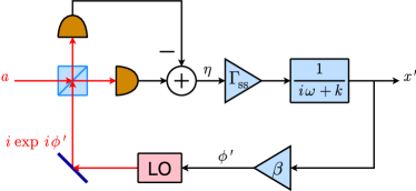
Figure 4: (Color online). A phase-locked loop implementation of Wiener filtering when the mean phase is an Ornstein-Uhlenbeck process.

The mean-square error of Wiener filtering is given by the well-known expression tsang ; vantrees ; viterbi

$$\Sigma =\frac{\hbar\omega_{0}}{4\beta^{2}\mathcal{P}}\int_{-\infty}^{\infty}\frac{d\omega}{2\pi}\ln\left[1+\frac{4\beta^{2}\mathcal{P}S_{x}(\omega)}{\hbar\omega_{0}}\right]$$

$$=\frac{1}{\Lambda}\left[\left(\frac{\kappa\Lambda}{k}+1\right)^{1/2}-1\right],$$ (76)

which obviously must be the same as the steady-state error $\Sigma_{\rm ss}$ obtained by Kalman-Bucy filtering. The interested reader is referred to Ref. vantrees for an excellent treatment of Wiener filters.

The advantage of Kalman-Bucy filtering over Wiener filtering is that the former can also deal with a wide class of nonstationary random processes that can be described by a system of linear equations (28), whereas Wiener filtering works only for stationary processes. In the special case of a Wiener process, however, we can first design a Wiener filter for an Ornstein-Uhlenbeck process and take the limit $k\to 0$. The result for $\beta=1$ is

$$L(\omega) \to\frac{\Gamma_{\rm ss}}{i\omega}, \Gamma_{\rm ss} \to 2\kappa\sqrt{N}, \Sigma \to\frac{1}{2\sqrt{N}},$$ (77)

which is again the same as the steady-state Kalman-Bucy filter.

IV Smoothing

Both Kalman-Bucy filtering and Wiener filtering provide real-time estimates of $\boldsymbol{x}(t)$ based on the measurement record up to time $\tau=t$. If we allow delay in the estimation, we can use the additional information from more advanced measurements to improve upon the estimation. In the following we consider the optimal estimation of $\boldsymbol{x}(t)$ given the full measurement record in the interval $t_{0}\leq t\leq T$, also called smoothing in classical estimation theory vantrees ; baggeroer .

IV.1 State-variable approach

Given the output $\boldsymbol{x}^{\prime}$ of the homodyne phase-locked loop designed by Kalman-Bucy filtering and the associated covariance matrix $\boldsymbol{\Sigma}$, the optimal smoothing estimates of $\boldsymbol{x}(t)$, which we define as $\widetilde{\boldsymbol{x}}(t)$, can be calculated using a state-variable approach, first suggested by Bryson and Frazier baggeroer ; rts . $\widetilde{\boldsymbol{x}}(t)$ and the smoothing covariance matrix,

$$\boldsymbol{\Pi}(t) \equiv\left\langle\left[\boldsymbol{x}(t)-\widetilde{\boldsymbol{x}}(t)\right]\otimes\left[\boldsymbol{x}(t)-\widetilde{\boldsymbol{x}}(t)\right]\right\rangle,$$ (78)

can be obtained by solving the following equations backward in time,

$$\frac{d\widetilde{\boldsymbol{x}}}{dt} =\boldsymbol{A}\widetilde{\boldsymbol{x}}+\boldsymbol{B}\boldsymbol{U}\boldsymbol{B}^{T}\boldsymbol{\Sigma}^{-1}\left(\widetilde{\boldsymbol{x}}-\boldsymbol{x}^{\prime}\right),$$ (79)

$$\frac{d\boldsymbol{\Pi}}{dt} =\left(\boldsymbol{A}+\boldsymbol{B}\boldsymbol{U}\boldsymbol{B}^{T}\boldsymbol{\Sigma}^{-1}\right)\boldsymbol{\Pi}+\boldsymbol{\Pi}\left(\boldsymbol{A}+\boldsymbol{B}\boldsymbol{U}\boldsymbol{B}^{T}\boldsymbol{\Sigma}^{-1}\right)^{T}$$

$$\quad-\boldsymbol{B}\boldsymbol{U}\boldsymbol{B}^{T},$$ (80)

with the final conditions,

$$\widetilde{\boldsymbol{x}}(T) =\boldsymbol{x}^{\prime}(T), \boldsymbol{\Pi}(T) =\boldsymbol{\Sigma}(T).$$ (81)

In the $t_{0}\ll t\ll T$ limit, we can calculate the steady-state smoothing covariance matrix $\boldsymbol{\Pi}_{\rm ss}$ by setting the right-hand side Eq. (80) to zero and using the steady-state $\boldsymbol{\Sigma}_{\rm ss}$ as $\boldsymbol{\Sigma}$.

Again using the Ornstein-Uhlenbeck process as an example, the steady-state smoothing error, also called the “irreducible” error vantrees ; viterbi , is given by

$$\Pi_{\rm ss} =\frac{\kappa}{2k(\kappa\Lambda/k+1)^{1/2}}.$$ (82)

This result is identical to that derived in tsang using a frequency-domain approach. In the limit of $\Lambda\gg k/\kappa$,

$$\Pi_{\rm ss} \to\frac{1}{2}\left(\frac{\kappa}{k\Lambda}\right)^{1/2}\approx\frac{1}{2}\Sigma_{\rm ss},$$ (83)

which is smaller than the error from Kalman-Bucy or Wiener filtering by approximately a factor of 2. For the Wiener process, the smoothing error is

$$\Pi_{\rm ss} =\frac{1}{4\sqrt{N}}=\frac{1}{2}\Sigma_{\rm ss},$$ (84)

which is smaller than the filtering error by exactly a factor of 2.

IV.2 Two-filter smoothing

An equivalent but more intuitive form of the optimal smoother was discovered by Mayne mayne and Fraser and Potter fraser , who treat the smoother as a combination of two filters, one running forward in time to produce a prediction $\boldsymbol{x}^{\prime}(t)$ via Kalman-Bucy filtering using the past measurement record, as specified by Eqs. (36) to (44), and one running backward in time to produce a retrodiction $\boldsymbol{x}^{\prime\prime}(t)$ using the advanced measurement record,

$$\frac{d\boldsymbol{x}^{\prime\prime}}{dt} =\boldsymbol{A}\boldsymbol{x}^{\prime\prime}-\boldsymbol{\Upsilon}\boldsymbol{\eta},$$ (85)

$$\frac{d\boldsymbol{\Xi}}{dt} =\boldsymbol{A}\boldsymbol{\Xi}+\boldsymbol{\Xi}\boldsymbol{A}^{T}+\boldsymbol{\Xi}\boldsymbol{C}^{T}\boldsymbol{Z}^{-1}\boldsymbol{C}\boldsymbol{\Xi}-\boldsymbol{B}\boldsymbol{U}\boldsymbol{B}^{T},$$ (86)

$$\boldsymbol{\Upsilon} =\boldsymbol{\Xi}\boldsymbol{C}^{T}\boldsymbol{Z}^{-1},$$ (87)

with final conditions

$$\boldsymbol{\Xi}^{-1}(T)\boldsymbol{x}^{\prime\prime}(T) =\boldsymbol{0}, \boldsymbol{\Xi}^{-1}(T)=\boldsymbol{0}.$$ (88)

The smoothing estimates and covariance matrix, taking into account both the prediction and the retrodiction, are given by

$$\widetilde{\boldsymbol{x}} =\boldsymbol{\Pi}\left(\boldsymbol{\Sigma}^{-1}\boldsymbol{x}^{\prime}+\boldsymbol{\Xi}^{-1}\boldsymbol{x}^{\prime\prime}\right),$$ (89)

$$\boldsymbol{\Pi} =\left(\boldsymbol{\Sigma}^{-1}+\boldsymbol{\Xi}^{-1}\right)^{-1}.$$ (90)

The steady-state smoothing covariance matrix $\boldsymbol{\Pi}_{\rm ss}$ can be calculated by combining the steady-state predictive and retrodictive covariance matrices,

$$\boldsymbol{\Pi}_{\rm ss} =\left(\boldsymbol{\Sigma}^{-1}_{\rm ss}+\boldsymbol{\Xi}^{-1}_{\rm ss}\right)^{-1}.$$ (91)

IV.3 Frequency-domain approach

For stationary Gaussian random processes and in the limit of $t_{0}\ll t\ll T$, a frequency-domain approach can also be used to obtain the optimal smoother tsang ; vantrees ; viterbi . The optimal smoothing estimates can be written in terms of $y(t)$ as vantrees ; baggeroer ; viterbi

$$\widetilde{\boldsymbol{x}}(t) =\int_{t_{0}}^{T}d\tau\boldsymbol{G}(t,\tau)y(\tau),$$ (92)

where $\boldsymbol{G}(t,\tau)$ obeys

$$\boldsymbol{K}_{xy}(t,\sigma) =\int_{t_{0}}^{T}d\tau\boldsymbol{G}(t,\tau)K_{y}(\tau,\sigma).$$ (93)

For $\boldsymbol{K}_{xy}(t,\sigma)=\boldsymbol{K}_{xy}(t-\sigma)$, $\boldsymbol{G}(t,\tau)=\boldsymbol{G}(t-\tau)$, and $K_{y}(\tau,\sigma)=K_{y}(\tau-\sigma)$, and in the limit of $t_{0}\to-\infty$ and $T\to\infty$, we can solve Eq. (93) by Fourier transform,

$$\boldsymbol{G}(\omega) =\frac{\boldsymbol{S}_{xy}(\omega)}{S_{y}(\omega)}.$$ (94)

$\boldsymbol{G}(\omega)$ is called the optimum unrealizable filter vantrees . For an Ornstein-Uhlenbeck process, $G(\omega)$ is

$$G(\omega) =\frac{4\beta\mathcal{P}}{\hbar\omega_{0}}\frac{\kappa}{\omega^{2}+\gamma^{2}}.$$ (95)

To implement this filter, one can use the homodyne phase-locked loop designed by Wiener filtering and a post-loop filter given by

$$F(\omega) =\frac{G(\omega)}{H(\omega)}=\frac{k+\gamma}{-i\omega+\gamma}.$$ (96)

The post-loop filter impulse response is

$$f(t) \equiv\int_{-\infty}^{\infty}\frac{d\omega}{2\pi}F(\omega)\exp(i\omega t)$$ (97)

$$=\Big{\{}\begin{array}[]{cc}(k+\gamma)\exp(\gamma t),&t\leq 0,\\ 0,&t>0,\end{array}$$ (100)

which is anti-causal, so one must introduce a time delay $t_{d}\gg 1/\gamma$ for $F$ to be approximated by a causal filter. The optimal smoother designed by the frequency-domain approach is depicted in Fig. 5.

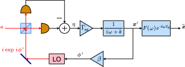
Figure 5: (Color online). A homodyne phase-locked loop with a post-loop filter $F(\omega)$ that realizes optimal smoothing.

The variance of the optimal frequency-domain smoother is tsang ; vantrees ; viterbi

$$\Pi =\int_{-\infty}^{\infty}\frac{d\omega}{2\pi}\left[S_{x}(\omega)-\frac{|S_{xy}(\omega)|^{2}}{S_{y}(\omega)}\right]$$

$$=\frac{\kappa}{2k(\kappa\Lambda/k+1)^{1/2}},$$ (101)

which is the same as the smoothing error derived by the state-variable approach in Eq. (82), as expected. The interested reader is again referred to Ref. vantrees for an excellent treatment of optimal frequency-domain filters and smoothers.

V Quantum position and momentum estimation by optical phase measurements

V.1 Quantum Kalman-Bucy filtering

So far we have assumed that the mean phase of the optical field contains classical random processes to be estimated in the presence of quantum optical noise. In this section we investigate the estimation of inherently quantum processes carried by the optical phase. Specifically, we revisit the classic problem of quantum-limited mirror position and momentum estimation by optical phase measurements. First we review the problem of optimal real-time estimation by Kalman-Bucy filtering, previously studied by Belavkin and Staszewski belavkin and Doherty et al. doherty .

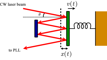
Figure 6: (Color online). Position and momentum estimation by optical phase measurements.

We model the mirror as a harmonic oscillator, as depicted in Fig. 6,

$$\frac{d\hat{x}}{dt} =\frac{\hat{p}}{m},$$ (102)

$$\frac{d\hat{p}}{dt} =-m\omega_{m}^{2}\hat{x}+\frac{2M\hbar\omega_{0}\cos\theta}{c}\hat{I},$$ (103)

where $\hat{x}(t)$ and $\hat{p}(t)$ are quantum position and momentum operators, $m$ is the harmonic-oscillator mass, $\omega_{m}$ is the mechanical harmonic-oscillator frequency, the last term of Eq. (103) is the radiation pressure term, $M$ is the number of times the optical beam hits the mirror, $\theta$ is the angle at which the optical beam hits the mirror, and $\hat{I}(t)$ is the optical flux operator, consisting of a mean and a quantum noise term,

$$\hat{I}(t) =\frac{\mathcal{P}}{\hbar\omega_{0}}+\Delta\hat{I}(t).$$ (104)

The constant force term can be eliminated by redefining the position of the harmonic oscillator, so we shall neglect the constant radiation pressure term from now on. $\Delta\hat{I}(t)$ is approximately a white Gaussian noise term for a high-power optical coherent state,

$$\left\langle\Delta\hat{I}(t)\Delta\hat{I}(\tau)\right\rangle \approx\frac{\mathcal{P}}{\hbar\omega_{0}}\delta(t-\tau).$$ (105)

The Gaussian approximation neglects the discreteness of photon number, and is valid if the number of photons within the relaxation time of the filter impulse response is much larger than 1. We can then write the quantum system model as

$$\frac{d}{dt}\left[\begin{array}[]{c}\hat{x}\\ \hat{p}\end{array}\right] =\left[\begin{array}[]{cc}0&1/m\\ -m\omega_{m}^{2}&0\end{array}\right]\left[\begin{array}[]{c}\hat{x}\\ \hat{p}\end{array}\right]+\left[\begin{array}[]{c}0\\ 1\end{array}\right]\hat{u},$$ (114)

with initial conditions

$$\langle\hat{x}(t_{0})\rangle =0, \langle\hat{p}(t_{0})\rangle =0,$$ (115)

and radiation pressure acting as the quantum Langevin noise,

$$\left\langle\hat{u}(t)\hat{u}(\tau)\right\rangle=U\delta(t-\tau),$$ (116)

$$U\equiv\frac{\hbar\beta^{2}\mathcal{P}}{\omega_{0}},\quad\beta\equiv 2Mk_{0}\cos\theta.$$ (117)

The mirror position is observed via optical phase measurements using a phase-locked loop. In the linearized regime, we can define the quantum observation process as

$$\hat{y} =\left[\begin{array}[]{cc}\beta&0\end{array}\right]\left[\begin{array}[]{c}\hat{x}\\ \hat{p}\end{array}\right]+\hat{z},$$ (121)

$$\left\langle\hat{z}(t)\hat{z}(\tau)\right\rangle =Z\delta(t-\tau),\quad Z\equiv\frac{\hbar\omega_{0}}{4\mathcal{P}}.$$ (122)

Our linearized model is consistent with the general model of continuous quantum non-demolition (QND) measurements belavkin ; doherty ; caves .

To apply Kalman-Bucy filtering to the estimation of mirror position and momentum, let us define

$$\Delta\hat{x} \equiv\hat{x}-x^{\prime},\quad\Delta\hat{p}\equiv\hat{p}-p^{\prime},$$ (123)

$$\boldsymbol{\Sigma} =\left[\begin{array}[]{cc}\langle\Delta\hat{x}^{2}\rangle&\frac{1}{2}\left\langle\Delta\hat{x}\Delta\hat{p}+\Delta\hat{p}\Delta\hat{x}\right\rangle\\ \frac{1}{2}\langle\Delta\hat{x}\Delta\hat{p}+\Delta\hat{p}\Delta\hat{x}\rangle&\langle\Delta\hat{p}^{2}\rangle\end{array}\right].$$ (126)

In the linearized model, the Wigner distribution remains Gaussian and non-negative provided that the initial Wigner distribution is Gaussian, so it can be regarded as a classical phase-space probability distribution, $\hat{x}(t)$, $\hat{p}(t)$, $\Delta\hat{I}(t)$, and $\hat{y}(t)$ can be regarded as classical random processes with statistics governed by the Wigner distribution, and we can apply classical estimation theory directly. The off-diagonal components of the variance matrix are written in terms of symmetrized operators to ensure that they are Hermitian and also obey Wigner-distribution statistics.

The Kalman-Bucy variance equations hence become

$$\frac{d\Sigma_{11}}{dt} =\frac{1}{m}(\Sigma_{21}+\Sigma_{12})-V\Sigma_{11}^{2},$$ (127)

$$\frac{d\Sigma_{12}}{dt} =\frac{1}{m}\Sigma_{22}-m\omega_{m}^{2}\Sigma_{11}-V\Sigma_{11}\Sigma_{12},$$ (128)

$$\frac{d\Sigma_{22}}{dt} =-m\omega_{m}^{2}(\Sigma_{12}+\Sigma_{21})-V\Sigma_{12}\Sigma_{21}+U,$$ (129)

$$V \equiv\frac{4\beta^{2}\mathcal{P}}{\hbar\omega_{0}}.$$ (130)

The steady state is given by the condition $d\boldsymbol{\Sigma}/dt=0$. After some algebra,

$$(\Sigma_{11})_{\rm ss} =\frac{\hbar}{2m\omega_{m}}\frac{\sqrt{2}}{Q}\left[\left(1+Q^{2}\right)^{1/2}-1\right]^{1/2},$$ (131)

$$(\Sigma_{12})_{\rm ss} =(\Sigma_{21})_{\rm ss}=\frac{\hbar}{2}\frac{1}{Q}\left[\left(1+Q^{2}\right)^{1/2}-1\right],$$ (132)

$$(\Sigma_{22})_{\rm ss} =\frac{\hbar m\omega_{m}}{2}\frac{\sqrt{2}}{Q}\left[\left(1+Q^{2}\right)^{1/2}-1\right]^{1/2}\left(1+Q^{2}\right)^{1/2},$$ (133)

where

$$Q \equiv\frac{\sqrt{UV}}{m\omega_{m}^{2}}=\frac{2\beta^{2}\mathcal{P}}{m\omega_{0}\omega_{m}^{2}}$$ (134)

is a dimensionless parameter that characterizes the strength of the measurements. The position uncertainty $\langle\Delta\hat{x}^{2}\rangle_{\rm ss}=(\Sigma_{11})_{\rm ss}$ is squeezed due to the continuous QND measurements, while the momentum uncertainty $\langle\Delta\hat{p}^{2}\rangle_{\rm ss}=(\Sigma_{22})_{\rm ss}$ is anti-squeezed due to the radiation pressure. These results have also been derived by various groups of people belavkin ; doherty , although here we have shown how one can realistically implement the optical measurements of a mechanical oscillator.

The Kalman-Bucy gain is

$$\boldsymbol{\Gamma} =\frac{4\beta\mathcal{P}}{\hbar\omega_{0}}\left[\begin{array}[]{c}\Sigma_{11}\\ \Sigma_{21}\end{array}\right].$$ (137)

The estimator equation becomes

$$\frac{d}{dt}\left[\begin{array}[]{c}x^{\prime}\\ p^{\prime}\end{array}\right] =\left[\begin{array}[]{cc}-V\Sigma_{11}&1/m\\ -V\Sigma_{21}-m\omega_{m}^{2}&0\end{array}\right]\left[\begin{array}[]{c}x^{\prime}\\ p^{\prime}\end{array}\right]$$ (144)

$$\quad+\frac{V}{\beta}\left[\begin{array}[]{c}\Sigma_{11}\\ \Sigma_{21}\end{array}\right]y,$$ (147)

where $y$ is the measurement record of $\hat{y}$. The filter relaxation time is on the order of

$$t_{f} \sim\frac{1}{V(\Sigma_{11})_{\rm ss}}=\frac{1}{\sqrt{2}\omega_{m}[(1+Q^{2})^{1/2}-1]^{1/2}},$$ (148)

which decreases for increasing $Q$, so the steady state can be reached faster for a larger $Q$. For $Q\to 0$, $t_{f}\to\infty$, and a steady state does not exist. The photon number within the filter relaxation time is much larger than 1, and the assumption of white Gaussian radiation pressure noise is valid, when

$$\frac{\mathcal{P}t_{f}}{\hbar\omega_{0}} \sim\frac{m\omega_{m}}{2\sqrt{2}\beta^{2}\hbar}\frac{Q}{[(1+Q^{2})^{1/2}-1]^{1/2}}\gg 1.$$ (149)

On the other hand, the threshold constraint, which ensures that the linearized analysis of the phase-locked loop is valid, is

$$\beta^{2}(\Sigma_{11})_{\rm ss} =\frac{\beta^{2}\hbar}{\sqrt{2}m\omega_{m}}\frac{[(1+Q^{2})^{1/2}-1]^{1/2}}{Q}\ll 1.$$ (150)

This condition, apart from a factor of $4$, is the same as the large-photon-number assumption given by Eq. (149), and ensures that the linearized system and measurement model is self-consistent.

The mirror position-momentum uncertainty product at steady state is

$$\langle\Delta\hat{x}^{2}\rangle_{\rm ss}\langle\Delta\hat{p}^{2}\rangle_{\rm ss} =(\Sigma_{11}\Sigma_{22})_{\rm ss}$$

$$=\frac{\hbar^{2}}{4}\frac{2}{Q^{2}}\left[1+Q^{2}-\left(1+Q^{2}\right)^{1/2}\right],$$ (151)

and satisfies the Heisenberg uncertainty principle for all $Q$, as one would expect. Furthermore, the covariances satisfy the following relation for pure Gaussian states belavkin ; doherty :

$$\operatorname{det}(\boldsymbol{\Sigma}_{\rm ss})=\left(\Sigma_{11}\Sigma_{22}-\Sigma_{12}^{2}\right)_{\rm ss}=\frac{\hbar^{2}}{4},$$ (152)

indicating that the harmonic oscillator conditioned upon the real-time measurement record becomes a pure Gaussian state at steady state.

V.2 Smoothing errors

From the classical estimation theory perspective, we should be able to improve upon Kalman-Bucy filtering if we allow delay in the estimation and apply smoothing. Here we calculate the steady-state smoothing errors using the two-filter approach described in Sec. IV.2. The steady-state smoothing covariance matrix is

$$\boldsymbol{\Pi}_{\rm ss} =\left(\boldsymbol{\Sigma}_{\rm ss}^{-1}+\boldsymbol{\Xi}_{\rm ss}^{-1}\right)^{-1},$$ (153)

where $\boldsymbol{\Sigma}_{\rm ss}$ is the steady-state forward-filter covariance matrix, already solved and given by Eqs. (131)–(133). The backward-filter covariances obey the following equations:

$$\frac{d\Xi_{11}}{dt} =\frac{1}{m}(\Xi_{21}+\Xi_{12})+V\Xi_{11}^{2},$$ (154)

$$\frac{d\Xi_{12}}{dt} =\frac{1}{m}\Xi_{22}-m\omega_{m}^{2}\Xi_{11}+V\Xi_{11}\Xi_{12},$$ (155)

$$\frac{d\Xi_{22}}{dt} =-m\omega_{m}^{2}(\Xi_{12}+\Xi_{21})+V\Xi_{12}\Xi_{21}-U.$$ (156)

The steady-state values for the backward filter turn out to be almost identical to the ones for the forward filter,

$$(\Xi_{11})_{\rm ss} =(\Sigma_{11})_{\rm ss}, (\Xi_{12})_{\rm ss} =-(\Sigma_{12})_{\rm ss},$$

$$(\Xi_{22})_{\rm ss} =(\Sigma_{22})_{\rm ss},$$ (157)

and also satisfy the pure-Gaussian-state relation

$$\operatorname{det}(\boldsymbol{\Xi}_{\rm ss})=\left(\Xi_{11}\Xi_{22}-\Xi_{12}^{2}\right)_{\rm ss}=\frac{\hbar^{2}}{4}.$$ (158)

After some algebra,

$$(\Pi_{11})_{\rm ss} =\frac{\hbar}{8m\omega_{m}}\left[\frac{1}{(1+iQ)^{1/2}}+\frac{1}{(1-iQ)^{1/2}}\right],$$ (159)

$$(\Pi_{12})_{\rm ss} =0,$$ (160)

$$(\Pi_{22})_{\rm ss} =\frac{\hbar m\omega_{m}}{8}\left[(1+iQ)^{1/2}+\left(1-iQ\right)^{1/2}\right].$$ (161)

These results can be confirmed using the frequency-domain approach outlined in Sec. IV.3. The position-momentum uncertainty product becomes

$$(\Pi_{11})_{\rm ss}(\Pi_{22})_{\rm ss}=\frac{\hbar^{2}}{32}\left[1+\frac{1}{(1+Q^{2})^{1/2}}\right],$$ (162)

which is smaller than the Heisenberg uncertainty product $\hbar^{2}/4$ by 4 to 8 times.

V.3 Discussion

While counter-intuitive, the sub-Heisenberg uncertainties given by Eqs. (159)–(162) do not violate any basic law of quantum mechanics. The reason is that we only estimate the position and momentum of the mirror some time in the past as if they were classical random processes with Wigner-distribution statistics, but it is impossible to verify our estimates by comparing them against the mirror in the past, which has since been irreversibly perturbed by the unknown radiation pressure noise. In classical estimation, $x(t)$ and $p(t)$ are classical random processes unknown to the observer but can in principle be perfectly measured or simply decided at will by another party, so it is possible to compare one’s delayed estimates against the perfect versions and verify the smoothing errors. In the quantum regime, however, one cannot measure the mirror in the past more accurately without disturbing it further, and the only way for us to obtain perfect information about the mirror position or momentum is to perform a strong projective measurement. Unlike the Kalman-Bucy estimates, which predict the mirror position and momentum at present and can be verified by performing a projective measurement at present, it is obviously impossible to go back to the past and perform a strong projective measurement on the mirror to verify our delayed estimates without changing our model of the problem.

It is also impossible to perfectly reverse the dynamics of the mirror in time and recreate the past quantum state without introducing additional noise, because quantum-limited optical phase measurements prevent us from obtaining any information about the optical power fluctuations, and the dynamics of the mirror subject to the unknown radiation pressure noise is irreversible. Thus, even though classical estimation theory indicates that we can achieve more accurate estimates than the Heisenberg uncertainty principle would allow, quantum mechanics seem to forbid one from experimentally verifying the violation. In this sense the apparent paradox is analogous to the Einstein-Podolsky-Rosen paradox epr and may yet have implications for the interpretation of quantum mechanics.

In practice, while one may argue from a frequentist point of view that delayed estimation of quantum processes is meaningless if it cannot be verified, smoothing should still be able to improve the estimation of a classical random process in a quantum system, such as a classical force acting on a quantum harmonic oscillator thorne .

VI Conclusion

In conclusion, we have used classical estimation theory to design homodyne phase-locked loop for quantum optical phase estimation, and shown that the estimation performance can be improved when delay is permitted and smoothing is applied. We have focused on coherent states, as it can be regarded as a classical field with additive phase-insensitive noise upon homodyne detection, and classical estimation techniques can be applied directly. The optimal adaptive homodyne measurement scheme for nonclassical states remains an open problem. Along this direction Berry and Wiseman have recently suggested the use of Bayesian estimation for narrowband squeezed states when the mean phase is a Wiener process berry2 . Generalization of their scheme to more general random processes is challenging but may be facilitated by classical nonlinear estimation techniques vantrees ; baggeroer .

When we apply the same classical techniques to the quantum-limited estimation of harmonic-oscillator position and momentum, we find that the two conjugate variables can be simultaneously estimated with inferred accuracies beyond the Heisenberg uncertainty relation, if smoothing is performed. Although quantum mechanics seems to forbid one from verifying the delayed estimates by destroying the evidence, this result remains counter-intuitive and may have implications for the interpretation of quantum mechanics. In the general context of quantum trajectory theory carmichael , quantum smoothing deserves further investigation and should be useful for quantum sensing and communication applications thorne ; barnett .

References

- (1) M. Tsang, J. H. Shapiro, and S. Lloyd, Phys. Rev. A78, 053820 (2008).
- (2) H. M. Wiseman, Phys. Rev. Lett. 75, 4587 (1995).
- (3) M. A. Armen, J. K. Au, J. K. Stockton, A. C. Doherty, and H. Mabuchi, Phys. Rev. Lett. 89, 133602 (2002).
- (4) D. W. Berry and H. M. Wiseman, Phys. Rev. A65, 043803 (2002).
- (5) D. T. Pope, H. M. Wiseman, and N. K. Langford, Phys. Rev. A70, 043812 (2004).
- (6) H. L. Van Trees, Detection, Estimation, and Modulation Theory, Part I (Wiley, New York, 2001); Detection, Estimation, and Modulation Theory, Part II: Nonlinear Modulation Theory (Wiley, New York, 2002).
- (7) A. B. Baggeroer, State Variables and Communication Theory (MIT Press, Cambridge, 1970).
- (8) V. P. Belavkin and P. Staszewski, Phys. Lett. A 140, 359 (1989).
- (9) A. C. Doherty, S. M. Tan, A. S. Parkins, and D. F. Walls, Phys. Rev. A60, 2380 (1999).
- (10) M. Tsang, J. H. Shapiro, and S. Lloyd, in Proceedings of the Ninth International Conference on Quantum Communication, Measurement and Computing (QCMC), edited by A. Lvovsky, AIP Conf. Proc. No. 1110 (AIP, Melville, 2009), pp. 29-32.
- (11) R. L. Hudson and K. R. Parthasarathy, Commun. Math. Phys. 93, 301 (1984); A. Barchielli, Quantum Opt. 2, 423 (1990); J. H. Shapiro, Quantum Semiclass. Opt. 10, 567 (1998).
- (12) A. J. Viterbi, Principles of Coherent Communication (McGraw-Hill, New York, 1966).
- (13) A. E. Bryson and M. Frazier, Proceedings of Optimum Synthesis Conference, Wright-Patterson Air Force Base, Ohio, Aeronautical Systems Division TDR-63-119, 353 (1962); H. E. Rauch, F. Tung, and C. T. Striebel, AIAA J. 3, 1445 (1965).
- (14) D. Q. Mayne, Automatica 4, 73 (1966).
- (15) D. C. Fraser and J. E. Potter, IEEE Trans. Automatic Control 14, 387 (1969); see also J. E. Wall, Jr., A. S. Willsky, and N. R. Sandell Jr., Stochastics 5, 1 (1981).
- (16) C. M. Caves and G. J. Milburn, Phys. Rev. A36, 5543 (1987).
- (17) A. Einstein, B. Podolsky, and N. Rosen, Phys. Rev. 47, 777 (1935).
- (18) C. M. Caves, K. S. Thorne, R. W. P. Derver, V. D. Sandberg, and M. Zimmermann, Rev. Mod. Phys. 52, 341 (1980); A. Barchielli, Phys. Rev. D32, 347 (1985).
- (19) D. W. Berry and H. M. Wiseman, Phys. Rev. A73, 063824 (2006).
- (20) V. P. Belavkin, Rep. Math. Phys. 43, A405 (1999); H. Carmichael, An Open Systems Approach to Quantum Optics (Springer-Verlag, Berlin, 1993); C. W. Gardiner and P. Zoller, Quantum Noise (Springer-Verlag, Berlin, 2000); and references therein.
- (21) S. M. Barnett, D. T. Pegg, J. Jeffers, and O. Jedrkiewicz, Phys. Rev. Lett. 86, 2455 (2001); M. Yanagisawa, e-print arXiv:0711.3885.