Likelihood-based inference for max-stable processes

Abstract

The last decade has seen max-stable processes emerge as a common tool for the statistical modelling of spatial extremes. However, their application is complicated due to the unavailability of the multivariate density function, and so likelihood-based methods remain far from providing a complete and flexible framework for inference. In this article we develop inferentially practical, likelihood-based methods for fitting max-stable processes derived from a composite-likelihood approach. The procedure is sufficiently reliable and versatile to permit the simultaneous modelling of joint and marginal parameters in the spatial context at a moderate computational cost. The utility of this methodology is examined via simulation, and illustrated by the analysis of U.S. precipitation extremes.

Keywords: Composite likelihood; Extreme value theory; Max-stable processes; Pseudo-likelihood, Rainfall; Spatial Extremes.

1 Introduction

A common objective of spatial analysis is to quantify and characterise the behavior of environmental phenomena such as precipitation levels, windspeed or daily temperatures. A number of generic approaches to spatial modelling have been developed (e.g. Barndorff-Nielsen et al., (1998); Cressie, (1993); Ripley, (2004)), but these are not necessarily ideal for handling extremal aspects given their focus on mean process levels. Analyses of spatial extremes are useful devices for understanding and predicting extreme events such as hurricanes, storms and floods. In light of recent concerns over climate change, the use of robust mathematical and statistical methods for such analyses has grown in importance

While the theory and statistical practice of univariate extremes is well developed, there is much less guidance for the modelling of spatial extremes. This is problematic as many environmental processes have a natural spatial domain. We consider a temporal series of componentwise maxima of process measurements recorded at $k=1,\ldots,K$ locations, within a contiguous region. Observations $\{y_{n,k}\}$ each denote the maximum of $m$ samples over $n=1,\ldots,N$ temporal blocks. For example, for daily observations, $m=366$ implies the $\{y_{n,k}\}$ describe process annual maxima.

The spatial analogue of multivariate extreme value models is the class of max-stable processes (de Haan,, 1984; de Haan and Pickands,, 1986; Resnick,, 1987). Max-stable processes have a similar asymptotic motivation to the univariate Generalised Extreme Value (GEV) (von Mises,, 1954; Jenkinson,, 1955)), providing a general approach to modelling process extremes incorporating temporal or spatial dependence. Statistical methods for max-stable processes and data analysis of practical problems are discussed by Smith, (1990), Coles, (1993), Coles and Walshaw, (1994) and Coles and Tawn, (1996). Standard likelihood methods for such models are complicated by the intractability of the multivariate density function in all but the most trivial cases. This presents an obstacle in the use of max-stable processes for spatial extremes.

There is a lack of a proper inferential framework for the analysis of spatial extremes (although De Haan and Pereira, (2006) describe some non-parametric estimators). In this article we develop flexible and inferentially practical methods for the fitting of max-stable processes to spatial data based on non-standard, composite likelihood-based methods Lindsay, (1988). An appealing feature of this approach is that the estimation of GEV marginal parameters can be performed jointly with the dependence parameters in a unified framework. Accordingly, there is no need for separate estimation procedures. With highly-structured problems such as max-stable processes, this approach produces flexible and reliable results with a moderate computational cost.

The article is organised as follows: Section 2 reviews the theory of max-stable processes and its relationship to spatial extremes. Our composite likelihood approach is developed in Section 3 and Section 4 evaluates the method’s performance through a number of simulation studes. We conclude with an illustration of a real extremal data analysis of U.S. precipitation levels.

2 Max-stable processes and spatial extremes

2.1 Max-stable processes

Max-stable processes provide a natural generalisation of extremal dependence structures in continuous spaces. From this, closed-form bivariate distributions can be derived.

Definition.  Let $T$ be an index set and $\{\tilde{Y}_{i}(t)\}_{t\in T}$, $i=1,\ldots,n$ be $n$ independent replications of a continuous stochastic process. Assume that there are sequences of continuous functions $a_{n}(t)>0$ and $b_{n}(t)\in\mathbb{R}$ such that

$$Y(t)=\lim_{n\rightarrow\infty}\frac{\max_{i=1}^{n}\tilde{Y}_{i}(t)-b_{n}(t)}{a_{n}(t)},\quad t\in T.$$

If this limit exists, the limit process $Y(t)$ is a max-stable process de Haan, (1984).

Two properties follow from the above definition De Haan and Resnick, (1977). Firstly, the one-dimensional marginal distributions belong to the class of generalised extreme value distributions (GEV), $Y\sim\text{GEV}(\mu,\lambda,\xi)$ with distribution function

$$F(y;\mu,\lambda,\xi)=\exp\left[-\left\{1+\frac{\xi(y-\mu)}{\lambda}\right\}_{+}^{-1/\xi}\right],\quad-\infty<\mu,\quad\xi<\infty,\quad\lambda>0,$$

where $a_{+}=\max(0;a)$ and $\mu$, $\lambda$ and $\xi$ are respectively location, scale and shape parameters Fisher and Tippett, (1928). Secondly, for any $K=2,3,\ldots$, the $K$-dimensional marginal distribution belongs to the class of multivariate extreme value distributions.

W.l.o.g. if $a_{n}(t)=n$, $b_{n}(t)=0$ $\forall t$, then the corresponding process, $\{Z(t)\}_{t\in T}$, has unit Fréchet margins, with distribution function $F(z)=\exp(-1/z),z>0.$ This process is obtainable as standardisation of $\{Y(t)\}_{t\in T}$ through

$$\{Z(t)\}_{t\in T}\equiv\left[\left\{1+\frac{\xi(t)(Y(t)-\mu(t))}{\lambda(t)}\right\}_{+}^{1/\xi(t)}\right]_{t\in T},$$

where $\mu(t)$, $\xi(t)$ and $\lambda(t)>0$ are now continuous functions. The process $Z$ is still a max-stable process. If $Z$ is also stationary, the process may be expressed through it’s spectral representation de Haan and Pickands, (1986).

In detail, let $\{X_{j},U_{j}\}_{j\geq 1}$ be a Poisson process, $\Pi$, on $\mathbb{R}^{n}\times\mathbb{R}_{+}$, with counting measure $\Pi(\cdot):=\Sigma_{j}\mathbb{I}_{(X_{j},U_{j})}(\cdot)$ and intensity measure $\nu(dx)\times u^{-2}du$, where $\mathbb{I}_{(X_{j},U_{j})}(A)$ is the indicator function of the random number of points falling in a bounded set $A\subset\mathbb{R}^{n}\times\mathbb{R}_{+}$ and $\nu$ is a positive measure. For a nonnegative measurable (for fixed $t\in T$) function $f(x-t)$ such that $\int_{\mathbb{R}^{n}}f(x-t)\nu(dx)=1,\forall t\in T$ the stochastic process

$$Z(t):=\max_{j=1,2,\dots}\{U_{j}f(X_{j}-t)\},\quad t\in T,$$ (1)

is a stationary max-stable process de Haan, (1984). Smith, (1990) reinterprets this process in terms of environmental episodes such as storm phenomena, in which $U$, $X$ and $f$ represent respectively storm magnitude, the center and the shape. Schlather and Tawn, (2003) term this the storm profile model.

For a finite set of indexes $t_{1},\ldots,t_{K}\in T$ and positive thresholds $z_{1},\ldots,z_{K}$ for $K\in\mathbb{N}$, the distribution of the random vector $Z(t_{1}),\ldots,Z(t_{K})$ is de Haan, (1984)

$$\Pr\{Z(t_{k})\leq z_{k},\,k=1,\ldots,K\}=\exp\left[-\int_{\mathbb{R}^{n}}\max_{1\leq k\leq K}\left\{\frac{f(x-t_{k})}{z_{k}}\right\}\nu(dx)\right].$$ (2)

It then follows that the marginal distributions are unit Fréchet:

$$\Pr\{Z(t)\leq z\}=\exp\left(-z^{-1}\int_{\mathbb{R}^{n}}f(x-t)\nu(dx)\right)=\exp(-1/z).$$

Alternative spectral representations of max-stable processes exist (Schlather,, 2002).

2.2 Extremal coefficients

Given $n$ independent realisations of a random vector $Y\in\mathbb{R}^{d}$, the joint distribution of componentwise maxima satisfies (De Haan and Resnick,, 1977; Resnick,, 1987)

$$\Pr\left\{\max_{k}\max_{j=1,\ldots,n}Y_{k}^{(j)}/n\leq z\right\}=\Pr\left\{\max_{j=1,\ldots,n}Y_{1}^{(j)}/n\leq z\right\}^{\theta}=\exp(-\theta/z),\quad z>0,$$

for $k=1,2,\dots,K$ and common threshold $z$, where the rightmost term is a Fréchet$(\theta)$ distribution. The parameter $1\leq\theta\leq K$ is the extremal coefficient and it measures the extremal dependence between the margins, an important practical quantity in applications Smith, (1990). The information in the extremal coefficient reflects the practical number of independent variables. If $K$ is finite then $\theta=1$ indicates complete dependence, whereas $\theta=K$ demonstrates full independence.

In the max-stable process framework, from (2), for all $z>0$ we have

$$\Pr\{Z(t_{k})\leq z,\,k=1,\ldots,K\}=\exp(-\theta/z),$$

and so

$$\theta=\int_{\mathbb{R}^{n}}\max_{1\leq k\leq K}\left\{f(x-t_{k})\right\}\nu(dx).$$

where $\theta$ again represents the effective number of independent variables. Schlather and Tawn, (2003) discuss the extremal coefficient within a max-stable context.

2.3 Spatial models

Suppose now that $T\subseteq\mathbb{R}^{2}$ and that $\{X_{j}\}_{j\geq 1}$ are random points in $\mathbb{R}^{2}$. While for $K>2$, the general $K$-dimensional distribution function under the max-stable process representation (1) permits no analytically tractable form, a class of bivariate spatial models is available when the storm profile model, $f$, is a bivariate Gaussian density and $\mu$ is a Lebesgue measure (Smith,, 1990; De Haan and Pereira,, 2006). In this case, for locations ${\bf t}_{i}$ and ${\bf t}_{j}$ the bivariate distribution function of $\{Z({\boldsymbol{0}}),Z({\bf h})\}$ is

$$\begin{split}&\Pr\{Z({\boldsymbol{0}})\leq z_{i},Z({\bf h})\leq z_{j}\}\\ &=\exp\bigg{[}-\frac{1}{z_{i}}\Phi\left(\frac{a({\bf h})}{2}+\frac{1}{a({\bf h})}\log\frac{z_{j}}{z_{i}}\right)-\frac{1}{z_{j}}\Phi\left(\frac{a({\bf h})}{2}+\frac{1}{a({\bf h})}\log\frac{z_{i}}{z_{j}}\right)\bigg{]},\end{split}$$ (3)

where ${\bf h}=({\bf t}_{j}-{\bf t}_{i})^{\top}$, ${\boldsymbol{0}}$ is the origin, $\Phi$ is the standard Gaussian distribution function, $a({\bf h})=({\bf h}^{T}{\hbox{\hbox to0.0pt{$\Sigma$\hss}\kern 0.25pt\hbox to0.0pt{$\Sigma$\hss}\kern 0.25pt$\Sigma$}}^{-1}{\bf h})^{1/2}$ and $\Sigma$$\Sigma$$\Sigma$ is the covariance matrix of $f$, with covariance $\sigma_{12}$ and standard deviations $\sigma_{1},\sigma_{2}>0$. A derivation of (3) is in Appendix A.2. A general max-stable process with a Gaussian storm profile model, $f$, is termed a Gaussian extreme value process Smith, (1990), whereas the specific model (3) is the Gaussian extreme value model Coles, (1993).

Second-order partial derivatives of (3) yield the 2-dimensional density function

$$\begin{split}f(z_{i},z_{j})&=\exp\bigg{\{}-\frac{\Phi(w({\bf h}))}{z_{i}}-\frac{\Phi(v({\bf h}))}{z_{j}}\bigg{\}}\Bigg{\{}\left(\frac{\Phi(w({\bf h}))}{z_{i}^{2}}+\frac{\varphi(w({\bf h}))}{a({\bf h})z_{i}^{2}}-\frac{\varphi(v({\bf h}))}{a({\bf h})z_{i}z_{j}}\right)\\ &\bigg{(}\frac{\Phi(v({\bf h}))}{z_{j}^{2}}+\frac{\varphi(v({\bf h}))}{a({\bf h})z_{j}^{2}}-\frac{\varphi(w({\bf h}))}{a({\bf h})z_{i}z_{j}}\bigg{)}+\bigg{(}\frac{v({\bf h})\,\varphi(w({\bf h}))}{a({\bf h})^{2}z_{i}^{2}z_{j}}+\frac{w({\bf h})\,\varphi(v({\bf h}))}{a({\bf h})^{2}z_{i}z_{j}^{2}}\bigg{)}\Bigg{\}},\end{split}$$ (4)

where $\varphi$ is the standard Gaussian density function, $w({\bf h})=a({\bf h})/2+\log(z_{j}/z_{i})/a({\bf h})$ and $v({\bf h})=a({\bf h})-w({\bf h})$. The derivation of (4) is in Appendix A.3.

Observe that $a({\bf h})$ measures the strength of extremal dependence: $a({\bf h})\rightarrow 0$ represents complete dependence, and (in the limit) $a(h)\rightarrow\infty$ indicates complete independence. In accordance with spatial models, the extreme dependence between $Z({\boldsymbol{0}})$ and $Z({\bf h})$ decreases monotonically and continuously with ${\bf h}=\|{\bf t}_{j}-{\bf t}_{i}\|$ De Haan and Pereira, (2006), and for fixed ${\bf h}$ the dependence decreases monotonically as $a({\bf h})$ increases. Accordingly, characterisation of extremal dependence is determined by the covariance, $\Sigma$$\Sigma$$\Sigma$, which is therefore of interest for inference.

Due to high-dimensional distributional complexity the study of extremal dependence is commonly limited to pairwise components through the extremal coefficients

$$\theta({\bf h})=\int_{\mathbb{R}^{2}}\max\{f({\bf x}),f({\bf x}-{\bf h})\}d{\bf x},\qquad 1\leq\theta({\bf h})\leq 2.$$

The dependence on ${\bf h}$ is explicit. Specifically for the Gaussian extreme value model, $\theta({\bf h})=2\Phi(a({\bf h})/2),$ following an argument along the lines of Appendix A.2. Alternative models result by considering e.g. exponential or t storm profile models De Haan and Pereira, (2006), or stationary Gaussian process profile models Schlather, (2002).

3 Likelihood-based inference

The analysis of spatial extremes is concerned with the joint modelling of a spatial process at large numbers of data-recording stations in a fixed region. As discussed in Section 2, the lack of closed-form distribution for max-stable processes in greater than $K=2$ dimensions precludes straightforward use of standard maximum likelihood methods for this class of models. We now develop inferentially practical, likelihood-based classes of max-stable processes derived from a composite-likelihood approximation (Lindsay,, 1988; Varin,, 2008). The procedure is sufficiently reliable and versatile to permit the simultaneous and consistent modelling of joint and marginal parameters in the spatial context at a moderate computational cost.

3.1 Composite likelihoods

For a parametric statistical model $\mathcal{F}$ with density function family $\mathcal{F}=\{f({\bf y};{\hbox{\hbox to0.0pt{$\psi$\hss}\kern 0.25pt\hbox to0.0pt{$\psi$\hss}\kern 0.25pt$\psi$}}),{\bf y}$ $\in\mathcal{Y}\subseteq\mathbb{R}^{K},{\hbox{\hbox to0.0pt{$\psi$\hss}\kern 0.25pt\hbox to0.0pt{$\psi$\hss}\kern 0.25pt$\psi$}}\in\Psi\subseteq\mathbb{R}^{d}\}$, and a set of marginal or conditional events $\{\mathcal{I}_{k}:k\in\mathcal{K}\}$ (for some $\mathcal{K}\subseteq\mathbb{N}$) subset of some sigma algebra on $\mathcal{Y}$, the composite log-likelihood is defined by

$${\ell_{\mathcal{C}}}({\hbox{\hbox to0.0pt{$\psi$\hss}\kern 0.25pt\hbox to0.0pt{$\psi$\hss}\kern 0.25pt$\psi$}};{\bf y})=\sum_{k\in\mathcal{K}}\log f({\bf y}\in\mathcal{I}_{k};{\hbox{\hbox to0.0pt{$\psi$\hss}\kern 0.25pt\hbox to0.0pt{$\psi$\hss}\kern 0.25pt$\psi$}}),$$

where $\log f({\bf y}\in\mathcal{I}_{k};{\hbox{\hbox to0.0pt{$\psi$\hss}\kern 0.25pt\hbox to0.0pt{$\psi$\hss}\kern 0.25pt$\psi$}})$ is the log-likelihood associated with event $\mathcal{I}_{k}$. First-order partial derivatives of ${\ell_{\mathcal{C}}}({\hbox{\hbox to0.0pt{$\psi$\hss}\kern 0.25pt\hbox to0.0pt{$\psi$\hss}\kern 0.25pt$\psi$}};{\bf y})$ with respect to $\psi$$\psi$$\psi$ yield the composite score function ${{\sf D}_{{\text{\footnotesize{\hbox{\hbox to0.0pt{$\psi$\hss}\kern 0.25pt\hbox to0.0pt{$\psi$\hss}\kern 0.25pt$\psi$}}}}}}{\ell_{\mathcal{C}}}({\hbox{\hbox to0.0pt{$\psi$\hss}\kern 0.25pt\hbox to0.0pt{$\psi$\hss}\kern 0.25pt$\psi$}};{\bf y})$, from which maximum composite likelihood estimator of $\psi$$\psi$$\psi$, if unique, is obtained by solving ${{\sf D}_{{\text{\footnotesize{\hbox{\hbox to0.0pt{$\psi$\hss}\kern 0.25pt\hbox to0.0pt{$\psi$\hss}\kern 0.25pt$\psi$}}}}}}{\ell_{\mathcal{C}}}({{\widehat{\hbox{\hbox to0.0pt{$\psi$\hss}\kern 0.25pt\hbox to0.0pt{$\psi$\hss}\kern 0.25pt$\psi$}}}_{\text{\footnotesize{MCLE}}}};{\bf y})=0$. Similarly, second-order partial derivatives of ${{\sf D}_{{\text{\footnotesize{\hbox{\hbox to0.0pt{$\psi$\hss}\kern 0.25pt\hbox to0.0pt{$\psi$\hss}\kern 0.25pt$\psi$}}}}}}{\ell_{\mathcal{C}}}({\hbox{\hbox to0.0pt{$\psi$\hss}\kern 0.25pt\hbox to0.0pt{$\psi$\hss}\kern 0.25pt$\psi$}};{\bf y})$ yield the Hessian matrix ${{\sf H}_{{\text{\footnotesize{\hbox{\hbox to0.0pt{$\psi$\hss}\kern 0.25pt\hbox to0.0pt{$\psi$\hss}\kern 0.25pt$\psi$}}}}}}{\ell_{\mathcal{C}}}({\hbox{\hbox to0.0pt{$\psi$\hss}\kern 0.25pt\hbox to0.0pt{$\psi$\hss}\kern 0.25pt$\psi$}};{\bf y})$ (Appendix A.1).

The key utility of the composite log-likelihood is it’s ability, under the usual regularity conditions, to provide consistent and unbiased parameter estimates when standard likelihood estimators are not available. Under appropriate conditions (Lindsay,, 1988; Cox and Reid,, 2004) the maximum composite likelihood estimator is consistent and asymptotically distributed as

$${{\widehat{\hbox{\hbox to0.0pt{$\psi$\hss}\kern 0.25pt\hbox to0.0pt{$\psi$\hss}\kern 0.25pt$\psi$}}}_{\text{\footnotesize{MCLE}}}}\,\,\dot{\sim}\,\,\text{N}({\hbox{\hbox to0.0pt{$\psi$\hss}\kern 0.25pt\hbox to0.0pt{$\psi$\hss}\kern 0.25pt$\psi$}},\,\tilde{\text{I}}({\hbox{\hbox to0.0pt{$\psi$\hss}\kern 0.25pt\hbox to0.0pt{$\psi$\hss}\kern 0.25pt$\psi$}})^{-1})\quad\mbox{with}\quad\tilde{\text{I}}({\hbox{\hbox to0.0pt{$\psi$\hss}\kern 0.25pt\hbox to0.0pt{$\psi$\hss}\kern 0.25pt$\psi$}})=\text{H}({\hbox{\hbox to0.0pt{$\psi$\hss}\kern 0.25pt\hbox to0.0pt{$\psi$\hss}\kern 0.25pt$\psi$}})\,\text{J}({\hbox{\hbox to0.0pt{$\psi$\hss}\kern 0.25pt\hbox to0.0pt{$\psi$\hss}\kern 0.25pt$\psi$}})^{-1}\,\text{H}({\hbox{\hbox to0.0pt{$\psi$\hss}\kern 0.25pt\hbox to0.0pt{$\psi$\hss}\kern 0.25pt$\psi$}}),$$

where $\text{H}({\hbox{\hbox to0.0pt{$\psi$\hss}\kern 0.25pt\hbox to0.0pt{$\psi$\hss}\kern 0.25pt$\psi$}})=\mathbb{E}\{-{{\sf H}_{{\text{\footnotesize{\hbox{\hbox to0.0pt{$\psi$\hss}\kern 0.25pt\hbox to0.0pt{$\psi$\hss}\kern 0.25pt$\psi$}}}}}}{\ell_{\mathcal{C}}}({\hbox{\hbox to0.0pt{$\psi$\hss}\kern 0.25pt\hbox to0.0pt{$\psi$\hss}\kern 0.25pt$\psi$}};{\bf Y})\}$ and $\text{J}({\hbox{\hbox to0.0pt{$\psi$\hss}\kern 0.25pt\hbox to0.0pt{$\psi$\hss}\kern 0.25pt$\psi$}})=\mathbb{V}\{{{\sf D}_{{\text{\footnotesize{\hbox{\hbox to0.0pt{$\psi$\hss}\kern 0.25pt\hbox to0.0pt{$\psi$\hss}\kern 0.25pt$\psi$}}}}}}{\ell_{\mathcal{C}}}({\hbox{\hbox to0.0pt{$\psi$\hss}\kern 0.25pt\hbox to0.0pt{$\psi$\hss}\kern 0.25pt$\psi$}};{\bf Y})\}$ are analogues of the expected information matrix and the variance of the score vector. Although the maximum composite likelihood estimator can be unbiased, it may not be asymptotically efficient in that $\tilde{\text{I}}({\hbox{\hbox to0.0pt{$\psi$\hss}\kern 0.25pt\hbox to0.0pt{$\psi$\hss}\kern 0.25pt$\psi$}})^{-1}$, the inverse of the Godambe information matrix Godambe, (1960), may not attain the Cramér–Rao bound Cox and Reid, (2004).

3.2 The pairwise setting for spatial extremes

Recall, for the spatial setting we have observations $\{y_{n,k}\}$, each denoting the maximum of $m$ samples over $n=1,\ldots,N$ blocks and $k=1,\ldots K$ locations in a continuous region. E.g. for daily observations, $m=366$ implies the $y_{n,k}$ describe annual maxima. Accordingly, the $K$ univariate marginals are approximately GEV distributed. Despite the intractability of the multivariate max-stable process, availability of the bivariate form (3) implies a pairwise composite log-likelihood may be constructed as

$${\ell_{\mathcal{P}}}({\hbox{\hbox to0.0pt{$\psi$\hss}\kern 0.25pt\hbox to0.0pt{$\psi$\hss}\kern 0.25pt$\psi$}};{\bf y})=\sum_{n=1}^{N}\sum_{i=1}^{\mathcal{K}}\sum_{j=i+1}^{\mathcal{K}-1}\log f(y_{n,i},y_{n,j};{\hbox{\hbox to0.0pt{$\psi$\hss}\kern 0.25pt\hbox to0.0pt{$\psi$\hss}\kern 0.25pt$\psi$}}),$$ (5)

where each $f(y_{n,i},y_{n,j};{\hbox{\hbox to0.0pt{$\psi$\hss}\kern 0.25pt\hbox to0.0pt{$\psi$\hss}\kern 0.25pt$\psi$}})$ is a bivariate marginal density based on data at locations $i$ and $j$, taken over all distinct location pairs.

In order to characterized limiting behavior by a max-stable process (1) we require unit Fréchet marginal distributions. Accordingly, we consider the bijection $(Y_{i},Y_{j})=g(Z_{i},Z_{j})$ with inverse function given by

$$Z_{i}=\left(1+\frac{\xi_{i}(Y_{i}-\mu_{i})}{\lambda_{i}}\right)_{+}^{1/\xi_{i}}\qquad Z_{j}=\left(1+\frac{\xi_{j}(Y_{j}-\mu_{j})}{\lambda_{j}}\right)_{+}^{1/\xi_{j}}$$ (6)

where $Z_{i}\equiv Z(t_{i})$ and $Y_{j}\equiv Y(t_{j})$, and for each marginal $Y$, the constants $\mu$, $\xi$ and $\lambda>0$ ensure that $Z$ is unit Fréchet distributed. The resulting bivariate density is

$$f_{Y_{i},Y_{j}}(y_{i},y_{j})=f_{Z_{i},Z_{j}}\left[g^{-1}(y_{i},y_{j})\right]|J(y_{i},y_{j})|,$$

where $f_{Z_{i},Z_{j}}(z_{i},z_{j})$ denotes the density of the Gaussian extreme value model (4), and

$$|J(y_{i},y_{j})|=\frac{1}{\lambda_{i}\lambda_{j}}\left(1+\frac{\xi_{i}(y_{i}-\mu_{i})}{\lambda_{i}}\right)_{+}^{1/\xi_{i}-1}\left(1+\frac{\xi_{j}(y_{j}-\mu_{j})}{\lambda_{j}}\right)_{+}^{1/\xi_{j}-1}.$$

This change of variable permits the use of GEV marginals (over unit Fréchet) without reforming the problem definition. Hence, the pairwise log-likelihood (5) allows simultaneous assessment of the tail dependence parameters (3) between pairs of sites and also the location, scale and shape parameters of the marginal distribution at each location. The parameters can not be estimated as an analytical solution of the composite score equation. Nonetheless quasi-Newton numerical maximization routines (e.g. Broyden, 1967) can be applied in order to obtain maximum likelihood estimates.

Variances of parameter estimates are provided through inverse of the Godambe information matrix, with estimates of the matrices $\text{H}({\hbox{\hbox to0.0pt{$\psi$\hss}\kern 0.25pt\hbox to0.0pt{$\psi$\hss}\kern 0.25pt$\psi$}})$ and $\text{J}({\hbox{\hbox to0.0pt{$\psi$\hss}\kern 0.25pt\hbox to0.0pt{$\psi$\hss}\kern 0.25pt$\psi$}})$ given by

$$\widehat{\text{H}}({{\widehat{\hbox{\hbox to0.0pt{$\psi$\hss}\kern 0.25pt\hbox to0.0pt{$\psi$\hss}\kern 0.25pt$\psi$}}}_{\text{\footnotesize{MCLE}}}})=-\sum_{n=1}^{N}\sum_{i=1}^{\mathcal{K}}\sum_{j=i+1}^{\mathcal{K}-1}{{\sf H}_{{\text{\footnotesize{\hbox{\hbox to0.0pt{$\psi$\hss}\kern 0.25pt\hbox to0.0pt{$\psi$\hss}\kern 0.25pt$\psi$}}}}}}\log f(y_{n,i},y_{n,j};{{\widehat{\hbox{\hbox to0.0pt{$\psi$\hss}\kern 0.25pt\hbox to0.0pt{$\psi$\hss}\kern 0.25pt$\psi$}}}_{\text{\footnotesize{MCLE}}}})$$

and

$$\widehat{\text{J}}({{\widehat{\hbox{\hbox to0.0pt{$\psi$\hss}\kern 0.25pt\hbox to0.0pt{$\psi$\hss}\kern 0.25pt$\psi$}}}_{\text{\footnotesize{MCLE}}}})=\sum_{n=1}^{N}\sum_{i=1}^{\mathcal{K}}\sum_{j=i+1}^{\mathcal{K}-1}{{\sf D}_{{\text{\footnotesize{\hbox{\hbox to0.0pt{$\psi$\hss}\kern 0.25pt\hbox to0.0pt{$\psi$\hss}\kern 0.25pt$\psi$}}}}}}\log f(y_{n,i},y_{n,j};{{\widehat{\hbox{\hbox to0.0pt{$\psi$\hss}\kern 0.25pt\hbox to0.0pt{$\psi$\hss}\kern 0.25pt$\psi$}}}_{\text{\footnotesize{MCLE}}}})\,{{\sf D}_{{\text{\footnotesize{\hbox{\hbox to0.0pt{$\psi$\hss}\kern 0.25pt\hbox to0.0pt{$\psi$\hss}\kern 0.25pt$\psi$}}}}}}\log f(y_{n,i},y_{n,j};{{\widehat{\hbox{\hbox to0.0pt{$\psi$\hss}\kern 0.25pt\hbox to0.0pt{$\psi$\hss}\kern 0.25pt$\psi$}}}_{\text{\footnotesize{MCLE}}}})^{\top},$$

each evaluated at the composite maximum likelihood value. In practice the matrix $\widehat{\text{H}}$ is obtained straightforwardly with the numerical maximization routine employed for likelihood maximization. An explicit expression for $\widehat{\text{J}}$ is derived in Appendix A.4.

In principle, estimating unique marginal parameters for each location ensures correct model application by respecting marginal constraints, though computational issues arise for large numbers of parameters. Alternatively, as is common in the modelling of univariate extremes, we may describe the GEV parameters through parsimonious regression models, which may be functions of space, environmental and other covariates and random effects. Specifically, we may express each parameter as

$$\eta({\bf x})\equiv h\{f({\bf x})\}={\bf X}{\hbox{\hbox to0.0pt{$\beta$\hss}\kern 0.25pt\hbox to0.0pt{$\beta$\hss}\kern 0.25pt$\beta$}},$$ (7)

where $h$ is a link function, ${\bf x}=(x_{1},\ldots,x_{d})$ is a vector of predictors, ${\bf X}$ is a $N\times(d+1)$ design matrix, and $\beta$$\beta$$\beta$ is a $(d+1)\times 1$ vector of unknown parameters.

For further flexibility, a non-parametric approach may provide a useful alternative. Non-parametric modelling of univariate extreme value responses has been recently proposed by Chavez-Demoulin and Davison, (2005), Yee and Stephenson, (2007) and Padoan and Wand, (2008). The work of Kammann and Wand, (2003), who developed a non-parametric spatial regression with Gaussian response, may be extended to the current spatial extremes setting.

3.3 Model selection

There are two model selection approaches under the composite likelihood framework. For nested models Varin, (2008) the $p$-dimensional parameter, $\psi$$\psi$$\psi$ is partitioned as ${\hbox{\hbox to0.0pt{$\psi$\hss}\kern 0.25pt\hbox to0.0pt{$\psi$\hss}\kern 0.25pt$\psi$}}=({\hbox{\hbox to0.0pt{$\psi$\hss}\kern 0.25pt\hbox to0.0pt{$\psi$\hss}\kern 0.25pt$\psi$}}^{\prime},{\hbox{\hbox to0.0pt{$\psi$\hss}\kern 0.25pt\hbox to0.0pt{$\psi$\hss}\kern 0.25pt$\psi$}}^{\prime\prime})$, where ${\hbox{\hbox to0.0pt{$\psi$\hss}\kern 0.25pt\hbox to0.0pt{$\psi$\hss}\kern 0.25pt$\psi$}}^{\prime}$ is $q$-dimensional, and testing ${\hbox{\hbox to0.0pt{$\psi$\hss}\kern 0.25pt\hbox to0.0pt{$\psi$\hss}\kern 0.25pt$\psi$}}^{\prime}={\hbox{\hbox to0.0pt{$\psi$\hss}\kern 0.25pt\hbox to0.0pt{$\psi$\hss}\kern 0.25pt$\psi$}}_{0}$ versus a two-sided hypothesis proceeds via the composite likelihood ratio test statistic

$$W({\hbox{\hbox to0.0pt{$\psi$\hss}\kern 0.25pt\hbox to0.0pt{$\psi$\hss}\kern 0.25pt$\psi$}}_{0})=2\{\ell_{\mathcal{C}}({\widehat{\hbox{\hbox to0.0pt{$\psi$\hss}\kern 0.25pt\hbox to0.0pt{$\psi$\hss}\kern 0.25pt$\psi$}}})-\ell_{\mathcal{C}}({\hbox{\hbox to0.0pt{$\psi$\hss}\kern 0.25pt\hbox to0.0pt{$\psi$\hss}\kern 0.25pt$\psi$}}_{0},{\widehat{\hbox{\hbox to0.0pt{$\psi$\hss}\kern 0.25pt\hbox to0.0pt{$\psi$\hss}\kern 0.25pt$\psi$}}}^{\prime\prime}({\hbox{\hbox to0.0pt{$\psi$\hss}\kern 0.25pt\hbox to0.0pt{$\psi$\hss}\kern 0.25pt$\psi$}}_{0}))\}.$$

Under the null Kent, (1982)

$$W\,\dot{\sim}\,\sum_{j=1}^{q}\nu_{i}\chi_{i}^{2},$$ (8)

where $\chi_{i}^{2}$ are independent $\chi^{2}_{1}$ random variables, and $\nu_{1}\geq\ldots\geq\nu_{q}$ are the eigenvalues of $(\text{H}^{{\text{\footnotesize{\hbox{\hbox to0.0pt{$\psi$\hss}\kern 0.25pt\hbox to0.0pt{$\psi$\hss}\kern 0.25pt$\psi$}}}}^{\prime}{\text{\footnotesize{\hbox{\hbox to0.0pt{$\psi$\hss}\kern 0.25pt\hbox to0.0pt{$\psi$\hss}\kern 0.25pt$\psi$}}}}^{\prime}})^{-1}\,\tilde{\text{I}}_{{\text{\footnotesize{\hbox{\hbox to0.0pt{$\psi$\hss}\kern 0.25pt\hbox to0.0pt{$\psi$\hss}\kern 0.25pt$\psi$}}}}^{\prime}{\text{\footnotesize{\hbox{\hbox to0.0pt{$\psi$\hss}\kern 0.25pt\hbox to0.0pt{$\psi$\hss}\kern 0.25pt$\psi$}}}}^{\prime}}$. Here, $\text{H}^{{\text{\footnotesize{\hbox{\hbox to0.0pt{$\psi$\hss}\kern 0.25pt\hbox to0.0pt{$\psi$\hss}\kern 0.25pt$\psi$}}}}^{\prime}{\text{\footnotesize{\hbox{\hbox to0.0pt{$\psi$\hss}\kern 0.25pt\hbox to0.0pt{$\psi$\hss}\kern 0.25pt$\psi$}}}}^{\prime}}$ and and $\tilde{\text{I}}_{{\text{\footnotesize{\hbox{\hbox to0.0pt{$\psi$\hss}\kern 0.25pt\hbox to0.0pt{$\psi$\hss}\kern 0.25pt$\psi$}}}}^{\prime}{\text{\footnotesize{\hbox{\hbox to0.0pt{$\psi$\hss}\kern 0.25pt\hbox to0.0pt{$\psi$\hss}\kern 0.25pt$\psi$}}}}^{\prime}}$ respectively denote the information matrix and the Godambe information matrix, each restricted to those elements associated with parameter ${\hbox{\hbox to0.0pt{$\psi$\hss}\kern 0.25pt\hbox to0.0pt{$\psi$\hss}\kern 0.25pt$\psi$}}^{\prime}$. (Dependence on $\psi$$\psi$$\psi$ under the null is omitted for brevity.) Hypothesis testing based on (8) either approximates null distribution using estimates of the eigenvalues $\nu_{i}$ Rotnitzky and Jewell, (1990), or adjusts the composite likelihood such that the usual asymptotic $\chi^{2}_{q}$ null is preserved Chandler and Bate, (2007).

The composite likelihood information criterion (CLIC) Varin and Vidoni, (2005), useful in the case of non-nested models, performs model selection on the basis of expected Kullback–Leibler divergence between the true unknown model and the adopted model (Davison,, 2003, p. 123). In the composite likelihood context, this is the AIC under model mis-specification (Takeuchi,, 1976); (Davison,, 2003, p. 150–152). Model selection is based on the model minimising

$$-2\{\ell_{\mathcal{C}}({{\widehat{\hbox{\hbox to0.0pt{$\psi$\hss}\kern 0.25pt\hbox to0.0pt{$\psi$\hss}\kern 0.25pt$\psi$}}}_{\text{\footnotesize{MCLE}}}};{\bf Y})-\text{tr}[\widehat{\text{J}}({{\widehat{\hbox{\hbox to0.0pt{$\psi$\hss}\kern 0.25pt\hbox to0.0pt{$\psi$\hss}\kern 0.25pt$\psi$}}}_{\text{\footnotesize{MCLE}}}})\,\widehat{\text{H}}({{\widehat{\hbox{\hbox to0.0pt{$\psi$\hss}\kern 0.25pt\hbox to0.0pt{$\psi$\hss}\kern 0.25pt$\psi$}}}_{\text{\footnotesize{MCLE}}}})^{-1}]\},$$

where the second term is the usual composite log-likelihood penalty term.

4 Simulation Study

We now evaluate the utility of the composite likelihood in the spatial extremes context. We examine various forms of extremal dependence with the Gaussian storm profile (4) characterised through the covariance, $\Sigma$$\Sigma$$\Sigma$, including directional and strength of dependence variations (Table 4 and Figure 1). The covariance has direct meteorological interpretation and defines the extremal dependence directly. The $K$ site locations are uniformly generated over a $40\times 40$ region. Given the moderate computational demand for large site numbers, likelihood maximisation (and other) routines have been implemented in C and collected in the forthcoming R package SpatialExtremes.

[Extremal dependence configurations]Extremal dependence configurations. Spatial dependence structure $\sigma^{2}_{1~{}}$ $\sigma^{2}_{2~{}}$ $\sigma_{12}$ ${\hbox{\hbox to0.0pt{$\Sigma$\hss}\kern 0.25pt\hbox to0.0pt{$\Sigma$\hss}\kern 0.25pt$\Sigma$}}_{1}$: Same strength in both directions 300 300 0 ${\hbox{\hbox to0.0pt{$\Sigma$\hss}\kern 0.25pt\hbox to0.0pt{$\Sigma$\hss}\kern 0.25pt$\Sigma$}}_{2}$: Different strength in both directions 200 300 0 ${\hbox{\hbox to0.0pt{$\Sigma$\hss}\kern 0.25pt\hbox to0.0pt{$\Sigma$\hss}\kern 0.25pt$\Sigma$}}_{3}$: Spatial correlation 200 300 150 ${\hbox{\hbox to0.0pt{$\Sigma$\hss}\kern 0.25pt\hbox to0.0pt{$\Sigma$\hss}\kern 0.25pt$\Sigma$}}_{4}$: Strong dependence 2000 3000 1500 ${\hbox{\hbox to0.0pt{$\Sigma$\hss}\kern 0.25pt\hbox to0.0pt{$\Sigma$\hss}\kern 0.25pt$\Sigma$}}_{5}$: Weak dependence 20 30 15

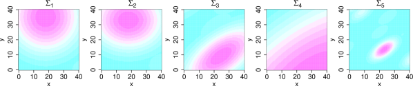
Figure 1: A Gaussian extreme value process realisation for ${\hbox{\hbox to0.0pt{$\Sigma$\hss}\kern 0.25pt\hbox to0.0pt{$\Sigma$\hss}\kern 0.25pt$\Sigma$}}_{1},\ldots,{\hbox{\hbox to0.0pt{$\Sigma$\hss}\kern 0.25pt\hbox to0.0pt{$\Sigma$\hss}\kern 0.25pt$\Sigma$}}_{5}$. Max-stable process simulation routines are available in the RandomFields package in R (Schlather, 2002).

Composite MLE’s based on 500 spatial extreme data simulations ($K=50$ sites and $N=100$) with the Gaussian extreme value model. True values are in [brackets]. Standard errors obtained through Godambe estimates and sample standard deviation (in parantheses). ${\widehat{\sigma}}^{2}_{1~{}}$ / s.e. ${\widehat{\sigma}}^{2}_{2~{}}$ / s.e. ${\widehat{\sigma}}^{2}_{12}$ / s.e. ${\hbox{\hbox to0.0pt{$\Sigma$\hss}\kern 0.25pt\hbox to0.0pt{$\Sigma$\hss}\kern 0.25pt$\Sigma$}}_{1}$: 306 [300] / 40.6 (44.7) 306 [300] / 39.8 (41.5) 1 [0] / 27.9 (27.7) ${\hbox{\hbox to0.0pt{$\Sigma$\hss}\kern 0.25pt\hbox to0.0pt{$\Sigma$\hss}\kern 0.25pt$\Sigma$}}_{2}$: 204 [200] / 26.7 (28.5) 305 [300] / 39.6 (39.7) 1 [0] / 21.9 (21.2) ${\hbox{\hbox to0.0pt{$\Sigma$\hss}\kern 0.25pt\hbox to0.0pt{$\Sigma$\hss}\kern 0.25pt$\Sigma$}}_{3}$: 202 [200] / 25.1 (26.1) 300 [300] / 37.3 (37.9) 150 [150] / 25.5 (26.1) ${\hbox{\hbox to0.0pt{$\Sigma$\hss}\kern 0.25pt\hbox to0.0pt{$\Sigma$\hss}\kern 0.25pt$\Sigma$}}_{4}$: 2053 [2000] / 495.2 (300.1) 3065 [3000] / 664.8 (483.1) 1550 [1500] / 412.0 (322.4) ${\hbox{\hbox to0.0pt{$\Sigma$\hss}\kern 0.25pt\hbox to0.0pt{$\Sigma$\hss}\kern 0.25pt$\Sigma$}}_{5}$: 20 [20] / 1.5 (1.6) 30 [30] / 2.3 (2.3) 15 [15] / 1.6 (1.6)

Table 4 summarizes estimator performance based on moderately sized datasets: $K=50$ sites and $N=100$ observations. Estimate means and standard errors over 500 data replications are reported, indicating good correspondence to the true values. There is no evidence of bias, even in cases where poorer performance may be expected such as very strong or weak dependence. Overall, the Godambe standard errors and sample standard deviations are consistent, though there is some discrepancy in the case of strong dependence. Here, the eigenvalues of ${\hbox{\hbox to0.0pt{$\Sigma$\hss}\kern 0.25pt\hbox to0.0pt{$\Sigma$\hss}\kern 0.25pt$\Sigma$}}_{4}^{-1}$ are $5\pm\sqrt{10}/7500$ and so we are near the parameter space boundary. Consequently, for some of the 500 replications, the asymptotic normality of ${{\widehat{\hbox{\hbox to0.0pt{$\psi$\hss}\kern 0.25pt\hbox to0.0pt{$\psi$\hss}\kern 0.25pt$\psi$}}}_{\text{\footnotesize{MCLE}}}}$ fails, and so the Godambe standard errors are not relevant.

Normalised mean squared error of extremal coefficient estimates based on 500 data simulations with $K=50$ sites and $N=100$ observations. Estimators are the composite MLE and those proposed by Smith (1990) and Schlather and Tawn (2003). Standard deviations are reported in parantheses. The values’ order of magnitude is $10^{-4}$. Composite MLE Smith Schlather & Tawn ${\hbox{\hbox to0.0pt{$\Sigma$\hss}\kern 0.25pt\hbox to0.0pt{$\Sigma$\hss}\kern 0.25pt$\Sigma$}}_{1}$: 3.1 ( 5.4) 18.4 (26.7) 17.3 (29.9) ${\hbox{\hbox to0.0pt{$\Sigma$\hss}\kern 0.25pt\hbox to0.0pt{$\Sigma$\hss}\kern 0.25pt$\Sigma$}}_{2}$: 2.9 ( 4.8) 19.1 (30.3) 18.9 (28.6) ${\hbox{\hbox to0.0pt{$\Sigma$\hss}\kern 0.25pt\hbox to0.0pt{$\Sigma$\hss}\kern 0.25pt$\Sigma$}}_{3}$: 2.5 ( 4.7) 21.9 (35.7) 21.1 (32.4) ${\hbox{\hbox to0.0pt{$\Sigma$\hss}\kern 0.25pt\hbox to0.0pt{$\Sigma$\hss}\kern 0.25pt$\Sigma$}}_{4}$: 3.0 (35.6) 10.9 (18.9)  6.7 (13.3) ${\hbox{\hbox to0.0pt{$\Sigma$\hss}\kern 0.25pt\hbox to0.0pt{$\Sigma$\hss}\kern 0.25pt$\Sigma$}}_{5}$: 0.3 ( 0.8) 30.3 (44.6) 25.5 (40.7)

Table 4 depicts normalised mean squared errors for three different estimators of the extremal coefficient functions: the composite MLE derived from the Gaussian extreme value model, and those proposed by Smith, (1990) and Schlather and Tawn, (2003). Normalized mean square errors are used to prevent the largest extremal coefficients from dominating. From Table 4, in general it is clear that the composite likelihood estimator is the most accurate. The standard deviation in the strong dependence case again suffers from the failure of the asymptotic normality of ${{\widehat{\hbox{\hbox to0.0pt{$\psi$\hss}\kern 0.25pt\hbox to0.0pt{$\psi$\hss}\kern 0.25pt$\psi$}}}_{\text{\footnotesize{MCLE}}}}$.

Composite MLEs for a varying number of sites ($K$) and observations ($N$), based on 500 simulations of spatial extreme data using the Gaussian extreme value model with covariance ${\hbox{\hbox to0.0pt{$\Sigma$\hss}\kern 0.25pt\hbox to0.0pt{$\Sigma$\hss}\kern 0.25pt$\Sigma$}}_{3}$ (Table 4). Standard deviations are reported in parantheses. $K$ $N=10$ $N=50$ $N=100$ $N=500$ True ${\widehat{\sigma}}^{2}_{1~{}}$ 10 245 (120.2) 207 (43.8) 205 (31.7) 199 (13.3) 200 50 244 ( 90.4) 208 (37.5) 200 (28.3) 199 (11.4) 100 239 ( 94.3) 205 (37.8) 202 (30.4) 199 (11.5) ${\widehat{\sigma}}^{2}_{2~{}}$ 10 353 (159.1) 305 (63.9) 301 (44.8) 298 (19.5) 300 50 353 (131.6) 309 (56.6) 303 (44.3) 298 (16.9) 100 361 (143.4) 307 (59.5) 301 (44.8) 299 (16.7) ${\widehat{\sigma}}_{12}$ 10 174 (108.9) 153 (41.8) 151 (31.9) 149 (13.4) 150 50 179 ( 91.2) 156 (38.8) 149 (28.6) 149 (11.4) 100 181 (100.9) 154 (39.2) 150 (29.7) 150 (11.2)

Estimator performance for a range of dataset sizes ($N=10,50,100,500$) and site numbers ($K=10,50,100$) is listed in Table 4, under 500 data replications of spatial dependence model ${\hbox{\hbox to0.0pt{$\Sigma$\hss}\kern 0.25pt\hbox to0.0pt{$\Sigma$\hss}\kern 0.25pt$\Sigma$}}_{3}$. As expected, the simulations indicate that there is some bias and larger variance for small $N$, and negligible bias and small variance for large $N$. Observe that, for fixed sample size, the number of sites does not impact the estimation results.

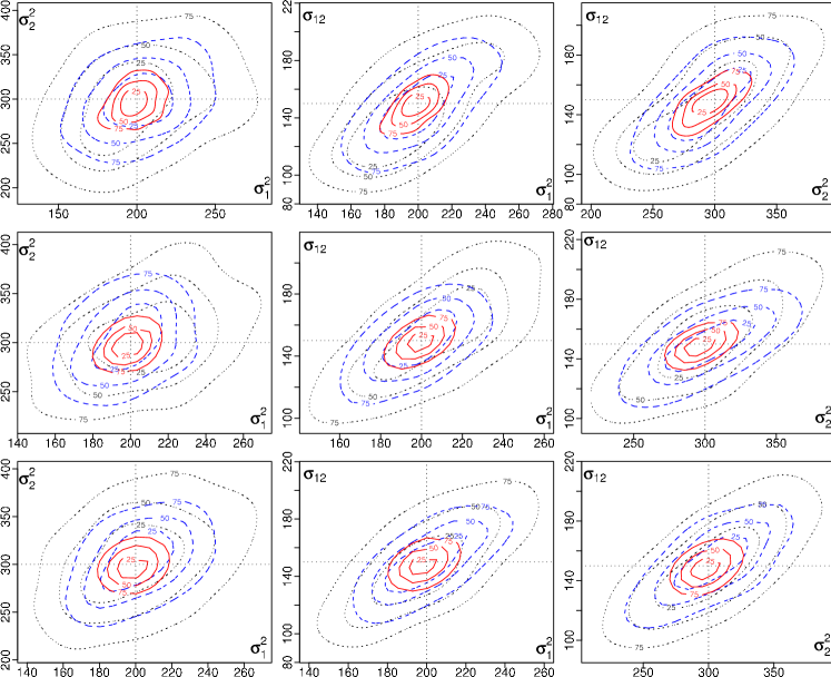
Figure 2: Composite MLE distribution estimates for $N=50$ (dotted line), $N=100$ (broken line) and $N=1000$ (solid line) observations over $K=10$ (top row), $K=50$ (centre row) and $K=100$ (bottom row) sites. Contours correspond to 0.25, 0.5 and 0.75 percentiles.

This behavior is illustrated in Figure 2, highlighting, in particular, good estimator performance with increasing $N$.

Finally, we consider model selection under misspecification. Figure 3 illustrates power curves (likelihood ratio tests) and rejection rates (CLIC) for two hypotheses, each versus their complement. Namely, $H_{0}:\sigma_{1}^{2}=200$ fixing $\sigma_{2}^{2}=300$ and $\sigma_{12}=150$ (top plots), and $H_{0}:\sigma_{1}^{2}=\sigma_{2}^{2}=200$ fixing $\sigma_{12}=0$ (bottom plots). All resulting curves are near-quadratic and, for the pairwise likelihood ratio based tests, rejection rates are close to the confidence level $\alpha=0.05$ when the null hypothesis is true. In this study, contrary to the results derived by Chandler and Bate, (2007), the adjustment of the $W$ statistic (8) Rotnitzky and Jewell, (1990) appears to have slightly more power – even when testing mutiple parameters. In contrast the CLIC statistic demonstrates poor performance, with the rejection rate under the true model reaching only $20\%$.

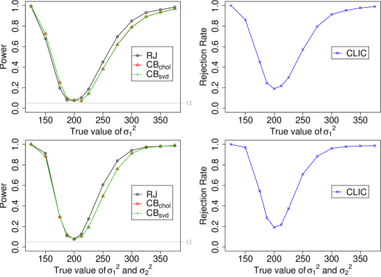
Figure 3: Left panels: Power curves for the composite likelihood ratio tests; $RJ$ (Rotnitzki and Jewell, 1990), and $CB_{chol}$ and $CB_{svd}$ (Chandler and Bate, 2007) using Cholesky and singular value decompositions. Right panels: CLIC rejection rates. Test levels are $\alpha=0.05$. Point estimates are based on 1000 data replications.

5 Application to U.S. precipitation data

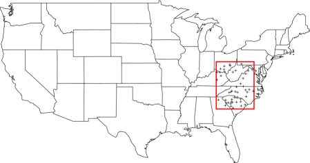
Figure 4: Locations of the $46$ gauging stations.

We illustrate the developed methodology in an analysis of U.S. precipitation data. These data consist of $46$ gauging stations with daily rainfall records over a period of $91$ years (Figure 4). We express the model GEV parameters as simple linear functions of longitude, lattitude and altitude. Further model variations, including additional environmental covariates, and regressions of the covariance $\Sigma$$\Sigma$$\Sigma$ on these covariates to examine spatial variations in extremal dependence were not considered.

Exploratory analyses of the functional complexity of the GEV parameters was performed by fitting independent GEV models to the data from each station and evaluating appropriate surface responses using standard techniques (e.g. ANOVA, Fisher tests). After identifying an upper limit to model complexity, we perform model selection on the pairwise composite likelihood of the Gaussian extreme value process using the methodologies outlined in Section 3.3.

Table 1: Some Gaussian extreme value processes and their corresponding maximised negative composite log-likelihood, degrees of freedom and the CLIC score.

Model		$-{\ell_{\mathcal{P}}}({{\widehat{\hbox{\hbox to0.0pt{$\psi$\hss}\kern 0.25pt\hbox to0.0pt{$\psi$\hss}\kern 0.25pt$\psi$}}}_{\text{\footnotesize{MCLE}}}};{\bf y})$	d.f.	CLIC
$M_{0}:$	$\mu(x)=\alpha_{0}+\alpha_{1}(\mbox{lat})+\alpha_{2}(\mbox{alt})+\alpha_{3}(\mbox{lon})$	412,110.2	12	12,848,229
	$\sigma(x)=\beta_{0}+\beta_{1}(\mbox{lat})+\beta_{2}(\mbox{alt})+\beta_{2}(\mbox{lon})$
	$\xi(x)=\gamma_{0}$
$M_{1}:$	$\mu(x)=\alpha_{0}+\alpha_{1}(\mbox{lat})+\alpha_{2}(\mbox{alt})$	412,110.9	11	16,096,068
	$\sigma(x)=\beta_{0}+\beta_{1}(\mbox{lat})+\beta_{2}(\mbox{alt})+\beta_{3}(\mbox{lon})$
	$\xi(x)=\gamma_{0}$
$M_{2}:$	$\mu(x)=\alpha_{0}+\alpha_{1}(\mbox{lat})+\alpha_{2}(\mbox{alt})+\alpha_{3}(\mbox{lon})$	412,113.3	11	1,008,997
	$\sigma(x)=\beta_{0}+\beta_{1}(\mbox{lat})+\beta_{2}(\mbox{alt})$
	$\xi(x)=\gamma_{0}$
$M_{3}:$	$\mu(x)=\alpha_{0}+\alpha_{1}(\mbox{lat})+\alpha_{3}(\mbox{lon})$	412,234.1	11	1,926,389,242
	$\sigma(x)=\beta_{0}+\beta_{1}(\mbox{lat})+\beta_{2}(\mbox{alt})+\beta_{3}(\mbox{lon})$
	$\xi(x)=\gamma_{0}$
$M_{4}:$	$\mu(x)=\alpha_{0}+\alpha_{1}(\mbox{lat})+\alpha_{2}(\mbox{alt})+\alpha_{3}(\mbox{lon})$	412,380.5	11	33,209,042
	$\sigma(x)=\beta_{0}+\beta_{1}(\mbox{lat})+\beta_{3}(\mbox{lon})$
	$\xi(x)=\gamma_{0}$
$\mathbf{M_{5}:}$	$\mathbf{\mu(x)=\alpha_{0}+\alpha_{1}(\mbox{lat})+\alpha_{2}(\mbox{alt})}$	412,113.3	10	1,008,261
	$\mathbf{\mathbf{\sigma(x)=\beta_{0}+\beta_{1}(\mbox{lat})+\beta_{2}(\mbox{alt})}}$
	$\mathbf{\xi(x)=\gamma_{0}}$
$M_{6}:$	$\mu(x)=\alpha_{0}+\alpha_{1}(\mbox{lat})$	412,237.3	9	1,086,347
	$\sigma(x)=\beta_{0}+\beta_{1}(\mbox{lat})+\beta_{2}(\mbox{alt})$
	$\xi(x)=\gamma_{0}$

Table 1 summarizes some of the different models investigated. According to the CLIC criterion, model $M_{5}$ (in bold) is the preferred choice, although models $M_{2}$ and $M_{6}$ also appear competitive. Despite the relatively poor performance of the CLIC criterion for model selection (see Section 4), the same conclusions are obtained from the deviance based tests, with $p$-values around 0.9. For model $M_{5}$, the covariance $\Sigma$$\Sigma$$\Sigma$ is estimated as $\sigma_{1}^{2}=0.06323$ $(0.06463)$, $\sigma_{12}=0.01334$ $(0.03661)$ and $\sigma_{2}^{2}=0.02581$ $(0.02538)$, where the parantheses indicate standard errors.

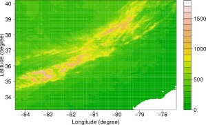
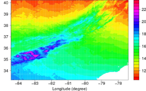
Figure 5: Left: Elevation map (metres) of the region; Right: Pointwise 50-year return level map (cm) estimated from the fitted Gaussian extreme value process.

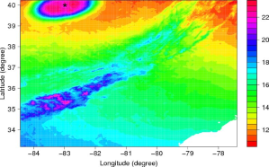
Figure 6: Left: Contour plot of the extremal coefficient; Right: Pointwise 50-year, conditional return level map (cm) estimated from the fitted Gaussian extreme value process. The star indicates the fixed site used in the computation of the conditional return levels.

Figure 5 (right plot) illustrates the spatial variation of pointwise 50-year return level estimates. Comparison to the regional elevation map (left plot) indicates that the most extreme precipitation events occur in mountainous regions. Figure 6 (left plot) also depicts the strength of spatial dependence through the extremal coefficient function. There is clear evidence of anisotropy, with stronger dependence in the north-east/south-west direction. Interestingly, this axis corresponds to the shape of the Appalachian Mountains as well as the coastline. Accordingly, this directional extremal dependence may be the consequence of storms following either the coastline or the massif. Finally, conditioning of a fixed site (and for a given threshold) by using the pairwise conditional distribution, the conditional $q$-year return level estimates can easily be provided. Figure 6 (right plot) illustrates the spatial variation of conditional pointwise 50-year return level estimates, given the fixed site indicated by the star.

6 Conclusion

As a natural generalisation of extremal dependence structures, max-stable processes are a powerful tool for the modelling of multivariate extremes. Unfortunately, the intractability of the multivariate density function precludes inference except in trivial cases (e.g. bivariate), or requires additional approximations and immense computational overheads (Jiang and Turnbull,, 2004; Sisson et al.,, 2007; Peters et al.,, 2008).

This article has developed composite likelihood-based inferential methods for general max-stable processes. Our results demonstrate good applicability in the spatial context. The benefits of this likelihood-based approach are the flexible joint modelling of marginal and dependence parameters, coupled with good estimator behaviour with finite samples, all at moderate computational cost.

Modifications of the model formulation would draw alternative representations of extremal modelling into the composite-likelihood based framework, given the known links between these and block maxima (GEV) approaches (e.g. Coles, (2001)). These include threshold excess models for marginals (Davison and Smith, 1990), and the limiting Poisson characterisation of extremes. The obvious practical benefit from these extensions would be the incorporation of more data into the modelling process.

Appendix

We present explicit expressions for the distribution function (3), density function (4) and the derivatives required for the estimated covariance matrix in Section 3.2

A.1: Vector notation

Let $f$ be a real-valued function in the $d\times 1$ vector ${\bf x}=(x_{1},\ldots,x_{d})$. Then the $1\times d$ derivative vector, ${\sf D}_{{\bf x}}f({\bf x})$, has $i$-th element $\partial f({\bf x})/\partial x_{i}$. The corresponding Hessian matrix is given by ${\sf H}_{{\bf x}}f({\bf x})={\sf D}_{{\bf x}}\{{\sf D}_{{\bf x}}f({\bf x})\}^{\top}$.

If ${\bf a}=(a_{1},\ldots,a_{d})$ and ${\bf b}=(b_{1},\ldots,b_{d})$ are two $d\times 1$ vectors, then element-wise multiplication is denoted by ${\bf a}\odot{\bf b}=(a_{1}b_{1},\ldots,a_{d}b_{d})$. The expression ${\bf a}/{\bf b}$ denotes element-wise division $(a_{1}/b_{1},\ldots,a_{d}/b_{d})$. Scalar functions applied to vectors are also evaluated element-wise. For example, ${\bf a}^{-1/\xi}=(a_{1}^{-1/\xi},\ldots,a_{d}^{-1/\xi})$.

A.2: Derivation of the bivariate distribution function

In order to derive the cumulative distribution function (3), considering formula (2) and the assumptions of Section 2.3, we need to solve:

$$\begin{split}F(z_{i},z_{j})&=\exp\left\{-\int_{-\infty}^{\infty}\int_{-\infty}^{\infty}\max\left(\frac{f(x_{1},x_{2})}{z_{i}},\frac{f(x_{1}-t_{1},x_{2}-t_{2})}{z_{j}}\right)\,\mbox{d}x_{1}\,\mbox{d}x_{2}\right\}\\ &=\exp\Bigg{\{}-\int_{-\infty}^{\infty}\int_{-\infty}^{\infty}\frac{f(x_{1},x_{2})}{z_{i}}\mathbb{I}\left(\frac{f(x_{1},x_{2})}{z_{i}}\geq\frac{f(x_{1}-t_{1},x_{2}-t_{2})}{z_{j}}\right)\,\mbox{d}x_{1}\,\mbox{d}x_{2}\\ &-\int_{-\infty}^{\infty}\int_{-\infty}^{\infty}\frac{f(x_{1}-t_{1},x_{2}-t_{2})}{z_{j}}\mathbb{I}\left(\frac{f(x_{1}-t_{1},x_{2}-t_{2})}{z_{j}}\geq\frac{f(x_{1},x_{2})}{z_{i}}\right)\,\mbox{d}x_{1}\,\mbox{d}x_{2}\Bigg{\}},\end{split}$$

where $f(x_{1},x_{2})$ is the bivariate normal density of $(X_{1},X_{2})\sim N((0,0)^{\top},{\hbox{\hbox to0.0pt{$\Sigma$\hss}\kern 0.25pt\hbox to0.0pt{$\Sigma$\hss}\kern 0.25pt$\Sigma$}})$, and for brevity we set ${\bf h}=({\bf t}_{j}-{\bf t}_{i})^{\top}\equiv(t_{1},t_{2})^{\top}$. Recall from (3) that

$$a({\bf h})=({\bf h}^{T}{\hbox{\hbox to0.0pt{$\Sigma$\hss}\kern 0.25pt\hbox to0.0pt{$\Sigma$\hss}\kern 0.25pt$\Sigma$}}^{-1}{\bf h})^{1/2}=\frac{1}{\sqrt{(1-\rho^{2})}}\left(\frac{t_{1}^{2}}{\sigma_{1}^{2}}-\frac{2\rho t_{1}t_{2}}{\sigma_{1}\sigma_{2}}+\frac{t_{2}^{2}}{\sigma_{2}^{2}}\right)^{1/2}$$

where $\rho=\sigma_{12}/\sigma_{1}\sigma_{2}$. Consider first the case $(t_{1}\sigma_{2}-\rho t_{2}\sigma_{1})>0$. Note that $f(x_{1},x_{2})/z_{i}\geq f(x_{1}-t_{1},x_{2}-t_{2})/z_{j}$ implies that

$$\begin{split}&\exp\left\{-\frac{1}{2(1-\rho^{2})}\left(\frac{x_{1}^{2}}{\sigma_{1}^{2}}-\frac{2\rho x_{1}x_{2}}{\sigma_{1}\sigma_{2}}+\frac{x_{2}^{2}}{\sigma_{2}^{2}}\right)\right\}/z_{i}\\ &\geq\exp\left\{-\frac{1}{2(1-\rho^{2})}\left(\frac{(x_{1}-t_{1})^{2}}{\sigma_{1}^{2}}-\frac{2\rho(x_{1}-t_{1})(x_{2}-t_{2})}{\sigma_{1}\sigma_{2}}+\frac{(x_{2}-t_{2})^{2}}{\sigma_{2}^{2}}\right)\right\}/z_{i}\\ &\Leftrightarrow x_{1}\leq\frac{\sigma_{1}^{2}\sigma_{2}}{2(t_{1}\sigma_{2}-\rho t_{2}\sigma_{1})}\left(\frac{t_{1}^{2}}{\sigma_{1}^{2}}-\frac{2\rho t_{1}t_{2}}{\sigma_{1}\sigma_{2}}+\frac{t_{2}^{2}}{\sigma_{2}^{2}}\right)+\frac{\sigma_{1}^{2}\sigma_{2}(1-\rho^{2})}{t_{1}\sigma_{2}-\rho t_{2}\sigma_{1}}\log\frac{z_{j}}{z_{i}}-\frac{x_{2}(t_{2}\sigma_{1}^{2}-\rho t_{1}\sigma_{1}\sigma_{2})}{t_{1}\sigma_{2}-\rho t_{2}\sigma_{1}}\\ &\Leftrightarrow x_{1}\leq c.\end{split}$$

From this, it follows that

$$\begin{split}&\int_{-\infty}^{\infty}\int_{-\infty}^{\infty}\frac{f(x_{1},x_{2})}{z_{i}}\mathbb{I}\left(\frac{f(x_{1},x_{2})}{z_{i}}\geq\frac{f(x_{1}-t_{1},x_{2}-t_{2})}{z_{j}}\right)\,\mbox{d}x_{1}\,\mbox{d}x_{2}\\ &=\frac{1}{z_{i}}\int_{-\infty}^{\infty}\int_{-\infty}^{c}\frac{1}{2\pi\sqrt{1-\rho^{2}}}\exp\left\{-\frac{1}{2(1-\rho^{2})}\left(\frac{x_{1}^{2}}{\sigma_{1}^{2}}-\frac{2\rho x_{1}x_{2}}{\sigma_{1}\sigma_{2}}+\frac{x_{2}^{2}}{\sigma_{2}^{2}}\right)\right\}\,\mbox{d}x_{1}\,\mbox{d}x_{2}\\ &=\frac{1}{z_{i}}\int_{-\infty}^{\infty}\varphi(x_{2})\int_{-\infty}^{c}\varphi\left(\frac{x_{1}-\rho\sigma_{1}x_{2}/\sigma_{2}}{\sigma_{1}\sqrt{1-\rho^{2}}}\right)\,\mbox{d}x_{1}\,\mbox{d}x_{2}\\ &=\frac{1}{z_{i}}\int_{-\infty}^{\infty}\varphi(x_{2})\Phi\left(\frac{c-\rho\sigma_{1}x_{2}/\sigma_{2}}{\sigma_{1}\sqrt{1-\rho^{2}}}\right)\mbox{d}x_{2}\\ &=\frac{1}{z_{i}}\Phi\left(\frac{1}{2\sqrt{(1-\rho^{2})}}\left(\frac{t_{1}^{2}}{\sigma_{1}^{2}}-\frac{2\rho t_{1}t_{2}}{\sigma_{1}\sigma_{2}}+\frac{t_{2}^{2}}{\sigma_{2}^{2}}\right)^{1/2}+\left(\frac{t_{1}^{2}}{\sigma_{1}^{2}}-\frac{2\rho t_{1}t_{2}}{\sigma_{1}\sigma_{2}}+\frac{t_{2}^{2}}{\sigma_{2}^{2}}\right)^{-1/2}\frac{\log z_{j}/z_{i}}{(1-\rho^{2})^{-1/2}}\right)\\ &=\frac{1}{z_{i}}\Phi\left(\frac{a({\bf h})}{2}+\frac{\log z_{j}/z_{i}}{a({\bf h})}\right).\end{split}$$

Similarly,

$$\frac{f(x_{1}-t_{1},x_{2}-t_{2})}{z_{j}}\geq\frac{f(x_{1},x_{2})}{z_{i}}\Leftrightarrow x_{1}\geq c.$$

It then follows that

$$\begin{split}&\int_{-\infty}^{\infty}\int_{-\infty}^{\infty}\frac{f(x_{1}-t_{1},x_{2}-t_{2})}{z_{j}}\mathbb{I}\left(\frac{f(x_{1},x_{2})}{z_{i}}\geq\frac{f(x_{1}-t_{1},x_{2}-t_{2})}{z_{j}}\right)\,\mbox{d}x_{1}\,\mbox{d}x_{2}\\ &=\frac{1}{z_{j}}\int_{-\infty}^{\infty}\int_{c}^{\infty}\frac{1}{2\pi\sqrt{1-\rho^{2}}}\exp\left\{-\frac{1}{2(1-\rho^{2})}\left(\frac{(x_{1}-t_{1})^{2}}{\sigma_{1}^{2}}-\frac{2\rho(x_{1}-t_{1})(x_{2}-t_{2})}{\sigma_{1}\sigma_{2}}+\frac{(x_{2}-t_{2})^{2}}{\sigma_{2}^{2}}\right)\right\}\,\mbox{d}x_{1}\,\mbox{d}x_{2}\\ &=\frac{1}{z_{j}}\int_{-\infty}^{\infty}\varphi(x_{2}-t_{2})\int_{c}^{\infty}\varphi\left(\frac{(x_{1}-t_{1})-\rho\sigma_{1}(x_{2}-t_{2})/\sigma_{2}}{\sigma_{1}\sqrt{1-\rho^{2}}}\right)\,\mbox{d}x_{1}\,\mbox{d}x_{2}\\ &=\frac{1}{z_{j}}\int_{-\infty}^{\infty}\varphi(x_{2}-t_{2})\left\{1-\Phi\left(\frac{c-\rho\sigma_{1}(x_{2}-t_{2})/\sigma_{2}}{\sigma_{1}\sqrt{1-\rho^{2}}}\right)\right\}\mbox{d}x_{2}\\ &=\frac{1}{z_{j}}\Phi\left(\frac{1}{2\sqrt{(1-\rho^{2})}}\left(\frac{t_{1}^{2}}{\sigma_{1}^{2}}-\frac{2\rho t_{1}t_{2}}{\sigma_{1}\sigma_{2}}+\frac{t_{2}^{2}}{\sigma_{2}^{2}}\right)^{1/2}+\left(\frac{t_{1}^{2}}{\sigma_{1}^{2}}-\frac{2\rho t_{1}t_{2}}{\sigma_{1}\sigma_{2}}+\frac{t_{2}^{2}}{\sigma_{2}^{2}}\right)^{-1/2}\frac{\log z_{i}/z_{j}}{(1-\rho^{2})^{-1/2}}\right)\\ &=\frac{1}{z_{j}}\Phi\left(\frac{a({\bf h})}{2}+\frac{\log z_{i}/z_{j}}{a({\bf h})}\right),\end{split}$$

and the form of the distribution (3) is confirmed. Observe, that the same result is obtained for the case $(t_{1}\sigma_{2}-\rho t_{2}\sigma_{1})<0$. See also Smith, (1990) and De Haan and Pereira, (2006).

A.3: Derivation of the bivariate density function

In order to derive the bivariate density function (4) we require the second-order derivative of

$$F(z_{i},z_{j})=\exp\left(-\frac{\Phi(w)}{z_{i}}-\frac{\Phi(v)}{z_{j}}\right)$$

with respect to $z_{i}$ and $z_{j}$, where for brevity we set $a\equiv a(h)$, $w\equiv w(h)$ and $v\equiv v(h)$ and write $w=a/2+\log(z_{j}/z_{i})/a$ and $v=a-w$. The differentiation gives

$$\begin{split}&f(z_{i},z_{j})\equiv\frac{\partial^{2}}{\partial z_{i}\partial z_{j}}F(z_{i},z_{j})=\\ &\exp\left(-\frac{\Phi(w)}{z_{i}}-\frac{\Phi(v)}{z_{j}}\right)\Bigg{\{}\frac{\partial}{\partial z_{i}}\left(-\frac{\Phi(w)}{z_{i}}-\frac{\Phi(v)}{z_{j}}\right)\frac{\partial}{\partial z_{j}}\left(-\frac{\Phi(w)}{z_{i}}-\frac{\Phi(v)}{z_{j}}\right)+\frac{\partial^{2}}{\partial z_{i}\partial z_{j}}\left(-\frac{\Phi(w)}{z_{i}}-\frac{\Phi(v)}{z_{j}}\right)\Bigg{\}}.\end{split}$$

First-order differentation gives

$$\frac{\partial}{\partial z_{i}}\left(-\frac{\Phi(w)}{z_{i}}-\frac{\Phi(v)}{z_{j}}\right)=\frac{\Phi(w)}{z_{i}^{2}}+\frac{\varphi(w)}{az_{i}^{2}}-\frac{\varphi(v)}{az_{i}z_{j}},\quad\frac{\partial}{\partial z_{j}}\left(-\frac{\Phi(w)}{z_{i}}-\frac{\Phi(v)}{z_{j}}\right)=\frac{\Phi(v)}{z_{j}^{2}}+\frac{\varphi(v)}{az_{j}^{2}}-\frac{\varphi(w)}{az_{i}z_{j}},$$

using the results

$$\frac{\partial\Phi(w)}{\partial z_{i}}=-\frac{\varphi(w)}{az_{i}},\quad\frac{\partial\Phi(v)}{\partial z_{i}}=\frac{\varphi(v)}{az_{i}}\quad\mbox{and}\quad\frac{\partial w}{\partial z_{i}}=-\frac{1}{az_{i}},\quad\frac{\partial v}{\partial z_{i}}=\frac{1}{az_{i}}.$$

Second-order differentation yields

$$\frac{\partial^{2}}{\partial z_{i}\partial z_{j}}\left(-\frac{\Phi(w)}{z_{i}}-\frac{\Phi(v)}{z_{j}}\right)=\frac{v\,\varphi(w)}{a^{2}z_{i}^{2}z_{j}}+\frac{w\,\varphi(v)}{a^{2}z_{i}z_{j}^{2}},$$

using

$$\frac{\partial\varphi(w)}{\partial z_{i}}=\frac{w\varphi(w)}{az_{i}}\quad\mbox{and}\quad\frac{\partial\varphi(v)}{\partial z_{i}}=-\frac{v\varphi(v)}{az_{i}}.$$

Substituting, we obtain the probability density function

$$\begin{split}f(z_{i},z_{j})&=\exp\bigg{\{}-\frac{\Phi(w)}{z_{i}}-\frac{\Phi(v)}{z_{j}}\bigg{\}}\Bigg{\{}\left(\frac{\Phi(w)}{z_{i}^{2}}+\frac{\varphi(w)}{az_{i}^{2}}-\frac{\varphi(v)}{az_{i}z_{j}}\right)\\ &\bigg{(}\frac{\Phi(v)}{z_{j}^{2}}+\frac{\varphi(v)}{az_{j}^{2}}-\frac{\varphi(w)}{az_{i}z_{j}}\bigg{)}+\bigg{(}\frac{v\,\varphi(w)}{a^{2}z_{i}^{2}z_{j}}+\frac{w\,\varphi(v)}{a^{2}z_{i}z_{j}^{2}}\bigg{)}\Bigg{\}}.\end{split}$$

A.4: An expression for the squared score statistic

From Section 3.2 the term $\text{J}({\hbox{\hbox to0.0pt{$\psi$\hss}\kern 0.25pt\hbox to0.0pt{$\psi$\hss}\kern 0.25pt$\psi$}})$ of the Godambe information matrix can be estimated from

$$\sum_{i=1}^{\mathcal{K}}\sum_{j=i+1}^{\mathcal{K}-1}{{\sf D}_{{\text{\footnotesize{\hbox{\hbox to0.0pt{$\psi$\hss}\kern 0.25pt\hbox to0.0pt{$\psi$\hss}\kern 0.25pt$\psi$}}}}}}\log f({\bf y}_{i},{\bf y}_{j};{\hbox{\hbox to0.0pt{$\psi$\hss}\kern 0.25pt\hbox to0.0pt{$\psi$\hss}\kern 0.25pt$\psi$}})^{\top}\,{{\sf D}_{{\text{\footnotesize{\hbox{\hbox to0.0pt{$\psi$\hss}\kern 0.25pt\hbox to0.0pt{$\psi$\hss}\kern 0.25pt$\psi$}}}}}}\log f({\bf y}_{i},{\bf y}_{j};{\hbox{\hbox to0.0pt{$\psi$\hss}\kern 0.25pt\hbox to0.0pt{$\psi$\hss}\kern 0.25pt$\psi$}}),$$

where ${\hbox{\hbox to0.0pt{$\psi$\hss}\kern 0.25pt\hbox to0.0pt{$\psi$\hss}\kern 0.25pt$\psi$}}^{\top}=({\hbox{\hbox to0.0pt{$\sigma$\hss}\kern 0.25pt\hbox to0.0pt{$\sigma$\hss}\kern 0.25pt$\sigma$}},{\hbox{\hbox to0.0pt{$\beta$\hss}\kern 0.25pt\hbox to0.0pt{$\beta$\hss}\kern 0.25pt$\beta$}}_{\mu},{\hbox{\hbox to0.0pt{$\beta$\hss}\kern 0.25pt\hbox to0.0pt{$\beta$\hss}\kern 0.25pt$\beta$}}_{\lambda},{\hbox{\hbox to0.0pt{$\beta$\hss}\kern 0.25pt\hbox to0.0pt{$\beta$\hss}\kern 0.25pt$\beta$}}_{\xi})$, ${\hbox{\hbox to0.0pt{$\sigma$\hss}\kern 0.25pt\hbox to0.0pt{$\sigma$\hss}\kern 0.25pt$\sigma$}}^{\top}=({\hbox{\hbox to0.0pt{$\sigma$\hss}\kern 0.25pt\hbox to0.0pt{$\sigma$\hss}\kern 0.25pt$\sigma$}}_{11}^{2},{\hbox{\hbox to0.0pt{$\sigma$\hss}\kern 0.25pt\hbox to0.0pt{$\sigma$\hss}\kern 0.25pt$\sigma$}}_{12},{\hbox{\hbox to0.0pt{$\sigma$\hss}\kern 0.25pt\hbox to0.0pt{$\sigma$\hss}\kern 0.25pt$\sigma$}}_{22}^{2})$ and where each parameter $\beta$$\beta$$\beta$ is $p$-dimensional vector of coefficients. The bivariate log-density has the form

$$\log f({\bf y}_{i},{\bf y}_{j};{\hbox{\hbox to0.0pt{$\psi$\hss}\kern 0.25pt\hbox to0.0pt{$\psi$\hss}\kern 0.25pt$\psi$}})=\text{A}+\log(\text{B}\odot\text{C}+\text{D})+\text{E},$$

where

$$\text{A}=-\frac{\Phi({\bf w})}{{\bf z}_{i}}-\frac{\Phi({\bf v})}{{\bf z}_{j}},\qquad\text{B}=\frac{\Phi({\bf w})}{{\bf z}_{i}^{2}}+\frac{\varphi({\bf w})}{{\bf a}\odot{\bf z}_{i}^{2}}-\frac{\varphi({\bf v})}{{\bf a}\odot{\bf z}_{i}\odot{\bf z}_{j}},\,$$

$$\text{C}=\frac{\Phi({\bf v})}{{\bf z}_{j}^{2}}+\frac{\varphi({\bf v})}{{\bf a}\odot{\bf z}_{j}^{2}}-\frac{\varphi({\bf w})}{{\bf a}\odot{\bf z}_{i}\odot{\bf z}_{j}},\qquad\text{D}=\frac{{\bf v}\odot\varphi({\bf w})}{{\bf a}^{2}\odot{\bf z}_{i}^{2}\odot{\bf z}_{j}}+\frac{{\bf w}\odot\varphi({\bf v})}{{\bf a}^{2}\odot{\bf z}_{i}\odot{\bf z}_{j}^{2}}\,$$

$$\mbox{and}\quad\text{E}=\log\left\{\frac{1}{\lambda_{i}\lambda_{j}}\left({\bf 1}+\xi_{i}\frac{{\bf y}_{i}-\mu_{i}{\bf 1}}{\lambda_{i}}\right)_{+}^{\frac{1}{\xi_{i}}-1}\left({\bf 1}+\xi_{j}\frac{{\bf y}_{j}-\mu_{j}{\bf 1}}{\lambda_{j}}\right)_{+}^{\frac{1}{\xi_{j}}-1}\right\}$$

and where ${\bf 1}^{\top}=(1,\ldots,1)$, $\mu_{i}=({\bf X}_{{\text{\footnotesize{\hbox{\hbox to0.0pt{$\beta$\hss}\kern 0.25pt\hbox to0.0pt{$\beta$\hss}\kern 0.25pt$\beta$}}}}_{\mu}}{\hbox{\hbox to0.0pt{$\beta$\hss}\kern 0.25pt\hbox to0.0pt{$\beta$\hss}\kern 0.25pt$\beta$}}_{\mu})_{i}$, $\xi_{i}=({\bf X}_{{\text{\footnotesize{\hbox{\hbox to0.0pt{$\beta$\hss}\kern 0.25pt\hbox to0.0pt{$\beta$\hss}\kern 0.25pt$\beta$}}}}_{\xi}}{\hbox{\hbox to0.0pt{$\beta$\hss}\kern 0.25pt\hbox to0.0pt{$\beta$\hss}\kern 0.25pt$\beta$}}_{\xi})_{i}$ and $\log(\psi_{i})=({\bf X}_{{\text{\footnotesize{\hbox{\hbox to0.0pt{$\beta$\hss}\kern 0.25pt\hbox to0.0pt{$\beta$\hss}\kern 0.25pt$\beta$}}}}_{\psi}}{\hbox{\hbox to0.0pt{$\beta$\hss}\kern 0.25pt\hbox to0.0pt{$\beta$\hss}\kern 0.25pt$\beta$}}_{\psi})_{i}$. The GEV parameters are related to the predictors by the form (7). We assume identity link functions for the location and shape parameters and exponential for the scale. The term E corresponds to the log of the determinat of the Jacobian matrix associated with the transformation (6), see Section 3.2.

The first-order derivative term of the square score statistic is defined by

$${\sf D}_{{\text{\footnotesize{\hbox{\hbox to0.0pt{$\psi$\hss}\kern 0.25pt\hbox to0.0pt{$\psi$\hss}\kern 0.25pt$\psi$}}}}}\log f({\bf y}_{i},{\bf y}_{j};{\hbox{\hbox to0.0pt{$\psi$\hss}\kern 0.25pt\hbox to0.0pt{$\psi$\hss}\kern 0.25pt$\psi$}})=({\sf D}_{{\hbox{\hbox to0.0pt{$\sigma$\hss}\kern 0.25pt\hbox to0.0pt{$\sigma$\hss}\kern 0.25pt$\sigma$}}}\log f({\hbox{\hbox to0.0pt{$\psi$\hss}\kern 0.25pt\hbox to0.0pt{$\psi$\hss}\kern 0.25pt$\psi$}}),{\sf D}_{{\text{\footnotesize{\hbox{\hbox to0.0pt{$\beta$\hss}\kern 0.25pt\hbox to0.0pt{$\beta$\hss}\kern 0.25pt$\beta$}}}}_{\mu}}\log f({\hbox{\hbox to0.0pt{$\psi$\hss}\kern 0.25pt\hbox to0.0pt{$\psi$\hss}\kern 0.25pt$\psi$}}),{\sf D}_{{\text{\footnotesize{\hbox{\hbox to0.0pt{$\beta$\hss}\kern 0.25pt\hbox to0.0pt{$\beta$\hss}\kern 0.25pt$\beta$}}}}_{\lambda}}\log f({\hbox{\hbox to0.0pt{$\psi$\hss}\kern 0.25pt\hbox to0.0pt{$\psi$\hss}\kern 0.25pt$\psi$}}),{\sf D}_{{\text{\footnotesize{\hbox{\hbox to0.0pt{$\beta$\hss}\kern 0.25pt\hbox to0.0pt{$\beta$\hss}\kern 0.25pt$\beta$}}}}_{\xi}}\log f({\hbox{\hbox to0.0pt{$\psi$\hss}\kern 0.25pt\hbox to0.0pt{$\psi$\hss}\kern 0.25pt$\psi$}}))$$

where for brevity we write $\log f({\hbox{\hbox to0.0pt{$\psi$\hss}\kern 0.25pt\hbox to0.0pt{$\psi$\hss}\kern 0.25pt$\psi$}})\equiv\log f({\bf y}_{i},{\bf y}_{j};{\hbox{\hbox to0.0pt{$\psi$\hss}\kern 0.25pt\hbox to0.0pt{$\psi$\hss}\kern 0.25pt$\psi$}})$. Vector differential calculus (e.g. Wand, (2002)) leads to

$$\begin{split}{\sf D}_{\sigma}\log f({\hbox{\hbox to0.0pt{$\psi$\hss}\kern 0.25pt\hbox to0.0pt{$\psi$\hss}\kern 0.25pt$\psi$}})&\equiv\Bigg{[}-\frac{{\bf v}\odot\varphi({\bf w})}{{\bf a}\odot{\bf z}_{i}}-\frac{{\bf w}\odot\varphi({\bf v})}{{\bf a}\odot{\bf z}_{j}}+\bigg{\{}\text{C}\odot\bigg{(}\frac{({\bf w}^{2}-{\bf 1})\odot\varphi({\bf v})}{{\bf a}^{2}\odot{\bf z}_{j}^{2}}+\frac{({\bf 1}+{\bf w}\odot{\bf v})\odot\varphi({\bf w})}{{\bf a}^{2}\odot{\bf z}_{i}\odot{\bf z}_{j}}\bigg{)}\\ &+\text{B}\odot\bigg{(}\frac{({\bf v}^{2}-{\bf 1})\odot\varphi({\bf w})}{{\bf a}^{2}\odot{\bf z}_{i}^{2}}+\frac{({\bf 1}+{\bf w}\odot{\bf v})\odot\varphi({\bf v})}{{\bf a}^{2}\odot{\bf z}_{i}\odot{\bf z}_{j}}\bigg{)}+\frac{({\bf w}-2{\bf v}-{\bf w}\odot{\bf v}^{2})\odot\varphi({\bf w})}{{\bf a}^{3}\odot{\bf z}_{i}^{2}\odot{\bf z}_{j}}\\ &+\frac{({\bf v}-2{\bf w}-{\bf v}\odot{\bf w}^{2})\odot\varphi({\bf v})}{{\bf a}^{3}\odot{\bf z}_{j}^{2}\odot{\bf z}_{i}}\bigg{\}}/(\text{B}\odot\text{C}+\text{D})\Bigg{]}{\bf s}^{\top},\end{split}$$

where ${\bf s}^{\top}\equiv(t_{1}^{2},\,2\,t_{1}\,t_{2},\,t_{2}^{2})$, using the results

$${\sf D}_{{\hbox{\hbox to0.0pt{$\sigma$\hss}\kern 0.25pt\hbox to0.0pt{$\sigma$\hss}\kern 0.25pt$\sigma$}}}{\bf w}=\frac{{\bf v}}{{\bf a}}\,{\bf s}^{\top},\qquad{\sf D}_{{\hbox{\hbox to0.0pt{$\sigma$\hss}\kern 0.25pt\hbox to0.0pt{$\sigma$\hss}\kern 0.25pt$\sigma$}}}\Phi({\bf w})=\frac{{\bf v}\odot\varphi({\bf w})}{{\bf a}}\,{\bf s}^{\top},\qquad{\sf D}_{{\hbox{\hbox to0.0pt{$\sigma$\hss}\kern 0.25pt\hbox to0.0pt{$\sigma$\hss}\kern 0.25pt$\sigma$}}}\varphi({\bf w})=-\frac{{\bf w}\odot{\bf v}\varphi({\bf w})}{{\bf a}}\,{\bf s}^{\top}$$

$$\mbox{and}\quad{\sf D}_{{\hbox{\hbox to0.0pt{$\sigma$\hss}\kern 0.25pt\hbox to0.0pt{$\sigma$\hss}\kern 0.25pt$\sigma$}}}{\bf v}\odot\varphi({\bf w})=\frac{{\bf w}\odot({\bf 1}-{\bf v}^{2})\varphi({\bf w})}{{\bf a}}\,{\bf s}^{\top}.$$

The first-order derivativies of ${\bf v}$, $\Phi({\bf v})$, $\varphi({\bf v})$ and ${\bf w}\odot\varphi({\bf v})$ are the same as the above, substituting ${\bf v}$ for ${\bf w}$. Similarly for the second term we have

$$\begin{split}{\sf D}_{{\text{\footnotesize{\hbox{\hbox to0.0pt{$\beta$\hss}\kern 0.25pt\hbox to0.0pt{$\beta$\hss}\kern 0.25pt$\beta$}}}}_{\mu}}\log f({\hbox{\hbox to0.0pt{$\psi$\hss}\kern 0.25pt\hbox to0.0pt{$\psi$\hss}\kern 0.25pt$\psi$}})&\equiv\Bigg{\{}\bigg{(}\frac{\varphi({\bf w})+{\bf a}\odot\Phi({\bf w})}{{\bf a}\odot{\bf z}_{i}^{2}}-\frac{\varphi({\bf v})}{{\bf a}\odot{\bf z}_{i}\odot{\bf z}_{j}}\bigg{)}\odot\frac{{\bf z}_{i}^{1-\xi_{i}}}{\lambda_{i}}\Bigg{\}}({\bf X}_{{\text{\footnotesize{\hbox{\hbox to0.0pt{$\beta$\hss}\kern 0.25pt\hbox to0.0pt{$\beta$\hss}\kern 0.25pt$\beta$}}}}_{\mu}})_{i}\\ &+\Bigg{\{}\bigg{(}\frac{\varphi({\bf v})+{\bf a}\odot\Phi({\bf v})}{{\bf a}\odot{\bf z}_{j}^{2}}-\frac{\varphi({\bf w})}{{\bf a}\odot{\bf z}_{i}\odot{\bf z}_{j}}\bigg{)}\odot\frac{{\bf z}_{j}^{1-\xi_{j}}}{\lambda_{j}}\Bigg{\}}({\bf X}_{{\text{\footnotesize{\hbox{\hbox to0.0pt{$\beta$\hss}\kern 0.25pt\hbox to0.0pt{$\beta$\hss}\kern 0.25pt$\beta$}}}}_{\mu}})_{j}\\ &+\left[\frac{\bigg{\{}\text{C}\odot\bigg{(}\frac{{\bf w}\odot\Phi({\bf v})}{{\bf a}^{2}\odot{\bf z}_{i}\odot{\bf z}_{j}^{2}}+\frac{{\bf v}\odot\Phi({\bf w})}{{\bf a}^{2}\odot{\bf z}_{j}\odot{\bf z}_{i}^{2}}\bigg{)}\odot\frac{{\bf z}_{i}^{1-\xi_{i}}}{\lambda_{i}}\bigg{\}}}{(\text{B}\odot\text{C}+\text{D})}\right]({\bf X}_{{\text{\footnotesize{\hbox{\hbox to0.0pt{$\beta$\hss}\kern 0.25pt\hbox to0.0pt{$\beta$\hss}\kern 0.25pt$\beta$}}}}_{\mu}})_{i}\\ &+\left[\frac{\bigg{\{}\text{C}\odot\bigg{(}\frac{({\bf a}+{\bf w})\odot\varphi({\bf w})}{{\bf a}^{2}\odot{\bf z}_{i}\odot{\bf z}_{j}^{2}}-\frac{(2{\bf a}+{\bf w})\odot\varphi({\bf v})}{{\bf a}^{2}\odot{\bf z}_{j}^{3}}-\frac{2\Phi({\bf v})}{{\bf z}_{i}^{3}}\bigg{)}\odot\frac{{\bf z}_{j}^{1-\xi_{j}}}{\lambda_{j}}\bigg{\}}}{(\text{B}\odot\text{C}+\text{D})}\right]({\bf X}_{{\text{\footnotesize{\hbox{\hbox to0.0pt{$\beta$\hss}\kern 0.25pt\hbox to0.0pt{$\beta$\hss}\kern 0.25pt$\beta$}}}}_{\mu}})_{j}\\ &+\left[\frac{\bigg{\{}\text{B}\odot\bigg{(}\frac{({\bf a}+{\bf v})\odot\varphi({\bf v})}{{\bf a}^{2}\odot{\bf z}_{j}\odot{\bf z}_{i}^{2}}-\frac{(2{\bf a}+{\bf v})\odot\varphi({\bf w})}{{\bf a}^{2}\odot{\bf z}_{i}^{3}}-\frac{2\Phi({\bf w})}{{\bf z}_{j}^{3}}\bigg{)}\odot\frac{{\bf z}_{i}^{1-\xi_{i}}}{\lambda_{i}}\bigg{\}}}{(\text{B}\odot\text{C}+\text{D})}\right]({\bf X}_{{\text{\footnotesize{\hbox{\hbox to0.0pt{$\beta$\hss}\kern 0.25pt\hbox to0.0pt{$\beta$\hss}\kern 0.25pt$\beta$}}}}_{\mu}})_{i}\\ &+\left[\frac{\bigg{\{}\text{B}\odot\bigg{(}\frac{{\bf v}\odot\Phi({\bf w})}{{\bf a}^{2}\odot{\bf z}_{j}\odot{\bf z}_{i}^{2}}+\frac{{\bf w}\odot\Phi({\bf v})}{{\bf a}^{2}\odot{\bf z}_{i}\odot{\bf z}_{j}^{2}}\bigg{)}\odot\frac{{\bf z}_{j}^{1-\xi_{j}}}{\lambda_{j}}\bigg{\}}}{(\text{B}\odot\text{C}+\text{D})}\right]({\bf X}_{{\text{\footnotesize{\hbox{\hbox to0.0pt{$\beta$\hss}\kern 0.25pt\hbox to0.0pt{$\beta$\hss}\kern 0.25pt$\beta$}}}}_{\mu}})_{j}\\ &+\left[\frac{\bigg{\{}\bigg{(}\frac{({\bf 1}-{\bf a}\odot{\bf v}-{\bf v}^{2})\odot\varphi({\bf w})}{{\bf a}^{2}\odot{\bf z}_{j}\odot{\bf z}_{i}^{3}}-\frac{({\bf 1}-{\bf a}\odot{\bf w}-{\bf w}^{2})\odot\varphi({\bf v})}{{\bf a}^{2}\odot{\bf z}_{i}\odot{\bf z}_{j}^{3}}\bigg{)}\odot\frac{{\bf z}_{i}^{1-\xi_{i}}}{\lambda_{i}}\bigg{\}}}{(\text{B}\odot\text{C}+\text{D})}\right]({\bf X}_{{\text{\footnotesize{\hbox{\hbox to0.0pt{$\beta$\hss}\kern 0.25pt\hbox to0.0pt{$\beta$\hss}\kern 0.25pt$\beta$}}}}_{\mu}})_{i}\\ &+\left[\frac{\bigg{\{}\bigg{(}\frac{({\bf 1}-{\bf a}\odot{\bf w}-{\bf w}^{2})\odot\varphi({\bf v})}{{\bf a}^{2}\odot{\bf z}_{i}\odot{\bf z}_{j}^{3}}-\frac{({\bf 1}-{\bf a}\odot{\bf v}-{\bf v}^{2})\odot\varphi({\bf w})}{{\bf a}^{2}\odot{\bf z}_{j}\odot{\bf z}_{i}^{3}}\bigg{)}\odot\frac{{\bf z}_{j}^{1-\xi_{j}}}{\lambda_{j}}\bigg{\}}}{(\text{B}\odot\text{C}+\text{D})}\right]({\bf X}_{{\text{\footnotesize{\hbox{\hbox to0.0pt{$\beta$\hss}\kern 0.25pt\hbox to0.0pt{$\beta$\hss}\kern 0.25pt$\beta$}}}}_{\mu}})_{j}\\ &+\frac{(\xi_{i}-1)}{\lambda_{i}{\bf z}^{\xi_{i}}}({\bf X}_{{\text{\footnotesize{\hbox{\hbox to0.0pt{$\beta$\hss}\kern 0.25pt\hbox to0.0pt{$\beta$\hss}\kern 0.25pt$\beta$}}}}_{\mu}})_{i}+\frac{(\xi_{j}-1)}{\lambda_{j}{\bf z}^{\xi_{j}}}({\bf X}_{{\text{\footnotesize{\hbox{\hbox to0.0pt{$\beta$\hss}\kern 0.25pt\hbox to0.0pt{$\beta$\hss}\kern 0.25pt$\beta$}}}}_{\mu}})_{j}.\end{split}$$

Observe that the above expression is obtained by deriving in order the components: ${\sf D}_{{\text{\footnotesize{\hbox{\hbox to0.0pt{$\beta$\hss}\kern 0.25pt\hbox to0.0pt{$\beta$\hss}\kern 0.25pt$\beta$}}}}_{\mu}}\text{A}$, ${\sf D}_{{\text{\footnotesize{\hbox{\hbox to0.0pt{$\beta$\hss}\kern 0.25pt\hbox to0.0pt{$\beta$\hss}\kern 0.25pt$\beta$}}}}_{\mu}}\log(\text{B}\odot\text{C}+\text{D})$ and ${\sf D}_{{\text{\footnotesize{\hbox{\hbox to0.0pt{$\beta$\hss}\kern 0.25pt\hbox to0.0pt{$\beta$\hss}\kern 0.25pt$\beta$}}}}_{\mu}}\text{E}$. These three components have the form ${\sf D}_{{\text{\footnotesize{\hbox{\hbox to0.0pt{$\beta$\hss}\kern 0.25pt\hbox to0.0pt{$\beta$\hss}\kern 0.25pt$\beta$}}}}_{\mu}}f({\bf x})={\sf D}_{{\bf z}_{i}}f({\bf x}){\sf D}_{{\text{\footnotesize{\hbox{\hbox to0.0pt{$\beta$\hss}\kern 0.25pt\hbox to0.0pt{$\beta$\hss}\kern 0.25pt$\beta$}}}}_{\mu}}{\bf z}_{i}+{\sf D}_{{\bf z}_{j}}f({\bf x}){\sf D}_{{\text{\footnotesize{\hbox{\hbox to0.0pt{$\beta$\hss}\kern 0.25pt\hbox to0.0pt{$\beta$\hss}\kern 0.25pt$\beta$}}}}_{\mu}}{\bf z}_{j}$, where ${\sf D}_{{\text{\footnotesize{\hbox{\hbox to0.0pt{$\beta$\hss}\kern 0.25pt\hbox to0.0pt{$\beta$\hss}\kern 0.25pt$\beta$}}}}_{\mu}}{\bf z}_{i}={\bf z}_{i}^{1-\xi_{i}}/\lambda_{i}{\bf X}_{{\text{\footnotesize{\hbox{\hbox to0.0pt{$\beta$\hss}\kern 0.25pt\hbox to0.0pt{$\beta$\hss}\kern 0.25pt$\beta$}}}}_{\mu}}$. For this reason the derived expressions of ${\sf D}_{{\text{\footnotesize{\hbox{\hbox to0.0pt{$\beta$\hss}\kern 0.25pt\hbox to0.0pt{$\beta$\hss}\kern 0.25pt$\beta$}}}}_{\lambda}}\log f({\hbox{\hbox to0.0pt{$\psi$\hss}\kern 0.25pt\hbox to0.0pt{$\psi$\hss}\kern 0.25pt$\psi$}})$ and ${\sf D}_{{\text{\footnotesize{\hbox{\hbox to0.0pt{$\beta$\hss}\kern 0.25pt\hbox to0.0pt{$\beta$\hss}\kern 0.25pt$\beta$}}}}_{\xi}}\log f({\hbox{\hbox to0.0pt{$\psi$\hss}\kern 0.25pt\hbox to0.0pt{$\psi$\hss}\kern 0.25pt$\psi$}})$ are essentially the same but substituting ${\sf D}_{{\text{\footnotesize{\hbox{\hbox to0.0pt{$\beta$\hss}\kern 0.25pt\hbox to0.0pt{$\beta$\hss}\kern 0.25pt$\beta$}}}}_{\mu}}{\bf z}_{i}$ with ${\sf D}_{{\text{\footnotesize{\hbox{\hbox to0.0pt{$\beta$\hss}\kern 0.25pt\hbox to0.0pt{$\beta$\hss}\kern 0.25pt$\beta$}}}}_{\lambda}}{\bf z}_{i}$ and ${\sf D}_{{\text{\footnotesize{\hbox{\hbox to0.0pt{$\beta$\hss}\kern 0.25pt\hbox to0.0pt{$\beta$\hss}\kern 0.25pt$\beta$}}}}_{\xi}}{\bf z}_{i}$, and ${\sf D}_{{\text{\footnotesize{\hbox{\hbox to0.0pt{$\beta$\hss}\kern 0.25pt\hbox to0.0pt{$\beta$\hss}\kern 0.25pt$\beta$}}}}_{\mu}}\text{E}$ with ${\sf D}_{{\text{\footnotesize{\hbox{\hbox to0.0pt{$\beta$\hss}\kern 0.25pt\hbox to0.0pt{$\beta$\hss}\kern 0.25pt$\beta$}}}}_{\lambda}}\text{E}$ and ${\sf D}_{{\text{\footnotesize{\hbox{\hbox to0.0pt{$\beta$\hss}\kern 0.25pt\hbox to0.0pt{$\beta$\hss}\kern 0.25pt$\beta$}}}}_{\xi}}\text{E}$. We have

$${\sf D}_{{\text{\footnotesize{\hbox{\hbox to0.0pt{$\beta$\hss}\kern 0.25pt\hbox to0.0pt{$\beta$\hss}\kern 0.25pt$\beta$}}}}_{\lambda}}{\bf z}_{i}\equiv-\frac{{\bf z}_{i}({\bf y}_{i}-\mu_{i}{\bf 1})}{\lambda_{i}}({\bf X}_{{\text{\footnotesize{\hbox{\hbox to0.0pt{$\beta$\hss}\kern 0.25pt\hbox to0.0pt{$\beta$\hss}\kern 0.25pt$\beta$}}}}_{\lambda}})_{i}\quad\mbox{and}\quad{\sf D}_{{\text{\footnotesize{\hbox{\hbox to0.0pt{$\beta$\hss}\kern 0.25pt\hbox to0.0pt{$\beta$\hss}\kern 0.25pt$\beta$}}}}_{\xi}}{\bf z}_{i}\equiv\left\{\frac{1}{\xi_{i}}\left(\frac{{\bf z}_{i}^{1-\xi_{i}}({\bf y}_{i}-\mu_{i}{\bf 1})}{\lambda_{i}}-{\bf z}_{i}\log({\bf z}_{i})\right)\right\}({\bf X}_{{\text{\footnotesize{\hbox{\hbox to0.0pt{$\beta$\hss}\kern 0.25pt\hbox to0.0pt{$\beta$\hss}\kern 0.25pt$\beta$}}}}_{\xi}})_{i}.$$

Finally,

$${\sf D}_{{\text{\footnotesize{\hbox{\hbox to0.0pt{$\beta$\hss}\kern 0.25pt\hbox to0.0pt{$\beta$\hss}\kern 0.25pt$\beta$}}}}_{\lambda}}\text{E}\equiv\left(\frac{(\xi_{i}-1)({\bf y}_{i}-\mu_{i}{\bf 1})}{\lambda_{i}{\bf z}_{i}}-{\bf 1}\right)({\bf X}_{{\text{\footnotesize{\hbox{\hbox to0.0pt{$\beta$\hss}\kern 0.25pt\hbox to0.0pt{$\beta$\hss}\kern 0.25pt$\beta$}}}}_{\lambda}})_{i}+\left(\frac{(\xi_{j}-1)({\bf y}_{j}-\mu_{j}{\bf 1})}{\lambda_{j}{\bf z}_{j}}-{\bf 1}\right)({\bf X}_{{\text{\footnotesize{\hbox{\hbox to0.0pt{$\beta$\hss}\kern 0.25pt\hbox to0.0pt{$\beta$\hss}\kern 0.25pt$\beta$}}}}_{\lambda}})_{j}\quad\mbox{and}$$

$$\begin{split}{\sf D}_{{\text{\footnotesize{\hbox{\hbox to0.0pt{$\beta$\hss}\kern 0.25pt\hbox to0.0pt{$\beta$\hss}\kern 0.25pt$\beta$}}}}_{\xi}}\text{E}&\equiv\left[\frac{1}{\xi_{i}}\left\{\frac{(1-\xi_{i})({\bf y}_{i}-\mu_{i}{\bf 1})}{{\bf z}_{i}^{\xi_{i}}\lambda_{i}}-\log({\bf z}_{i})\right\}\right]({\bf X}_{{\text{\footnotesize{\hbox{\hbox to0.0pt{$\beta$\hss}\kern 0.25pt\hbox to0.0pt{$\beta$\hss}\kern 0.25pt$\beta$}}}}_{\xi}})_{i}\\ &+\left[\frac{1}{\xi_{j}}\left\{\frac{(1-\xi_{j})({\bf y}_{j}-\mu_{j}{\bf 1})}{{\bf z}_{j}^{\xi_{j}}\lambda_{j}}-\log({\bf z}_{j})\right\}\right]({\bf X}_{{\text{\footnotesize{\hbox{\hbox to0.0pt{$\beta$\hss}\kern 0.25pt\hbox to0.0pt{$\beta$\hss}\kern 0.25pt$\beta$}}}}_{\xi}})_{j}.\end{split}$$

In combination we obtain an expression for ${\sf D}_{{\text{\footnotesize{\hbox{\hbox to0.0pt{$\psi$\hss}\kern 0.25pt\hbox to0.0pt{$\psi$\hss}\kern 0.25pt$\psi$}}}}}\log f({\bf y}_{i},{\bf y}_{j};{\hbox{\hbox to0.0pt{$\psi$\hss}\kern 0.25pt\hbox to0.0pt{$\psi$\hss}\kern 0.25pt$\psi$}})$, and from this the squared score statistic.

References

- Barndorff-Nielsen et al., (1998) Barndorff-Nielsen, O. E., Gupta, V. K., Pérez-Abreu, V., and Weymire, E., editors (1998). Stochastic Methods in Hyrdology. World Scienfitic, Singapore, New Jersey, London, Hong Kong.
- Chandler and Bate, (2007) Chandler, R. E. and Bate, S. (2007). Inference for clustered data using the independence loglikelihood. Biometrika, 94:167–183.
- Chavez-Demoulin and Davison, (2005) Chavez-Demoulin, V. and Davison, A. C. (2005). Generalised additive modelling of sample extremes. Applied Statistics, 54:207–222.
- Coles, (1993) Coles, S. G. (1993). Regional modelling of extreme storms via max-stable processes. J. Roy. Statist. Soc. B, 55:797–816.
- Coles, (2001) Coles, S. G. (2001). An Introduction to Statistical Modelling of Extreme Values. Springer, London.
- Coles and Tawn, (1996) Coles, S. G. and Tawn, J. A. (1996). Modelling extremes of the areal rainfall process. J. Roy. Statist. Soc. B, 58:329–347.
- Coles and Walshaw, (1994) Coles, S. G. and Walshaw, D. (1994). Directional modelling of extreme wind speeds. Journal of Applied Statistics, 33:139–158.
- Cox and Reid, (2004) Cox, D. R. and Reid, N. (2004). A note on pseudolikelihood constructed from marginal densities. Biometrika, 91:729–737.
- Cressie, (1993) Cressie, N. A. C. (1993). Statistics for Spatial Data. Wiley, New York.
- Davison, (2003) Davison, A. C. (2003). Statistical Models. Cambridge University Press.
- de Haan, (1984) de Haan, L. (1984). A spectral representation for max-stable processes. The Annals of Probability, 12:1194–1204.
- De Haan and Pereira, (2006) De Haan, L. and Pereira, T. T. (2006). Spatial extremes: Models for the stationary case. The Annals of Statistics, 34:146–168.
- de Haan and Pickands, (1986) de Haan, L. and Pickands, J. (1986). Stationary min-stable stochastic processes. Probability Theory and Related Fields, 74:477–492.
- De Haan and Resnick, (1977) De Haan, L. and Resnick, S. I. (1977). Limit theory for multivariate sample extremes. Z. Wahrscheinlichkeitstheorie verw. Gebiete, 40:317–337.
- Fisher and Tippett, (1928) Fisher, R. A. and Tippett, L. H. C. (1928). Limiting forms of the frequency distribution of the largest or smallest member of a sample. Proceedings of the Cambridge Philosophical Society, 24:180–190.
- Godambe, (1960) Godambe, V. P. (1960). An optimum property of regular maximum likelihood estimation. Annals of Mathematical Statistics, 31:1208–1211.
- Jenkinson, (1955) Jenkinson, A. F. (1955). The frequency distribution of the annual maximum (or minimum) values of meteorological elements. Quarterly Journal of the Royal Meteorological Society, 87:158–171.
- Jiang and Turnbull, (2004) Jiang, W. and Turnbull, B. (2004). The indirect method: Inference based on intermediate statistics – A synthesis and examples. Statistical Science, 19:239–263.
- Kammann and Wand, (2003) Kammann, E. E. and Wand, M. P. (2003). Geoadditive models. Applied Statistics, 52:1–18.
- Kent, (1982) Kent, J. T. (1982). Information gain and a measure of correlation. Biometrika, 70:163–173.
- Lindsay, (1988) Lindsay, B. G. (1988). Composite likelihood methods. Contemporary Mathematics, 80:221–239.
- Padoan and Wand, (2008) Padoan, S. A. and Wand, M. P. (2008). Mixed model-based additive models for sample extremes. Statistics and Probability Letters, page In press.
- Peters et al., (2008) Peters, G. W., Fan, Y., and Sisson, S. A. (2008). On sequential Monte Carlo, partial rejection control and approximate Bayesian computation. Technical report, University of New South Wales.
- Resnick, (1987) Resnick, S. (1987). Extreme values, point processes and regular variation. Springer Verlag, New York.
- Ripley, (2004) Ripley, B. D. (2004). Spatial statistics. Wiley.
- Rotnitzky and Jewell, (1990) Rotnitzky, A. and Jewell, N. P. (1990). Hypothesis-testing of regression parameters in semiparametric generalised linear models for cluster correlated data. Biometrika, 77:485–497.
- Schlather, (2002) Schlather, M. (2002). Models for stationary max-stable random fields. Extremes, 5(33–44).
- Schlather and Tawn, (2003) Schlather, M. and Tawn, J. A. (2003). A dependence measure for multivariate and spatial extreme values: Properties and inference. Biometrika, 90:139–154.
- Sisson et al., (2007) Sisson, S. A., Fan, Y., and Tanaka, M. M. (2007). Sequential Monte Carlo without likelihoods. Proc. Natl. Acad. Sci., 104:1760–1765.
- Smith, (1990) Smith, R. L. (1990). Max-stable processes and spatial extremes. Unpublished manuscript.
- Takeuchi, (1976) Takeuchi, K. (1976). Distribution of information statistics and criteria for adequacy of models (in japenese). Mathematical Science, 153:12–18.
- Varin, (2008) Varin, C. (2008). On composite marginal likelihoods. Advances in Statistical Analysis, 92:1–28.
- Varin and Vidoni, (2005) Varin, C. and Vidoni, P. (2005). A note on composite likelihood inference and model selection. Biometrika, 92:519–528.
- von Mises, (1954) von Mises, R. (1954). La distribution de la plus grande de valeurs. In Selected Papers, Volume II, pages 271–294. American Mathematical Society, Providence, Rhode Island, USA.
- Wand, (2002) Wand, M. P. (2002). Vector differential calculus in statistics. The American Statistician, 56:55–62.
- Yee and Stephenson, (2007) Yee, T. W. and Stephenson, A. G. (2007). Vector generalised linear and additive extreme value models. Extremes, 10:1–19.