Microscopic description of oblate-prolate shape mixing in proton-rich Se isotopes

Abstract

The oblate-prolate shape coexisting/mixing phenomena in proton-rich ^68,70,72Se are investigated by means of the adiabatic self-consistent collective coordinate (ASCC) method. The one-dimensional collective path and the collective Hamiltonian describing the large-amplitude shape vibration are derived in a fully microscopic way. The excitation spectra, $B$(E2) and spectroscopic quadrupole moments are calculated by requantizing the collective Hamiltonian and solving the collective Schrödinger equation. The basic properties of the coexisting two rotational bands in low-lying states of these nuclei are well reproduced. It is found that the oblate-prolate shape mixing becomes weak as the rotational angular momentum increases. We point out that the rotational energy plays a crucial role in causing the localization of the collective wave function in the $(\beta,\gamma)$ deformation space.

I Introduction

Atomic nuclei exhibit various intrinsic shapes in their ground and excited states. Coexistence of different shapes in one nucleus is widely observed all over the nuclear chart Wood et al. (1992). Among varieties of such phenomena, much attention has been paid on proton-rich $N=Z$ nuclei in the $A\sim 70$ region where very rich shape coexistence phenomena are seen. In this region, dramatic competition of different shapes occurs due to shell-structure effects; the oblately deformed shell gaps at $N$ or $Z=34$ and 36, the prolately deformed shell gaps at 34 and 38, and the spherical shell gap at 40 Nazarewicz et al. (1985).

The $N=Z$ nucleus ⁶⁸Se is a particularly interesting nucleus, because it has deformed shell gaps both at the oblate and prolate shapes. For this nucleus, mean-field calculations predict the oblate-prolate shape coexistence Takami et al. (1998); Yamagami et al. (2001); Skoda et al. (1998). In experiment, two rotational bands were observed in low-energy excitations, and the ground and excited bands were interpreted to have the oblate and prolate deformations, respectively Fischer et al. (2000, 2003). For ⁷⁰Se and ⁷²Se, $B$(E2) values for the $2_{1}^{+},4_{1}^{+},6_{1}^{+}$ states in the ground bands were obtained by a recent life-time measurement Ljungvall et al. (2008). These data indicate gradual change of their characters from oblate to prolate with increasing angular momentum; it occurs in lower angular momentum in ⁷²Se compared to ⁷⁰Se. The data also suggest considerable mixing of the oblate and prolate shapes in these low-lying states. We also note that candidates for the excited $0_{2}^{+}$ states have been known for a long time at 2011 keV in ⁷⁰Se Ahmed et al. (1981) and at 937 keV in ⁷²Se Hamilton et al. (1974).

Since shape mixing is caused by large-amplitude collective motion connecting different shapes, its theoretical description is beyond the static mean-field approximation or the small-amplitude fluctuation about equilibrium shapes. A difficulty in theoretical description of the shape coexisting/mixing phenomena is that various kinds of microscopic configurations associated with different shapes participate in them and thus quite a large number of particle-hole degrees of freedom are involved in the large-amplitude collective dynamics. Therefore, microscopic description of shape mixing is a challenging subject in nuclear structure theory.

Theoretical investigations on the shape coexisting/mixing phenomena may be divided into two categories: i.e., time-independent and time-dependent approaches. For the former, we can refer, e.g., the projected shell model Y. Sun (2004), the large-scale shell model Kaneko et al. (2004); Hasegawa et al. (2007) the interacting boson model Al-Khudair et al. (2007) calculations for ⁶⁸Se, and the excited-vampir variational calculation for ^68,70Se Petrovici et al. (2002, 2003). For neighboring isotopes ^72-78Kr, a detailed study based on the number and angular-momentum projected generator-coordinate method was recently reported Bender et al. (2006).

A well-known approach belonging to the latter is the adiabatic time-dependent Hartree-Fock-Bogoliubov (ATDHFB) theory started in late 1970’s for the description of slow collective motions like low-frequency quadrupole vibrations and fissions, which exhibit strong non-linearity Ring and Schuck (1980). Various versions of the ATDHFB theory have been proposed, e.g., by Baranger-Vénéroni Baranger and Vénéroni (1978), Villars Villars (1977), and Goeke-Reinhard Goeke and Reinhard (1978). However, the ATDHFB approaches encountered some difficulties, e.g., in uniquely determining the collective path (see Dang et al. (2000) for a review), so that application of the theory without introducing some additional approximations to the real nuclear structure has not yet been attained.

Still, challenge to develop a workable microscopic method of describing large-amplitude collective motions based on the ATDHF theory has been pursued. Libert et al.Libert et al. (1999) developed a practical approach assuming the quadruple operators as collective coordinates and using the cranking mass. Quite recently, this approach was used in the discussion on low-lying states of ^68,70,72Se Ljungvall et al. (2008). Using the generalized valley equation and the local RPA equation, which are based on the ATDHFB theory, the shape mixing in ⁶⁸Se was studied by Almehed and Walet Almehed and Walet (2005, ). It is not clear, however, how the number-fluctuation degrees of freedom are decoupled from the large-amplitude shape vibrations in their work.

On the basis of the time-dependent Hartree-Fock-Bogoliubov (TDHFB) theory, the self-consistent collective coordinate (SCC) method was proposed to describe the large-amplitude collective motions in superconducting nuclei Marumori et al. (1980); Matsuo (1986) A new scheme of solving the SCC equations using an expansion in terms of the collective momentum, called adiabatic SCC (ASCC) method, was formulated for describing shape coexistence dynamics in superconducting nuclei Matsuo et al. (2000); Hinohara et al. (2007). It was firstly applied to the solvable multi-$O(4)$ model to demonstrate that it provides an efficient scheme to determine the collective path Kobayasi et al. (2003).

In the previous series of our works, the ASCC method was applied to the oblate-prolate shape coexisting/mixing phenomena in ⁶⁸Se and ⁷²Kr, and the one-dimensional collective path was successfully determined Kobayasi et al. (2004, 2005). It was shown that the triaxial deformation plays a crucial role in the shape mixing dynamics of these nuclei. Furthermore, we constructed a four-dimensional collective Hamiltonian which can describe the coupled motion of one-dimensional collective vibration and the three-dimensional rotational motion of a triaxial shape. By requantizing the collective Hamiltonian, excitation spectra and quadrupole transition properties were evaluated Hinohara et al. (2008).

The advantage of using the ASCC method for the description of shape coexistence dynamics is that a few collective degrees of freedom relevant to the collective motion of interest can be extracted self-consistently from the TDHFB phase space. Since the collective dynamics is described in terms of single or a few collective variables, it yields a clear physical interpretation of the collective dynamics. From the collective path determined by the ASCC method, the direction of the collective motion can be visualized by projecting the collective path onto the $(\beta,\gamma)$ quadrupole deformation plane. It is also easy to evaluate the collective inertial functions (collective mass) with respect to the $(\beta,\gamma)$ deformation coordinates. The obtained collective mass includes both contributions from the time-even and time-odd components of the moving mean-field Ring and Schuck (1980). The time-odd contribution from the moving mean-field is ignored in the Inglis-Belyaev cranking formula for the collective mass, which is widely used for the description of large-amplitude collective motions. In the previous paper Hinohara et al. (2006), we have shown that the quadrupole pairing interaction enhances the collective mass through the time-odd component of the moving mean-field.

The major purpose of this paper is to give a microscopic description, on the basis of the ASCC method, of the oblate-prolate shape mixing dynamics in proton-rich Se isotopes. We show that the deformation degree of freedom breaking axial symmetry plays a crucial role in the shape mixing. Taking into account the coupling of the large-amplitude shape vibrations connecting the oblate and prolate shapes and three-dimensional rotations of the triaxial shape, we show that the shape mixing gradually becomes weak as the rotational angular momentum increases. Dynamical reason of this trend will be clarified.

This paper is organized as follows. In Sec. II, the basic equations of the ASCC method are summarized. In Sec. III, the theoretical scheme of deriving the quantum collective Hamiltonian and solving the collective Schrödinger equation is described. In Sec. IV, results of the calculation for proton-rich ^68,70,72Se isotopes are presented and discussed. Conclusions are given in Sec. V.

II The ASCC method

In this section the basic equations of the ASCC method are summarized. Details of their derivations are given in Ref. Matsuo et al. (2000).

The starting point is the time-dependent variational principle for a TDHFB Slater determinant representing the collective state $\left|\phi(t)\right\rangle$

$$\delta\left\langle\phi(t)\right|i\frac{\partial}{\partial t}-\hat{H}\left|\phi(t)\right\rangle=0,$$ (1)

where $\hat{H}$ denotes the microscopic Hamiltonian. In the SCC method, it is assumed that the collective motion could be described by a few canonical sets of collective variables. In the present application to the shape coexistence phenomena, we assume that the shape dynamics can be described by a single collective coordinate $q$ and its canonically conjugate momentum $p$. Since the system is superconducting, we also introduce the gauge angles $\bm{\varphi}=(\varphi^{(n)},\varphi^{(p)})$ together with the number fluctuation variables $\bm{n}=(n^{(n)},n^{(p)})$ of neutrons and protons. Thus the TDHFB state $\left|\phi(t)\right\rangle$ is written in terms of these collective variables as follows.

$$\left|\phi(t)\right\rangle=\left|\phi(q,p,\bm{\varphi},\bm{n})\right\rangle=e^{-i\sum_{\tau}\varphi^{(\tau)}\widetilde{N}^{(\tau)}}\left|\phi(q,p,\bm{n})\right\rangle.$$ (2)

where $\widetilde{N}^{(\tau)}\equiv\hat{N}^{(\tau)}-N_{0}^{(\tau)}$ are the number-fluctuation operators about the expectation values $N_{0}^{(\tau)}$, $\tau$ denoting $n$ or $p$. Using the generalized Thouless theorem, the intrinsic state for the pairing rotation, $\left|\phi(q,p,\bm{n})\right\rangle$, can be written in terms of the moving-frame HFB state $\left|\phi(q)\right\rangle$ as

$$\left|\phi(q,p,\bm{n})\right\rangle=e^{i\hat{G}(q,p,\bm{n})}\left|\phi(q)\right\rangle,$$ (3)

where $\hat{G}(q,p,\bm{n})$ is a one-body operator. Note that this state reduces to $\left|\phi(q)\right\rangle$ for $p=0$ and $\bm{n}=\bm{0}$; namely, $\left|\phi(q,p=0,\bm{n}=\bm{0})\right\rangle=\left|\phi(q)\right\rangle$. Assuming the adiabaticity of the large-amplitude collective motion and the number fluctuations, the operator $\hat{G}(q,p,\bm{n})$ is expanded up to first order with respect to $p$ and $n^{(\tau)}$,

$$\hat{G}(q,p,\bm{n})= p\hat{Q}(q)+\sum_{\tau}n^{(\tau)}\hat{\Theta}^{(\tau)}(q),$$ (4)

$$\hat{Q}(q)= \hat{Q}^{A}(q)+\hat{Q}^{B}(q)$$

$$= \sum_{\alpha\beta}\left(Q^{A}_{\alpha\beta}(q)a^{\dagger}_{\alpha}a^{\dagger}_{\beta}+Q^{A\ast}_{\alpha\beta}(q)a_{\beta}a_{\alpha}\right.$$

$$\left.+Q^{B}_{\alpha\beta}(q)a^{\dagger}_{\alpha}a_{\beta}\right),$$ (5)

$$\hat{\Theta}^{(\tau)}(q)= \sum_{\alpha\beta}\left(\Theta^{(\tau)A}_{\alpha\beta}(q)a^{\dagger}_{\alpha}a^{\dagger}_{\beta}+\Theta^{(\tau)A\ast}_{\alpha\beta}(q)a_{\beta}a_{\alpha}\right),$$ (6)

where the quasiparticle creation and annihilation operators, $a^{\dagger}_{\alpha}$ and $a_{\alpha}$, are defined with respect to the moving-frame HFB state $\left|\phi(q)\right\rangle$ which satisfies the vacuum conditions $a_{\alpha}\left|\phi(q)\right\rangle=0$ for them. Therefore these quasiparticle operators are also functions of the collective coordinate $q$. Note that the operator $\hat{Q}(q)$ contains, in addition to the $A$-part (the first and the second terms of Eq. (5)), the $B$-part (the third term) in order to satisfy the gauge invariance of the ASCC equations. They are uniquely determined by imposing the condition $[\widetilde{N}^{(\tau)},\hat{Q}(q)]=0$ Hinohara et al. (2007).

The collective Hamiltonian is given by

$${\cal H}(q,p,\bm{n},\vec{I})= \left\langle\phi(q,p,\bm{n})\right|\hat{H}\left|\phi(q,p,\bm{n})\right\rangle+\sum_{i=1}^{3}\frac{1}{2{\cal J}_{i}(q)}I_{i}^{2}$$

$$= V(q)+\frac{1}{2}B(q)p^{2}+\sum_{\tau}\lambda^{(\tau)}(q)n^{(\tau)}$$

$$+\sum_{i=1}^{3}\frac{1}{2{\cal J}_{i}(q)}I_{i}^{2},$$ (7)

where

$$V(q)= {\cal H}(q,p,\bm{n},\vec{I})\Big{\arrowvert}_{p=0,\bm{n}={\textbf{0}},\vec{I}=\vec{0}},$$ (8)

$$B(q)= \frac{\partial^{2}{\cal H}}{\partial p^{2}}\Big{\arrowvert}_{p=0,\bm{n}={\textbf{0}},\vec{I}=\vec{0}},$$ (9)

$$\lambda^{(\tau)}(q)= \frac{\partial{\cal H}}{\partial n^{(\tau)}}\Big{\arrowvert}_{p=0,\bm{n}={\textbf{0}},\vec{I}=\vec{0}},$$ (10)

are the collective potential, inverse of the collective inertial function, and the chemical potentials. The rotational energy term is introduced in order to treat the large-amplitude shape vibration and the three-dimensional rotation of triaxially deformed mean-field in a unified manner.

The moving-frame HFB equations

$$\delta\left\langle\phi(q)\right|\hat{H}_{M}(q)\left|\phi(q)\right\rangle=0,$$ (11)

and the moving-frame QRPA equations

$$\delta\left\langle\phi(q)\right|[\hat{H}_{M}(q),\hat{Q}(q)]-\frac{1}{i}B(q)\hat{P}(q)\left|\phi(q)\right\rangle=0,$$ (12)

$$\delta\left\langle\phi(q)\right| [\hat{H}_{M}(q),\frac{1}{i}\hat{P}(q)]-C(q)\hat{Q}(q)$$

$$-\frac{1}{2B(q)}\left[\left[\hat{H}_{M}(q),\frac{\partial V}{\partial q}\hat{Q}(q)\right],\hat{Q}(q)\right]$$

$$-\sum_{\tau}\frac{\partial\lambda^{(\tau)}}{\partial q}\widetilde{N}^{(\tau)}\left|\phi(q)\right\rangle=0,$$ (13)

are the basic equations which determine the collective path in the TDHFB phase space. They are derived by expanding the TDHFB equation of motion (1) up to second order with respect to $p$. Here $\hat{H}_{M}(q)$ denotes the moving-frame Hamiltonian

$$\hat{H}_{M}(q)=\hat{H}-\sum_{\tau}\lambda^{(\tau)}(q)\widetilde{N}^{(\tau)}-\frac{\partial V}{\partial q}\hat{Q}(q).$$ (14)

The operator $\hat{P}(q)$ is defined by

$$\hat{P}(q)\left|\phi(q)\right\rangle=i\frac{\partial}{\partial q}\left|\phi(q)\right\rangle.$$ (15)

The stiffness parameter $C(q)$ is given by

$$C(q)=\frac{\partial^{2}V}{\partial q^{2}}+\frac{1}{2B(q)}\frac{\partial B}{\partial q}\frac{\partial V}{\partial q}.$$ (16)

and connected to the moving-frame QRPA frequency as $\omega^{2}(q)=B(q)C(q)$.

The basic equations of the ASCC method are scale invariant, in other words, the arbitrary scale for the collective coordinate can be chosen Matsuo et al. (2000). We fix the scale by the condition $B(q)=1$. Note also that the method is formulated in a gauge-invariant way; that is, the basic equations are invariant under the following transformations Hinohara et al. (2007).

$$\hat{Q}(q)\rightarrow \hat{Q}(q)+\alpha^{(\tau)}\widetilde{N}^{(\tau)},$$ (17)

$$\lambda^{(\tau)}(q)\rightarrow \lambda^{(\tau)}(q)-\alpha^{(\tau)}\frac{\partial V}{\partial q}(q),$$ (18)

$$\frac{\partial\lambda^{(\tau)}}{\partial q}(q)\rightarrow \frac{\partial\lambda^{(\tau)}}{\partial q}(q)-\alpha^{(\tau)}C(q).$$ (19)

Therefore, it is necessary to fix the gauge when we solve the ASCC equations. We adopt the same gauge fixing condition as in Ref. Hinohara et al. (2007), which is convenient to describing shape coexisting/mixing phenomena.

In the following, we summarize the procedure of solving the ASCC equations starting from one of the solutions of the static HFB equations, which corresponds to a local minimum of the collective potential. The lowest frequency QRPA eigenmode at the starting HFB state $\left|\phi(q=0)\right\rangle$ determines the operators $\hat{Q}(q=0)$ and $\hat{P}(q=0)$. We solve the moving-frame HFB equation (11) and the moving-frame QRPA equations, (12) and (13), off the equilibrium to obtain the solution at $q$. At non-equilibrium HFB states, these ASCC equations are coupled with each other, so that the self-consistency between the moving-frame HFB state $\left|\phi(q)\right\rangle$ and the moving-frame QRPA mode $\hat{Q}(q)$ is required. Let us assume that the solution of the ASCC equations at $q-\delta q$ is already known. We find the solution at $q$ by starting from solving the moving-frame HFB equation with the initial guess for the collective coordinate operator $\hat{Q}(q)$

$$\hat{Q}(q)^{(0)}=(1-\varepsilon)\hat{Q}_{1}(q-\delta q)+\varepsilon\hat{Q}_{2}(q-\delta q),$$ (20)

where $\varepsilon$ is a small number which mixes the lowest and the second-lowest solutions of the moving-frame QRPA equations at $q-\delta q$. These two solutions usually possess different $K$-quantum numbers when the HFB mean field is axially symmetric. Therefore this choice for the initial guess is crucial to find a symmetry-breaking solution if the previous moving-frame QRPA mode $\hat{Q}_{1}(q-\delta q)$ possesses the axial symmetry Kobayasi et al. (2005). In this paper, we set $\varepsilon=0.1$ in numerical calculation.

After constructing the collective path, we evaluate the three rotational moments of inertia ${\cal J}_{i}(q)$. For this purpose, we solve the following Thouless-Valatin equations at every point $q$ on the collective path using the moving-frame HFB state $\left|\phi(q)\right\rangle$

$$\delta\left\langle\phi(q)\right|[\hat{H}_{M}(q),\hat{\Psi}_{i}(q)]-\frac{1}{i}{\cal J}^{-1}_{i}(q)\hat{I}_{i}\left|\phi(q)\right\rangle=0,$$ (21)

$$\left\langle\phi(q)\right|[\Psi_{i}(q),\hat{I}_{i}]\left|\phi(q)\right\rangle=i.$$ (22)

In this way, we derive the collective Hamiltonian (II) from the microscopic Hamiltonian $\hat{H}$, which simultaneously describes the large-amplitude shape vibration and the three-dimensional rotation.

III Requantization of the Collective Hamiltonian

Since the collective Hamiltonian (II) derived by the ASCC method is a classical one, it is necessary to requantize it in order to obtain collective wave functions describing shape mixing and discuss experimental observables such as excitation spectra and electromagnetic transition probabilities.

The total kinetic energy of the coupled motion of the one-dimensional large-amplitude shape vibration and the three-dimensional rotation is given by

$$T=\frac{1}{2}B^{-1}(q)\dot{q}^{2}+\sum_{i=1}^{3}\frac{1}{2}{\cal J}_{i}(q)\omega_{i}^{2}=\frac{1}{2}\sum_{m,n}G_{mn}(q)\dot{a}_{m}\dot{a}_{n},$$ (23)

where $\omega_{i}$ are angular velocities, $\bm{\dot{a}}\equiv(\dot{q},\omega_{1},\omega_{2},\omega_{3})$, and the metric $G_{mn}(q)=\delta_{mn}(B^{-1}(q),{\cal J}_{1}(q),{\cal J}_{2}(q),{\cal J}_{3}(q))$. The kinetic energy term is requantized by means of the Pauli prescription:

$$\hat{T}= -\frac{1}{2}\sum_{mn}|G(q)|^{-\frac{1}{2}}\frac{\partial}{\partial a_{m}}|G(q)|^{\frac{1}{2}}(G^{-1}(q))^{mn}\frac{\partial}{\partial a_{n}}$$

$$= -\frac{1}{2}\frac{\partial}{\partial q}B(q)\frac{\partial}{\partial q}-\frac{1}{4}\frac{\partial|G|}{\partial q}\frac{B(q)}{|G(q)|}\frac{\partial}{\partial q}+\sum_{i=1}^{3}\frac{\hat{I}^{2}_{i}}{2{\cal J}_{i}(q)},$$ (24)

where $|G(q)|=B^{-1}(q){\cal J}_{1}(q){\cal J}_{2}(q){\cal J}_{3}(q)$ is the determinant of $G_{mn}(q)$. In this paper, we take into account the second term containing the derivative of $|G(q)|$. which was ignored in our previous work Hinohara et al. (2008). Concerning the collective mass $B^{-1}(q)$, we can set it to unity without loss of generality, because it merely defines the scale for measuring the length of the collective path Matsuo et al. (2000). The three components $\hat{I}_{i}$ of the angular momentum operator are defined with respect to the principal axes $(1,2,3)\equiv(x^{\prime},y^{\prime},z^{\prime})$ associated with the moving-frame HFB state $\left|\phi(q)\right\rangle$. Care is needed when the collective path partially runs with axially symmetric shape where the moment of inertia about the symmetry axis vanishes. We discuss this problem in subsection IV.3 with the concrete examples of the collective path for ⁷⁰Se and ⁷²Se.

The collective Schrödinger equation is thus given

$$(\hat{T}+V(q))\Psi_{IMk}(q,\Omega)=E_{I,k}\Psi_{IMk}(q,\Omega),$$ (25)

where $\Psi_{IMk}(q,\Omega)$ represents the collective wave function in the laboratory frame. It is a function of the collective coordinate $q$ and the three Euler angles $\Omega$, and specified by the total angular momentum $I$, its projection $M$ on the laboratory $z$-axis, and the index $k$ distinguishing different quantum states having the same $I$ and $M$.

Using the rotational wave functions ${\cal D}^{I}_{MK}(\Omega)$, the collective wave functions in the laboratory frame is written as

$$\Psi_{IMk}(q,\Omega)= \sum_{K=0}^{I}\Phi_{IKk}(q)\langle\Omega|IMK\rangle,$$ (26)

$$\langle\Omega|IMK\rangle= \sqrt{\frac{2I+1}{16\pi^{2}(1+\delta_{K0})}}({\cal D}^{I}_{MK}(\Omega)+(-)^{I}{\cal D}^{I}_{M-K}(\Omega)),$$ (27)

where $\Phi_{IKk}(q)$ represents the large-amplitude vibrational motion, and the sum in Eq. (26) is restricted to even $K$. This form of the collective wave function is analogous to that of the Wilets-Jean $\gamma$-unstable model Wilets and Jean (1956), but the role of the triaxial deformation variable $\gamma$ is played here by the collective coordinate $q$. Needless to say, this is a particular form in the general framework of the Bohr and Mottelson Bohr and Mottelson (1998).

Normalization of the vibrational part of the collective wave functions is given by

$$\int d\tau^{\prime}\sum_{K=0}^{I}\Phi^{\ast}_{IKk}(q)\Phi_{IKk^{\prime}}(q)=\delta_{kk^{\prime}},$$ (28)

where the volume element is

$$d\tau=d\tau^{\prime}d\Omega=\sqrt{|G(q)|}dqd\Omega.$$ (29)

The boundary conditions for the collective Schrödinger equation (25) can be specified by projecting the collective path obtained by the ASCC method onto the $(\beta,\gamma)$ plane and by using the well-known symmetry properties of the Bohr-Mottelson collective Hamiltonian Kumar and Baranger (1967); Hinohara et al. (2008); Bohr and Mottelson (1998).

IV Shape mixing in proton-rich Se isotopes

IV.1 Model Hamiltonian and parameters

For the microscopic Hamiltonian, we use a version of the pairing-plus-quadrupole (P+Q) force model Bes and Sorensen (1969); Baranger and Kumar (1968) which includes the quadrupole-pairing in addition to the monopole-pairing interaction. Two major shells ($N_{\rm sh}=3,4$) are considered as the active model space for neutrons and protons. The single-particle energies are calculated using the modified oscillator potential Nilsson and Ragnarsson (1995). As in Ref. Kobayasi et al. (2005), the monopole-pairing strength $G^{(\tau)}_{0}$ and the quadrupole-particle-hole interaction strength $\chi^{\prime}$ for ⁶⁸Se are determined such that the magnitudes of quadrupole deformations and pairing gaps at the oblate and prolate local minima approximately reproduce those obtained in the Skyrme-HFB calculation by Yamagami et al. Yamagami et al. (2001). The interaction strengths for ^70,72Se are then determined from those of ⁶⁸Se, assuming a simple mass number dependence $G^{(\tau)}\sim A^{-1}$ and $\chi^{\prime}\sim A^{-\frac{5}{3}}$ Baranger and Kumar (1968). For the quadrupole-pairing interaction strengths $G_{2}^{(\tau)}$, the self-consistent values proposed by Sakamoto and Kishimoto Sakamoto and Kishimoto (1990) are evaluated from the monopole pairing interaction (see Hinohara et al. (2008) for details). These values of the interaction strengths are listed in Table 1.

Following the conventional treatment of the P+Q model, we ignore the Fock term, so that, in the following, we use the abbreviation HB (Hartree-Bogoliubov) in place of HFB. The effective charges $(e_{n},e_{p})=(0.4e,1.4e)$ are used in the calculation of E2 transition matrix elements. In numerical calculation of solving the ASCC equations, we use $\delta q=0.01$.

Table 1: Strengths of the monopole-pairing, the quadrupole particle-hole, and the quadrupole-pairing interactions adopted in the numerical calculation. The same monopole-pairing strength is used for neutrons and protons, i.e., we set $G_{0}\equiv G_{0}^{(n)}=G_{0}^{(p)}$. For the quadrupole-pairing interactions, the strengths multiplied by the oscillator length biquadrate, $G_{2}^{{}^{\prime}(\tau)}\equiv G_{2}^{(\tau)}b^{4}$, are shown.

	$G_{0}$ (MeV)	$\chi^{\prime}$ (MeV)	$G_{2}^{{}^{\prime}(n)}$ (MeV)	$G_{2}^{{}^{\prime}(p)}$ (MeV)
68Se	0.320	0.248	0.185	0.185
70Se	0.311	0.236	0.174	0.184
72Se	0.302	0.225	0.161	0.183

IV.2 Properties of the HB states and the QRPA vibrations

The static HB solution and the QRPA calculation based on it provide the ASCC solution at $q=0$. Properties of the HB mean-field and of the QRPA modes are summarized in Table 2. In all the three isotopes, we obtain two HB solutions possessing the oblate and prolate shapes. While the magnitude of the quadrupole deformation of the oblate HB state depends on the neutron number rather weakly, that of the prolate HB state significantly increases from ⁶⁸Se to ⁷²Se. This trend of equilibrium deformation is consistent with what we expect from the deformed shell gap in the Nilsson diagram. The oblate HB solutions are always the lowest in energy, but the energy difference between the oblate and prolate HB local minima are only 0.3 $\sim$ 0.6 MeV.

Concerning the QRPA vibrations in ⁶⁸Se, the $\gamma$-vibration is the lowest frequency mode, and the $\beta$-vibration is the second-lowest mode both at the oblate and prolate minima. The situation is different in ⁷⁰Se, where the $\beta$-vibration is the lowest mode both at the oblate and prolate minima. In the case of ⁷²Se, the $\gamma$-vibration is the lowest mode at the oblate minimum, while the $\beta$-vibration is the lowest mode at the prolate minimum.

It is also seen in Table 2 that the rotational moments of inertia at the prolate minimum significantly increases from ⁶⁸Se to ⁷²Se following the increase of the quadrupole deformation $\beta$. The calculated values for ⁶⁸Se and ⁷⁰Se seem a little too small, however, compared to the values experimental data suggest. We plan to make a more detailed analysis about this problem in future.

Table 2: Calculated values for the quadrupole deformations $(\beta,\gamma)$, the monopole pairing gaps for neutrons and protons $(\Delta_{0}^{(n)},\Delta_{0}^{(p)})$, the potential energy $V$ measured from the lowest minimum of the HB equilibrium states, the frequencies $(\omega_{\gamma},\omega_{\beta})$ of the lowest two QRPA modes at the HB equilibrium states, the collective mass $M$ for the lowest QRPA mode. The QRPA modes with $K=0$ and $K=2$ are denoted $\beta$ and $\gamma$, respectively, where $K$ is the symmetry axis component of the vibrational angular momentum. The rotational moments of inertia ${\cal J}$ about the axis perpendicular to the symmetry axis are also shown.

	$\beta$	$\gamma$	$\Delta_{0}^{(n)}$ (MeV)	$\Delta_{0}^{(p)}$ (MeV)	$V$ (MeV)	$\omega_{\gamma}$ (MeV)	$\omega_{\beta}$ (MeV)	$M$ (MeV-1)	${\cal J}$ (MeV-1)
68Se (ob)	0.296	60∘	1.17	1.26	0	1.373	2.131	50.96	6.38
68Se (pro)	0.260	0∘	1.34	1.40	0.41	0.886	1.367	34.29	4.60
70Se (ob)	0.313	60∘	1.21	1.16	0	1.617	1.421	83.07	7.52
70Se (pro)	0.325	0∘	1.34	1.30	0.55	1.161	1.120	47.51	6.89
72Se (ob)	0.268	60∘	1.42	1.16	0	1.294	1.482	52.90	6.18
72Se (pro)	0.381	0∘	1.08	1.23	0.32	1.411	1.042	72.28	10.25

IV.3 Collective path

We have solved the ASCC equations and determined the collective path choosing one of the HB solutions in Table 2 in each nucleus and setting it as $\left|\phi(q=0)\right\rangle$. The results are displayed in Fig. 1 where the obtained collective paths are drawn in the $(\beta,\gamma)$ deformation plane.

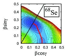
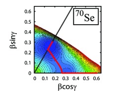
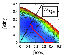
Figure 1: (Color online) The collective paths for ^68-72Se obtaind by the ASCC method. The collective path projected onto the $(\beta,\gamma)$ deformation plane are drawn by solid lines on the potential energy surface. The equipotential lines are drawn every 100 keV. Note that the collective path is symmetric with respect to the reflections about the prolate ($\gamma=0^{\circ}$) and the oblate ($\gamma=60^{\circ}$) axes. The collective path going along the symmetry axis eventually terminates at large $\beta$ when the neutron pairing gap collapses (see the text).

Figure 2: Results of the ASCC calculation for ⁶⁸Se. The monopole pairing gaps $\Delta_{0}^{(\tau)}(q)$, the quadrupole pairing gaps $\Delta^{(\tau)}_{20}(q)$ and $\Delta^{(\tau)}_{22}(q)$, the collective potential $V(q)$, the collective mass $M(s(q))$, the rotational moments of inertia ${\cal J}_{i}(q)$, the lowest two moving-frame QRPA frequencies squared $\omega^{2}(q)$, the axial quadrupole deformation $\beta(q)$, and the canonical collective coordinate $q$ are plotted as functions of $\gamma(q)$.

Figure 3: The same as Fig. 2 but for ⁷⁰Se plotted as functions of $q$ along the collective path. The point $q=0$ corresponds to the prolate local minimum, while the oblate minimum is located at $q=2.18$. These positions are indicated by arrows with $P$ or $O$.

Figure 4: The same as Fig. 2 but for ⁷²Se plotted as functions of $q$ along the collective path. The point $q=0$ corresponds to the oblate minimum, while the prolate local minimum is located at $q=2.34$. These positions are indicated by arrows with $O$ or $P$.

IV.3.1 ⁶⁸Se

In this nucleus, the potential barrier height is about 0.5 and 0.07 MeV measured from the oblate and prolate local minima, respectively. The oblate HB state is chosen as a starting state for solving the ASCC equations. Though the collective path for ⁶⁸Se is already reported in the previous work Hinohara et al. (2008), we summarize the character of the solution of the ASCC equations for later convenience. The collective path starting from the oblate HB states almost follows the triaxial potential valley.

In Fig. 2, we see that the deformation $\beta$ almost stays constant during when the triaxial deformation $\gamma$ changes from $60^{\circ}$ to $0^{\circ}$ along the collective path. This clearly indicates that the triaxial degree of freedom plays much more important role than the axial degree of freedom in ⁶⁸Se. The $\gamma$-dependence of the calculated moments of inertia exhibits a behaviour similar to the irrotational moments of inertia; two of them coincide at the axially symmetric limit while the largest moment of inertia is about the intermediate axis.

In Fig. 2, the collective mass defined as a function of the geometrical length $ds=\sqrt{d\beta^{2}+\beta^{2}d\gamma^{2}}$ in the ($\beta,\gamma$) plane,

$$M(s(q))=B^{-1}(q)\left\{\left(\frac{d\beta}{dq}\right)^{2}+\beta^{2}(q)\left(\frac{d\gamma}{dq}\right)^{2}\right\},$$ (30)

is also presented. As mentioned in Sec. III, we can set $M(q)=B(q)^{-1}=1~{}$MeV^-1 using the units where $\hbar=1$ and the collective variables $(q,p)$ are non-dimensional.

IV.3.2 ⁷⁰Se

In this nucleus, the potential barrier height is about 0.7 and 0.1 MeV measured from the oblate and prolate local minima, respectively. The collective path is obtained starting from the prolate HB state. The two HB local minima are connected by the one-dimensional path. Since the QRPA mode with the lowest frequency at the prolate shape has $\beta$-vibrational character with $K=0$, the collective path starting from the prolate HB state goes along the axial symmetry axis in the beginning. As seen in Figs. 1 and 3, at $q\simeq 0.4~{}(\beta\simeq 0.27)$, the collective path deviates from the $\gamma=0^{\circ}$ line due to the character change of the lowest mode from $K=0$ to $K=2$. To describe such a dynamical breaking of the axial symmetry taking place along the collective path, it is crucial to use Eq. (20) as an initial trial for self-consistently determining the collective coordinate operator $\hat{Q}(q)$. The collective path encounters a similar avoided crossing of the moving-frame QRPA modes at $q\simeq 1.8$ (the oblate side with $\beta\simeq 0.27$). Then, the triaxial path again changes its direction and go along the $\gamma=60^{\circ}$ line. This kind of dynamical breaking of the axial symmetry was previously reported in the analysis of the collective path for ⁷²Kr Kobayasi et al. (2005); Hinohara et al. (2008). At the oblate side of the collective path, the $\beta$-vibrational degrees of freedom strongly couples with the pairing-vibrational degree of freedom of neutrons, and it ends at a large $\beta$ point where the neutron pairing gap collapses. When approaching this point, the collective mass diverges.

As the rotation about the symmetry axis disappear, the moments of inertia ${\cal J}_{3}(q)$ and ${\cal J}_{2}(q)$ should be dropped in the determinant $|G(q)|$ of the metric $G_{mn}(q)$ when the collective path runs along the $\gamma=0^{{}^{\circ}}$ and $\gamma=60^{{}^{\circ}}$ lines, respectively. To avoid discontinuity at the point where the collective path starts to deviate from the symmetry axis, we use $|G(q)|=B^{-1}(q){\cal J}_{1}(q)$ for the whole region of the collective path of this nucleus.

In the region of prolate shape with $\beta>0.34$, the lowest two QRPA modes with $\beta$ and $\gamma$ characters approximately degenerate in energy and compete (see Fig. 3). In such a situation, it may be appropriate to introduce two collective coordinates. In the present calculation, however, we have solved the ASCC equations in this region assuming that the collective path continues to go along the $\gamma=0^{\circ}$ axis. We shall attempt to introduce two collective coordinates in the same framework of the ASCC method in future.

IV.3.3 ⁷²Se

In this nucleus, the potential barrier height is about 0.5 and 0.3 MeV measured from the oblate and prolate local minima, respectively. The collective path is determined starting from the oblate HB state. As seen in Figs. 1 and 4, the collective path directs to the triaxial region because the character of the lowest QRPA mode at the oblate minimum is $\gamma$-vibrational. At $q\simeq 0.2$ in the triaxial region, the collective path curves due to an interplay of the lowest two moving-frame QRPA modes. The collective path reaches the prolate side at $q\simeq 1.6~{}(\beta\simeq 0.32)$. Then the path changes its direction to the $\gamma=0^{\circ}$ line. Thus, the oblate and prolate local minima are connected by a single collective coordinate. After passing through the prolate minimum at $q\simeq 2.1~{}(\beta\simeq 0.38)$, it continues to go along the $\gamma=0^{\circ}$ line and finally terminates at $\beta\simeq 0.42$ where the neutron pairing gap collapses. Correspondingly, the collective mass increases with increasing $\beta$ and finally diverges.

As discussed above for ⁷⁰Se, the moment of inertia ${\cal J}_{3}(q)$ should be dropped in the determinant $|G(q)|$ when the collective path runs along the $\gamma=0^{{}^{\circ}}$ line. Since the collective path for ⁷²Se does not run along the $\gamma=60^{{}^{\circ}}$ line at all, we use $|G(q)|=B^{-1}(q){\cal J}_{1}(q){\cal J}_{2}(q)$ for the whole region of the collective path of this nucleus.

IV.4 Shape mixing, excitation spectra, quadrupole transitions and moments

We have calculated collective wave functions solving the collective Schrödinger equation (25) and evaluated excitation spectra, quadrupole transition probabilities and spectroscopic quadrupole moments. Below we discuss these results denoting the eigenstates belonging to the ground and excited bands as $0_{1}^{+},2_{1}^{+},4_{1}^{+},6_{1}^{+}$ and $0_{2}^{+},2_{2}^{+},4_{2}^{+},6_{2}^{+}$, respectively.

IV.4.1 ⁶⁸Se

In Fig. 5, excitation spectrum and $B$(E2) values calculated for ⁶⁸Se are displayed together with experimental data. It is seen that the calculation yields two bands which exhibit significant deviations from the regular rotational pattern. We note, in particular, that the calculated $0_{2}^{+}$ state is located above the $2_{2}^{+}$ state. This is consistent with the available experimental data where the $0_{2}^{+}$ state has not yet been found. We see in Fig. 6 that the vibrational wave functions of the $0_{1}^{+},0_{2}^{+},2_{1}^{+}$ and $2_{2}^{+}$ states spread over the whole extent of $\gamma$ from the oblate to the prolate shapes. This result of calculation is reasonable considering the very low potential barrier along the triaxial collective path, as we have already seen in Fig. 2. The unusual behavior of the excited $0^{+}$ state noted above suggests that the low-lying states in ⁶⁸Se are in an intermediate situation between the oblate-prolate shape coexistence and the Wilets-Jean $\gamma$-unstable model Wilets and Jean (1956). In fact, we can find a pattern in the calculated E2-transition probabilities, which is characteristic to the $\gamma$-unstable situation; for instance, $B$(E2; $6_{2}^{+}\to 6_{1}^{+}$), $B$(E2; $4_{2}^{+}\to 4_{1}^{+}$) and $B$(E2; $2_{2}^{+}\to 2_{1}^{+}$) are much larger than $B$(E2; $6_{2}^{+}\to 4_{1}^{+}$), $B$(E2; $4_{2}^{+}\to 2_{1}^{+}$) and $B$(E2; $2_{2}^{+}\to 0_{1}^{+}$). This point will be discussed with a more general perspective in a future publication Sato et al. . It is quite interesting to notice that the shape mixing becomes weak as the angular momentum increases, and the collective wave functions of the $4^{+}$ and $6^{+}$ states tend to localize in the region near either the oblate or the prolate shape. Namely, it becomes possible to characterize the $4^{+}$ and $6^{+}$ states as oblate-like or prolate-like.

Figure 5: Theoretical (left) and experimental (right) excitation spectra and $B$(E2) values for low-lying states in ⁶⁸Se. Only $B$(E2)’s larger than 1 Weisskopf unit are shown in units of $e^{2}$ fm⁴. Experimental data are taken from Fischer et al. (2000, 2003).

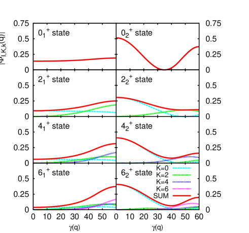
Figure 6: (Color online) Vibrational wave functions $\Phi_{IKk}(q)$ squared of the lowest (left) and the second-lowest states (right) for each angular momentum in ⁶⁸Se. In each panel, different $K$ components of the vibrational wave function and the sum of them are plotted as functions of $\gamma(q)$.

IV.4.2 ⁷⁰Se

Calculated and experimental excitation spectra and $B$(E2) values for ⁷⁰Se are displayed in Fig. 7. The excitation energies of the ground band is well reproduced. The calculated $B$(E2;$2_{1}^{+}\rightarrow 0_{1}^{+}$) value 390 $e^{2}$ fm⁴ is also in reasonable agreement with the experimental data 342 $e^{2}$ fm⁴. The calculated E2-transition probabilities exhibit a pattern somewhat different from that of ⁶⁸Se; for instance, we see significant cross talks among the $2_{1}^{+},2_{2}^{+},4_{1}^{+}$ and $4_{2}^{+}$ states. The vibrational wave functions of the $0_{1}^{+},0_{2}^{+},2_{1}^{+}$ and $2_{2}^{+}$ states displayed in Fig. 8 show strong oblate-prolate shape mixings. In contrast, the $4_{1}^{+}$ and $6_{1}^{+}$ ($4_{2}^{+}$ and $6_{2}^{+}$) states are rather well localized around the prolate (oblate) shape. Thus, the characteristic cross talks of the E2 transition strengths mentioned above are associated with the significant change in localization properties of the vibrational wave functions between angular momenta 2 and 4. Experimental data for such inter- and intra-band $B$(E2) values will certainly serve as a very good indicator of the shape mixing.

Figure 7: The same as Fig. 5 but for ⁷⁰Se. Experimental data are taken from Rainovski et al. (2002); Ljungvall et al. (2008). A candidate of the $0_{2}^{+}$ state is suggested in experiment Ahmed et al. (1981) at about 2 MeV, although it is not drawn.

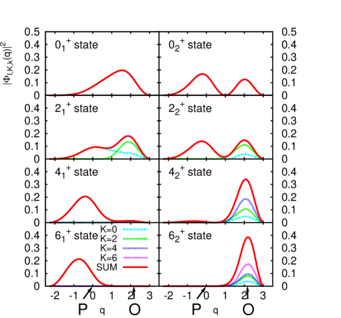
Figure 8: (Color online) Same as Fig. 6 but for ⁷⁰Se. The vibrational collective wave functions squared are plotted as functions of $q$. The arrows indicate the positions of the oblate ($O$) and the prolate ($P$) minima.

IV.4.3 ⁷²Se

Calculated excitation spectrum and $B$(E2) values for ⁷²Se are shown in Fig. 9 together with experimental data. It is seen that the experimental spectrum is reproduced fairly well. The calculated $B$(E2;$2_{1}^{+}\rightarrow 0_{1}^{+}$) value 390 $e^{2}$ fm⁴ is also in good agreement with the experimental data 405 $e^{2}$ fm⁴. We see that the calculated inter-band E2 transitions, $B$(E2; $4_{2}^{+}\to 4_{1}^{+}$), $B$(E2; $4_{2}^{+}\to 2_{1}^{+}$), $B$(E2; $2_{2}^{+}\to 2_{1}^{+}$) and $B$(E2; $4_{1}^{+}\to 2_{2}^{+}$), are reduced from those in ⁷⁰Se, except for $B$(E2; $0_{2}^{+}\to 2_{1}^{+}$).

The vibrational wave functions are displayed in Fig. 10. Similarly to ⁷⁰Se, the $0_{1}^{+}$ wave function widely spreads over the triaxial region. It takes the maximum at the oblate shape, but extends to the prolate region. The $2_{1}^{+}$ wave function also extends the whole region of $\gamma$. In the ground band, the prolate character develops with increasing angular momentum, as clearly seen in the wave functions of the $4_{1}^{+}$ and $6_{1}^{+}$ states.

Dynamical reason why the prolate character of the ground band develop with increasing angular momentum may be understood in terms of the competition between the potential and kinetic energies as function of the collective coordinate $q$. We find that the rotational energy term plays a particularly important role. Because the quadrupole deformation $\beta\simeq 0.38$ at the prolate local minimum is much larger than that ($\beta\simeq 0.27$) at the oblate minimum, the moment of inertia ${\cal J}\simeq 10.3$ MeV^-1 at the former is appreciably larger than ${\cal J}\simeq 6.2$ MeV^-1 at the latter. The difference between the rotational energies at the prolate and oblate minima is easily evaluated to be about 0.19, 0.64, 1.35 MeV for the $2^{+},4^{+},6^{+}$ states, respectively. Therefore, the prolate shape is favoured in order to reduce the rotational energy. As the rotational angular momentum increases, this rotational effect becomes more important and overcomes the small disadvantage in the potential energy. In contrast, for the $0^{+}$ ground state where the rotational effect is absent, the vibrational wave function takes the maximum at the oblate minimum. For the $2_{1}^{+}$ state, the difference of the rotational energies, about 0.19 MeV, is slightly smaller than that of the potential energies, about 0.32 MeV, so that its collective wave function exhibits a transitional character from oblate-like to prolate-like. For the excited states, the vibrational wave functions possess the dominant bumps around the oblate shape, exhibiting at the same time the second bumps around the prolate shape.

Figure 9: The same as Fig. 5 but for ⁷²Se. Experimental data are taken from Palit et al. (2001); Ljungvall et al. (2008).

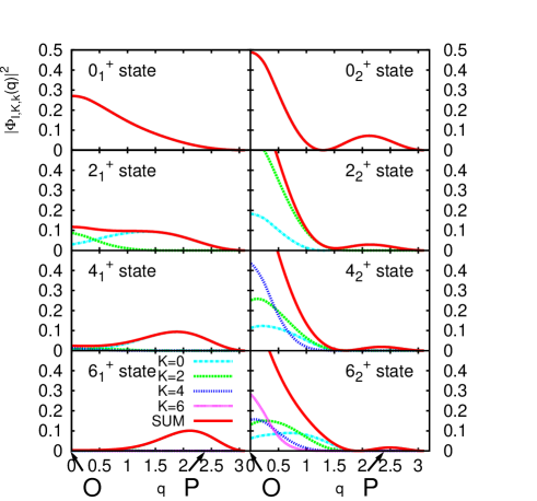
Figure 10: (Color online) Same as Fig. 6 but for ⁷²Se. The vibrational wave functions squared are plotted as functions of $q$. The arrows indicate the positions of the oblate ($O$) and the prolate ($P$) minima.

Figure 11: Spectroscopic quadrupole moments calculated for the low-lying states in ^68,70,72Se. The square, circle and triangular symbols represents those for ⁶⁸Se, ⁷⁰Se and ⁷²Se, respectively. The filled (open) symbols denotes the ground (excited) band.

IV.4.4 Quadrupole moments

The spectroscopic quadrupole moments calculated for ^68,70,72Se are displayed in Fig. 11. For ⁶⁸Se, the $4_{1}^{+}$ and $6_{1}^{+}$ states possess positive signs indicating dominance of the oblate character, while the $4_{2}^{+}$ and $6_{2}^{+}$ states have negative signs indicating dominance of the prolate character. In contrast to the ⁶⁸Se case, the $4_{1}^{+}$ and $6_{1}^{+}$ states in ⁷⁰Se and ⁷²Se have negative signs indicating the growth of prolate character of these states with increasing rotational angular momentum. These results are in qualitative agreement with the HFB-based configuration-mixing calculation reported by Ljungvall et al. Ljungvall et al. (2008). Both calculations indicate the oblate (prolate) dominance for the ground (excited) band in ⁶⁸Se while the prolate character develops with increasing angular momentum for the ground bands in ⁷⁰Se and ⁷²Se. For the excited bands of ⁷⁰Se and ⁷²Se, results of the configuration-mixing calculation are not reported in Ref. Ljungvall et al. (2008). Our calculation indicates the growth of oblate character for the the $4_{2}^{+}$ and $6_{2}^{+}$ states in these isotopes.

Careful interpretation is necessary when absolute values of the calculated spectroscopic quadrupole moment are small. In our results of calculation, small values have nothing to do with spherical character of the states of interest; it is a particular consequence of large-amplitude shape vibration. Namely, we find a number of situations where the contributions from the components of the vibrational wave function with $\gamma>30^{\circ}$ are largely canceled with those from $\gamma<30^{\circ}$. Such a cancellation is the main reason why the calculated quadrupole moments are rather small for all the $2_{1}^{+}$ and $2_{2}^{+}$ states of interest.

IV.4.5 Discussion

Before concluding, we remark on a few questions to be examined in a future publication.

In this paper, we have taken into account the function $G(q)$ in the volume element (29) while it was put unity in the previous calculation Hinohara et al. (2008). Thus, we have obtained, for instance, different ordering between the $0_{2}^{+}$ and $2_{2}^{+}$ states for ⁶⁸Se from that in Ref. Hinohara et al. (2008). This indicates importance of proper treatment of the volume element. In numerical calculations for ⁷⁰Se and ⁷²Se, however, the volume element was treated in an approximate way. We plan to examine the validity of this approximation by deriving a five-dimensional quadrupole collective Hamiltonian on the basis of the ASCC method and make a detailed comparison of the present results with those of the five-dimensional calculation Sato et al. .

Another question is the validity of evaluating the rotational moment of inertia after determining the collective path, Obviously, the assumption that the collective path does not change due to the rotational motion will be eventually violated with increasing angular momentum. Namely, the present approach may be valid only for low-spin states. We have therefore restricted our calculation to low-spin states with angular momentum $I\leq 6$. By comparing with the five-dimensional calculation mentioned above, we shall be able to examine also the range of applicability of the present approach. Alternatively, one can use the rotating mean field when determining the collective path. Such an approach was once tried in Refs. Almehed and Walet and Almehed and Walet (2004).

V Conclusions

Using the ASCC method we have investigated the oblate-prolate shape coexisting/mixing phenomena in proton-rich selenium isotopes, ^68,70,72Se. The collective paths connecting the oblate and prolate HB local minimum were successfully determined. Requantizing the collective Hamiltonian obtained by means of the ASCC method, we have derived the quantum collective Hamiltonian which describes the large-amplitude shape vibration along the collective path and the three-dimensional rotational motion in a unified manner. Solving the collective Schrödinger equation, we have calculated excitation spectra, E2 transition probabilities and spectroscopic quadrupole moments. It has been shown that the basic properties of the coexisting two rotational bands in low-lying states of these nuclei are well reproduced.

The result of calculation clearly shows that the oblate-prolate shape mixing becomes weak as the rotational angular momentum increases. We have analyzed dynamical origin of this trend and found that the rotational energy plays a crucial role in determining the degree of localization of the collective wave function in the $(\beta,\gamma)$ deformation space. The rotational effect causing the localization of the collective wave function may be called “rotational hindrance of shape mixing.” To our knowledge, importance of such a dynamical effect has not been received enough attention in connection with the oblate-prolate shape coexistence phenomena of interest. The rotational hindrance effect will be discussed with a more general perspective in a future publication Sato et al. .