Traffic fluctuations on weighted networks

Abstract

Traffic fluctuation has so far been studied on unweighted networks. However many real traffic systems are better represented as weighted networks, where nodes and links are assigned a weight value representing their physical properties such as capacity and delay. Here we introduce a general random diffusion (GRD) model to investigate the traffic fluctuation in weighted networks, where a random walk’s choice of route is affected not only by the number of links a node has, but also by the weight of individual links. We obtain analytical solutions that characterise the relation between the average traffic and the fluctuation through nodes and links. Our analysis is supported by the results of numerical simulations. We observe that the value ranges of the average traffic and the fluctuation, through nodes or links, increase dramatically with the level of heterogeneity in link weight. This highlights the key role that link weight plays in traffic fluctuation and the necessity to study traffic fluctuation on weighted networks.

I INTRODUCTION

In nature and society, many complex systems can be represented as graphs or networks, where nodes represent the elementary units of a system and links stand for the interactions between the nodes. Complex networks have been a research focus in the last decade  PRL863200 ; PRE66065102 ; PRL91148701 ; PRE69036102 ; PRE71026125 ; PRE65026139 ; RMP7447 ; AP511079 ; SIAMR45167 ; PR424175 .

Recently attention has been given to the traffic fluctuation problem in networks. It is associated with an additive quantity representing the volume of traffic travelling through a node (or a link) in a time interval, and the dependence between its mean and standard deviation Nature189732 . Knowledge on traffic fluctuation is relevant to the design and engineering of real systems such as air transport network, highway network, power-grid network and the Internet, for example how to deploy network resources, how to route traffic efficiently and how to mitigate congestion.

In recent years there has been a strong research interest in the traffic fluctuation problem, which is relevant to a wide range of applications in various networked systems PRL92028701 ; PRL93068701 ; PRL96218702 ; PRL100208701 ; IJBC172363 ; AP5789 . In particular researchers are interested in the relation between the mean of traffic $\langle f\rangle$ and the standard deviation $\sigma$ at a given node. This is because various problems of immediate social and economical interests are ultimately constrained by the extent to which the assignment of resources matches supply and demand under realistic conditions, and the resource assignment is essentially governed by the ‘normal’ traffic behaviour characterised by large fluctuations.

In many real systems, traffic fluctuations are often affected by specific physical properties of network elements, such as the bandwidth of a cable or the computational power of an Internet router. Such systems are much better described as a more sophisticate form of network graphs, the weighted networks, where the physical properties of network elements are represented by link’s weight and node’s strength.

In this paper we investigate the traffic fluctuation problem in weighted networks. In Section II, we review the previous works on traffic fluctuations in unweighted networks. In Section III, we introduce some network properties related to our work and define a number of variables that are used in the study of traffic fluctuation. We introduce a general random diffusion (GRD) model, where a general random walker’s choice of path is affected by link’s weight. In Section IV and V, we analyse the fluctuation of traffic in weighted networks. We provide analytical solutions on the relation between the fluctuation and the average traffic at nodes in section IV and on links in section V. We also run numerical simulations, which confirm our analysis and illustrate its physical meaning. We summarize our work in Section VI.

Our contributions are four folders. Firstly, we introduce a more general analytical law which characterises the traffic fluctuation on weighted networks. Previous works are a special case of our law. Secondly, our results show that traffic fluctuations on a weighted network can be dramatically different from that on the equivalent unweighted network. This highlights the necessity of studying real systems as weighted networks when network elements have a non trivial impact on traffic dynamics. Thirdly, in addition to traffic fluctuation through nodes, we also analytically study traffic fluctuations through links. We show that on weighted networks the traffic fluctuation on links is significant and should be considered when designing real systems. Finally, we reveal the dependence between a link’s traffic properties and the connectivity of the link’s two end nodes.

II Previous Studies on Traffic Fluctuations

The early discovery was that the average volume of traffic arriving at a node, $\langle f\rangle$, and the fluctuation (standard deviation) of the traffic, $\sigma$, follow a power-law relation, i.e. $\sigma\sim\langle f\rangle^{\alpha}$, where the exponent $\alpha$ has two universal values, 1/2 and 1 PRL92028701 ; PRL93068701 . This result has attracted a lot of interest from the network research community and it also generated debates. Subsequently, it has been shown numerically that there is a wide spectrum of possible values within the range of $[1/2,1]$ for $\alpha$ PRL96218702 .

Next, Kujawski et al NJP9154 revealed some scaling properties of traffic fluctuation by conducting simulations on unweighted scale-free networks, where a navigation algorithm is used to give a preference for less used edges in the traffic history. However the scenario considered in NJP9154 is unrealistic. because if an edge is less used in a network’s traffic history, it indicates that the edge is indeed not preferred, for reasons like smaller capacity, longer delay or more expensive.

Recently, Meloni et al PRL100208701 derive an analytical law showing that the dependence of fluctuations with the mean traffic on unweighted networks. They point out the dependence of fluctuations with the mean traffic is governed by the delicate interplay of three factors: the size of observation window; the noise associated to the fluctuations in the number of packets from time window to time window; the degree of the node. However, unweighted networks are relatively simple and widely used to represent the connectivity structure of a network system. On an unweighted network, physical properties of links (and nodes) are removed such that all links are equal, i.e. each link only represents the existence of a topological connection between two nodes.

As is known, many real systems display different interaction strengths between nodes, which reveal unweighted networks’ drawback in link definition. In this case, it is easy to realize that traffic path is rarely randomly chosen. This is because links have different physical properties (bandwidth, delay or cost) and naturally traffic tends to choose a path to achieve better performance, higher efficiency or less cost.

III Traffic Fluctuation on Weighted Networks

III.1 Weighted Networks

A more realistic form of networks is the weighted networks PRE70056131 ; PRE70066149 ; PNAS1013747 , where each link is assigned a weight value to denote a physical property of interest, e.g. the bandwidth of a cable or the length of a road; and similarly, each node is assigned a strength, for example, to represent the computational capacity of an Internet router. Weighted networks encode more information and they are a more realistic representation of real systems where individual links (and nodes) are vastly different.

Weighted networks have the advantage to encode information of physical properties of links and nodes. For example in a weighted social network, a link can indicate that two people know each other while the weight of the link can denote how often they meet each other PNAS1013747 ; in a weighted Internet router network, link weight can represent the bandwidth of a cable and node strength can represent the process power of a router NJP10053022 ; in a weighted aviation network, link weight can denote the annual volume of passengers travelling between two airports PNAS1013747 ; and in the weighed metabolic network E. coli, link weight can encode the optimal metabolic fluxes between two metabolites Nature427839 . On the other hand, recently there are some works on random walk based on weighted networks, but they only considered a single random walker PRE77066105 ; PRE80016107 .

In this work we study the traffic fluctuation problem in weighted networks and investigate critical questions such as ‘what are the impact of different capacity of nodes and links on the fluctuation of traffic passing through them?’ ‘can we predict the fluctuation?’ and ‘what are the implications for network resource assignment?’

III.1.1 Link Weight

In network research the degree, $k$, is defined as the number of links a node has. When representing real systems as weighted networks, the weight of a link is often related to degrees of the two end nodes of the link. For example the number of scheduled flights between two airports increases with the number of flights each of the two airports has.

In this case, we define the weight of a link between nodes $i$ and $j$ as

$$w_{ij}=w_{ji}=(k_{i}k_{j})^{\theta},$$ (1)

where $k_{i}$ and $k_{j}$ are degrees of the two nodes, and $\theta$ is the network’s weightiness parameter which characterises the dependence between link weight and the node degrees PNAS1013747 ; Nature427839 ; PRL94188702 . This definition is well supported by empirical studies PNAS1013747 ; Nature427839 ; PRL94188702 and is widely used in researches on weighted networks. It introduces the weightiness parameter which conveniently determines the level of link heterogeneity in a weighted network. When $\theta=0$ there is no dependence between link weight and node degree, all links are equal with $w=1$, and the network becomes an unweighted network. When $\theta>0$, it is a weighted network where links have different weights. The larger $\theta$, and the wider difference between links.

III.1.2 Node Strength

On the other hand, the strength of node $i$ is defined as

$$s_{i}=\sum_{j\in\Gamma(i)}w_{ij}=\sum_{j\in\Gamma(i)}{(k_{i}k_{j})^{\theta}},$$ (2)

where $\Gamma(i)$ is the set of neighbours of node $i$. In an unweighted network with $\theta=0$, $s_{i}=k_{i}$ node strength is the same as node degree. In a weighted network with $\theta>0$, a node’s strength is the sum of the weight of the links connecting to the node. Two nodes with the same degree may have different strength values depending on the weight of their links. For example consider two airports $A$ and $B$, both have 4 flight connections, $k_{A}=k_{B}=4$. Airport $A$ will have more ‘strength’ than airport $B$ if the former is connected with four well-connected hub airports and the later is connected with four less-connected local airports.

III.2 General Random Diffusion (GRD) Model

Random walk is a mathematical formalisation of a trajectory that consists of taking successive random steps. A familiar example is the random walk phenomenon in a liquid or gas, known as Brownian motion AP17549 ; AP21756 . Random walk is also a fundamental dynamic process on complex networks PRL92118701 . Random walk in networks has many practical applications, such as navigation and search of information on the World Wide Web and routing on the Internet PRE63041108 ; PRE64046135 ; PRL89248701 ; PRE74046118 ; PA385743 . Previous research on traffic fluctuation either studied random walkers travelling on unweighted networks where the choice of route is random as all links are regarded as equal PRL92028701 ; PRL93068701 ; PRL96218702 ; PRL100208701 , or examined a single random walker travelling on weighted networks PRE77066105 ; PRE80016107 .

Before introducing our model, we firstly introduce the general random walk on weighted networks. Let’s consider a general random walker starting from node $i$ at time step $t=0$ and denote $P_{im}(t)$ as the probability of finding the walker at node $m$ at time $t$. The probability of finding the walker at node $j$ at the next time step is $P_{ij}(t+1)=\sum_{m}a_{mj}\cdot\Pi_{m\rightarrow j}\cdot P_{im}(t)$, where $a_{mj}$ is an element of the network’s adjacent matrix. Here, $\Pi_{m\rightarrow j}$ is defined as $\frac{w_{mj}}{s_{m}}$.

Thus the probability $P_{ij}(t)$ for the walker to travel from node $i$ to node $j$ in $t$ time steps is

$$P_{ij}(t) = \sum_{m_{1},...,m_{t-1}}\frac{a_{im_{1}}w_{im_{1}}}{s_{i}}\times\frac{a_{m_{1}m_{2}}w_{m_{1}m_{2}}}{s_{m_{1}}}$$ (3)

$$\times \ldots\times\frac{a_{m_{t-1}j}w_{m_{t-1}j}}{s_{m_{t-1}}}.$$

In other words, $P_{ij}(t)=\sum_{m_{1},...,m_{t-1}}P_{im_{1}}P_{m_{1}m_{2}}\cdot\cdot\cdot P_{m_{t-1}j}$. Comparing the expressions for $P_{ij}$ and $P_{ji}$ one can see that $s_{i}P_{ij}(t)=s_{j}P_{ji}(t)$. This is a direct consequence of the undirectedness of the network. For the stationary solution, one obtains $P_{i}^{\infty}={s_{i}}/{Z}$ with $Z=\sum_{i}s_{i}$. Note the stationary distribution is, up to normalization, equal to $s_{i}$, the strength of the node $i$. This means the higher strength a node has, the more often it will be visited by a walker.

Here we propose the general random diffusion (GRD) model, which describes the traffic fluctuation problem as a large number of independent random walkers travelling simultaneously on a weighted network, where a walker’s choice of path is based on the rule mentioned above.

III.2.1 Size of time window, $M$

We observe traffic arriving at a node (or passing through a link) in time windows of equal size. Each time window consists of $M$ time units, which is defined as a step for random walkers to hop from one node to another.

III.2.2 Preferential choice of path

A walker at node $i$ chooses link $i$–$j$ as the next leg of travel according to the following preferential probability,

$$\Pi_{i\rightarrow j}=\frac{w_{ij}}{\sum_{j\in\Gamma(i)}w_{ij}}=\frac{w_{ij}}{s_{i}},$$ (4)

which is proportional to the weight of the link.

III.2.3 Average traffic, $\langle f\rangle$

The traffic arriving at node $i$ during a time window is $f_{i}=\sum_{m=1}^{M}\Delta_{i}(m),$ where $\Delta_{i}(m)$ is a random variable representing the number of walkers arriving at node $i$ at the $m$th time unit. The average traffic, $\langle f_{i}\rangle$, is the mean traffic volume at node $i$ over all time windows. Similarly, $f_{ij}$ is the traffic passing through a link between nodes $i$ and $j$ during a time window, and $\langle f_{ij}\rangle$ is the average link traffic.

III.2.4 Traffic fluctuation, $\sigma$

The standard deviation $\sigma_{i}$ indicates the fluctuation of traffic volume around the average traffic $\langle f_{i}\rangle$ at node $i$ over time windows. Similarly $\sigma_{ij}$ is the fluctuation of link traffic $f_{ij}$ on the link between nodes $i$ and $j$.

The key interest on the traffic fluctuation problem is the relation between the average traffic $\langle f\rangle$ (of a node or link) and the fluctuation $\sigma$, and the impact of relevant quantities (time window size $M$, weightiness parameter $\theta$ and node degree $k$) on such relation. In the following two sections we investigate traffic fluctuation of node and link respectively.

IV Node Traffic Fluctuation on Weighted Networks

IV.1 Analytical Solution

According to the GRD model’s preferential choice of path (see 4), in the stationary regime the number of walkers visit node $i$ at a single time step can be estimated as

$$\Phi_{i}(r)=r\frac{s_{i}}{\sum_{i=1}^{N}s_{i}},$$ (5)

where $r$ is the number of random walkers travelling on the weighted network and $N$ is the number of nodes. In the GRD model random walkers are independent and the arrival of walkers at a node is a Poisson process. Thus the mean number of walkers visit node $i$ in a window of $M$ time steps is

$$\langle f_{i}\rangle=\Phi_{i}(r)M,$$ (6)

and the probability that exactly $n$ walkers visit node $i$ in a time window is

$$P_{i}(n)=e^{-\Phi_{i}(r)M}\frac{[\Phi_{i}(r)M]^{n}}{n!}.$$ (7)

In a more general case, the number of walkers $r$ observed from time window to time window is uniformly distributed in $[R-\delta,R+\delta]$, $0<\delta\leq R$, where $R$ is the average number of walkers and the noise constant $\delta$ is the fluctuation. The probability of having $r$ walkers in a time window is

$$F(r)=\frac{1}{2\delta+1}.$$ (8)

Then (7) becomes the following

$$\psi_{i}(n) = \sum_{j=0}^{2\delta}(\frac{e^{-(s_{i}/\sum_{i=1}^{N}s_{i})(R-\delta+j)M}}{2\delta+1}$$

$$\times \frac{[(s_{i}/\sum_{i=1}^{N}s_{i})(R-\delta+j)M]^{n}}{n!}).$$

Calculating the first and second moments of $f_{i}$, we get

$$\langle f_{i}\rangle=\sum_{n=0}^{\infty}n\psi_{i}(n)=\frac{s_{i}}{\sum_{i=1}^{N}s_{i}}RM$$ (10)

and

$$\langle{f^{2}_{i}}\rangle=\sum_{n=0}^{\infty}n^{2}\psi_{i}(n)={\langle f_{i}\rangle}^{2}\left(1+\frac{\delta^{2}+\delta}{3R^{2}}\right)+{\langle f_{i}\rangle}.$$ (11)

Then the standard deviation as a function of $\langle f_{i}\rangle$ is

$${\sigma^{2}_{i}}=\langle f_{i}\rangle\left(1+\langle f_{i}\rangle\frac{\delta^{2}+\delta}{3R^{2}}\right).$$ (12)

This indicates the relation between the traffic at nodes and its scale doesn’t depend on the weight parameter $\theta$. The traffic fluctuation at node $i$ can be given as $\sigma_{i}^{2}=(\sigma^{\rm int}_{i})^{2}+(\sigma^{\rm ext}_{i})^{2}$. This suggests that the driving force of traffic fluctuation at node $i$ can be ascribed to two aspects: one is the internal randomness of the diffusion process, $\sigma^{\rm int}_{i}=\sqrt{\langle f_{i}\rangle}$; and the other is the change in the external environment, $\sigma^{\rm ext}_{i}=\langle f_{i}\rangle\sqrt{\frac{\delta^{2}+\delta}{3R^{2}}}$, i.e. the fluctuation of the number of walkers in the network in different time windows. To make it concrete, we will show a class of specifical networks to testify its validity in what follows.

IV.1.1 For Neutral Weighted Networks

Networks exhibit different mixing patterns, or degree-degree correlations PRL89208701 ; PRE67026126 . For example social networks show the assortative mixing where high-degree nodes tend to connect with other high-degree nodes and low-degree nodes with low-degree ones. By contrast, biological and technological networks show the disassortative mixing where high-degree nodes tend to connect with low-degree nodes and vice versa.

Neutral networks show neither assortative nor disassortative mixing. Three popular examples are (1) the Erdös-Rényi (ER) random graph PM6290 , which is generated by random link attachment between nodes and is characterised by a Poisson degree distribution; (2) the Barabási-Albert (BA) scale-free graph SCI286509 , which is generated by the so-called preferential attachment and is characterised by a power-law degree distribution; and (3) the Watts-Strogatz (WS) small-world NATURE393440 is generated by rewiring links on regular lattices and is characterised by a high clustering SIAMR45167 and a small average topological distance PRE70056110 . These three generic models have been widely studied in network research.

IV.1.2 Node Strength Expressed As Node Degree

$P(k_{q}|k_{i})$ is the conditional probability distribution that a $k_{q}$-degree node connects with a $k_{i}$-degree node PRL89208701 . For neutral networks,

$$P(k_{q}|k_{i})=P(k_{q}|k)=k_{q}P(k_{q})/\langle k\rangle,$$ (13)

where $P(k_{q})$ is the probability of a node having degree $k_{q}$ and $\langle k\rangle$ is the average degree PRL89208701 .

The nearest-neighbours average degree of node $i$ can be estimated as ${{k_{nn}(k_{i})}}=\sum_{k_{q}=k_{min}}^{k_{max}}{k_{q}}P(k_{q}|k_{i}),$ where suffix $q$ stands for a neighbor of node $i$, $k_{min}$ and $k_{max}$ are the minimum and maximal node degrees in the network, respectively. By mean-field approximation we have

$${{k^{\theta}_{nn}(k_{i})}}=\sum_{k_{q}=k_{min}}^{k_{max}}k_{q}^{\theta+1}P(k_{q})/\langle k\rangle=\langle k^{\theta+1}\rangle/\langle k\rangle.$$ (14)

One can see that ${k_{nn}^{\theta}}(k_{i})$ does not depend on the degree $k_{i}$, hence $\sum_{q\in\Gamma(i)}{k_{q}^{\theta}}=k_{i}\cdot{k^{\theta}_{nn}(k_{i})}$. Using Eqs. (2) and (14) we have

$$s_{i}={k^{\theta+1}_{i}}{\langle k^{\theta+1}\rangle}/{\langle k\rangle}.$$ (15)

For neutral weighted networks, we can then rewrite (10) as

$$\langle f_{i}\rangle=\frac{k^{\theta+1}_{i}}{N\langle k^{\theta+1}\rangle}RM.$$ (16)

When the four quantities $M$, $R$, $\delta$ and $\theta$ satisfy the condition that $\frac{\delta^{2}+\delta}{3R}\cdot\frac{k_{i}^{\theta+1}}{N\langle k^{\theta+1}\rangle}M\ll 1$, the relation between traffic fluctuation and average traffic as given in (12) is reduced to a power-law scaling $\sigma\sim{\langle f\rangle}^{\alpha}$ with $\alpha=1/2$. When $\frac{\delta^{2}+\delta}{3R}\cdot\frac{k_{i}^{\theta+1}}{N\langle k^{\theta+1}\rangle}M$ is not negligible, the exponent $\alpha$ is in the range of $[1/2,1]$.

IV.2 Numerical Simulation

We run numerical simulations for the following purpose: (1) to verify the analytical solution; (2) to examine the impact of parameters such as window size $M$ and node degree $k$ on the power-law scaling of the traffic fluctuation function; and (3) to contrast unweighted networks with $\theta=0$ against weighted networks with $\theta>0$.

IV.2.1 Simulation Settings

Our simulation is based on network graphs generated by the BA model SCI286509 , which is neutral mixing and features a power-law degree distribution $P(k)\sim k^{-3}$. We generate ten BA graphs, each of which has 5,000 nodes and 25,000 links. We assign link weight and node strength as defined in (1) and (2) respectively. Initially, we disperse $r=R\pm\delta=10,000\pm 1,000$ random walkers uniformly on nodes. At each time step, all walkers travel one hop according to (4). For a given time window size of $M$, we observe traffic fluctuation at each node over a large number of time windows.

For each given value of time window size $M$ or weightiness parameter $\theta$, we repeat the simulation for 50 times (with different random seeds) on each of the ten BA networks. Each result shown below is averaged over the $10\times 50=500$ simulations.

IV.2.2 Power-Law Relation Between $\sigma_{i}$ and $\langle f_{i}\rangle$

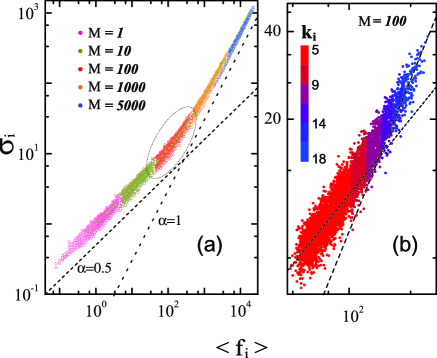
Figure 1: Traffic fluctuation $\sigma_{i}$ as a function of average traffic $\langle f_{i}\rangle$ at node $i$. (a) Observed in different time window sizes of $M=1,10,100,1000$ and 5000; and (b) for nodes of different degrees (with $M=100$). The green dotted-line in (a) is the analytical solution given in (12). The two black dotted-lines in both (a) and (b) correspond to $\sigma_{i}\sim\langle f_{i}\rangle^{\alpha}$ with $\alpha=0.5$ and 1, respectively. Simulation results are obtained on weighted BA networks having 5,000 nodes and 25,000 links with the weightiness parameter $\theta=0.5$, the average number of random walkers $R=10^{4}$ and the noise constant of $\delta=10^{3}$. For clarity we only show nodes with degrees smaller than 18. Note that the minimal degree in the networks is 5 as $m_{0}=5$ and $m=5$ in the weighted BA networks.

Figure 1(a) shows the relation between traffic fluctuation $\sigma$ and average traffic $\langle f\rangle$ for different time window size $M$ where the weightiness parameter is set as $\theta=0.5$. The simulation results overlap with the analytical solution. Both the average traffic and the traffic fluctuation increase with the size of window $M$. For any given value of $M$, the two quantities follow a power-law relation $\sigma\sim\langle f\rangle^{\alpha}$. When $M$ is small, the power-law exponent $\alpha$ is close to $1/2$; and when $M$ increases the exponent grows towards $1$.

Figure 1(b) shows the enlargement of the traffic fluctuation function for the window size $M=100$ as circled out in Figure 1(a), where data dots are coloured by node degrees. For nodes with the higher degree, the large values of $\sigma$ and $\langle f\rangle$ are observed. For low-degree nodes (e.g. $k=5$) the power-law exponent is close to $\alpha=1/2$; whereas for higher degree nodes (e.g. $k=18$), the exponent approaches to $1$.

As predicted by Eq. (16), our simulation results confirm that the traffic fluctuation function $\sigma\sim{\langle f\rangle}^{\alpha}$ does not follow a simple power-law. Rather, the power-law scaling is in the range of [1/2, 1]. It is affected by a number of parameters including the window size $M$ and the degree of nodes under study. This echoes previous studies as their random diffusion model based on unweighted networks is a special case of our general random diffusion model on weighted networks.

IV.2.3 Impact of Weightiness Parameter $\theta$

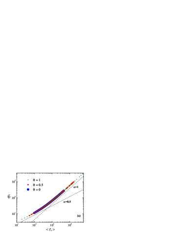
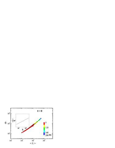
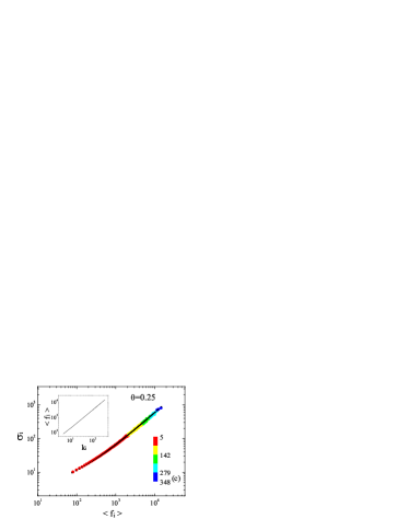
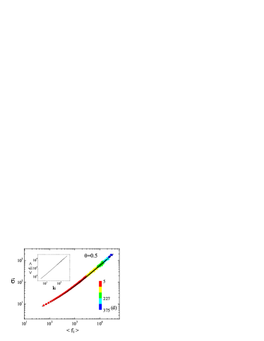
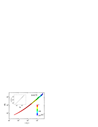
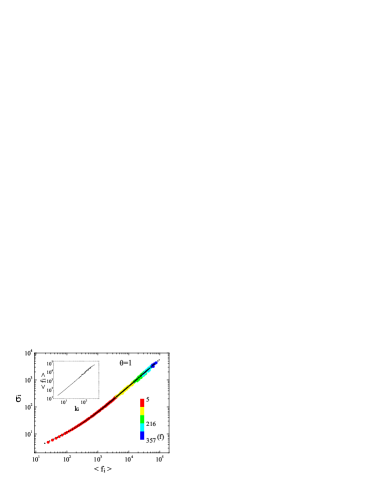
Figure 2: Traffic fluctuation $\sigma_{i}$ as a function of average traffic volume $\langle f_{i}\rangle$ at node $i$ for different values of weightiness parameter $\theta$. (a) shows analytical solutions of (12) for $\theta=0$, 0.5, and 1; and (b), (c), (d), (e) and (f) show simulation results for $\theta=0$, 0.25, 0.5, 0.75, and 1 respectively, where results are shown for all nodes and coloured by node degree $k_{i}$, and the black dotted lines are the analytical solutions. Time window size $M$ is set as 100 and other parameters are as before. The insets of (b), (c) and (d) show $\langle f_{i}\rangle$ as a function of $k_{i}$ on a log-log scale, which is predicted by (16).

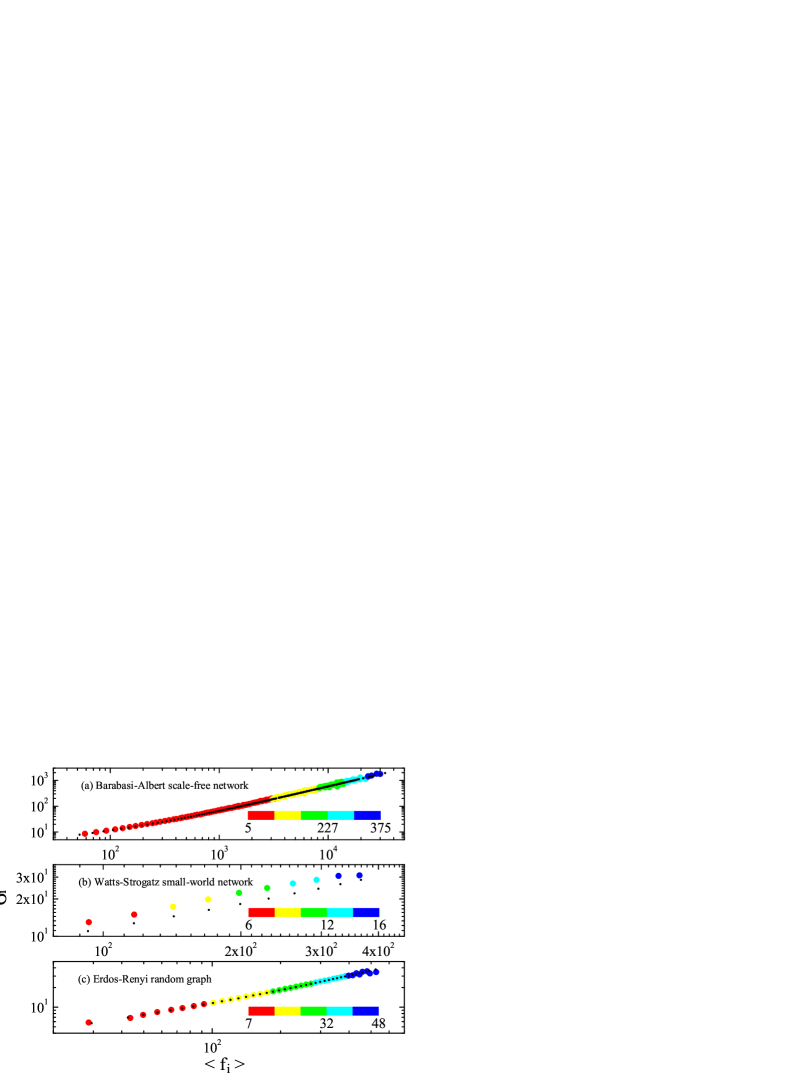
Figure 3: Traffic fluctuation $\sigma_{i}$ as a function of average traffic volume $\langle f_{i}\rangle$ at node $i$ for neutral networks with $\theta=0.5$, $M=100$, $R=10^{4}$ and $\delta=10^{3}$. The black dotted lines are the analytical solution given by (12) and (16). (a) shows the simulation obtained on weighted BA networks with 5,000 nodes and 25,000 links. (b) shows the simulation obtained on weighted Watts-Strogatz small-world networks with rewiring probability 0.1, 5,000 nodes and 25,000 links. (c) shows the simulation obtained on weighted Erdös-Rényi random graphs with connected probability 0.002, 5,000 nodes and 25,000 links.

Figure 2(a) illustrates the solutions of (12) for the weightiness parameter $\theta=0$, 0.5 and 1 with the time window size is set as $M=100$. Figure 2(b), (c), (d), (e) and (f) show the simulation results for $\theta=0$, 0.25, 0.5, 0.75, and 1 respectively. For different $\theta$ values, the traffic fluctuation curves overlap with each other, and in all cases the high-degree nodes are concentrated at the upper-right end of the curves whereas the low-degree nodes are dispersed alone the lower-left part of the curve. The remarkable difference, however, is that with the increase of $\theta$ the value ranges of $\langle f_{i}\rangle$ and $\sigma_{i}$ expand significantly towards both directions. This means that comparing with an unweighted network, traffic fluctuation in a weighted network is more acute at high-degree nodes and more stable at low-degree nodes. This is because in a weighted network the node strength $s\sim k^{\theta+1}$ (see (15)) and therefore high-degree nodes deprive more traffic from low-degree ones than in an unweighted network.

IV.2.4 For Neutral Weighted Networks

Figure 3 shows the simulation results on weighted BA, Watts-Strogatz small-world NATURE393440 networks and Erdös-Rényi random graphs with $\theta=0.5$. As shown in the panels (a) and (c), the simulation results on the scale of $f_{i}$ is remarkably consistent with the solution given by Eq. 12. However, one can find that the numerical results in the panel (b) deviate from Eq. 12 apparently. This deviation is due to most of the links (at least $80\%$ in our simulations) in the small-world networks are still regularly connected. $80\%$ is predicted by the small rewiring probability $0.1$. Obviously, the conditional probability distribution $P(k_{q}|k_{i})$ doesn’t completely match Eq. 13.

Our results suggest that if a real system should be described as a weighted network with $\theta=1$ but instead an unweighted network with $\theta=0$ is used, then we would underestimate the $\langle f_{i}\rangle$ and $\sigma_{i}$ values for high-degree nodes and overestimates the values for low-degree nodes by as large as one order of magnitude. This highlights the importance of choosing a proper network model for traffic fluctuation research.

V Link Traffic Fluctuation on Weighted Networks

V.1 Analytical Solution

In GRD model, random walkers on a weighted network travel independently and therefore the number of walkers passing through a link is a Poisson process. As given in (4), the probability that a walker at node $i$ chooses link $i$–$j$ as the next leg of travel is ${w_{ij}}/s_{i}$. Thus for $r$ random walkers in a weighted network, the average number of walkers passing through link $i$–$j$ (from node $i$ to node $j$ as well as from node $j$ to node $i$) during a time window $M$ is

$$\langle f_{ij}\rangle=\Omega_{ij}(r)M$$

where

$$\Omega_{ij}(r)=r\left(\frac{s_{i}}{\sum_{i=1}^{N}s_{i}}\cdot\frac{w_{ij}}{s_{i}}+\frac{s_{j}}{\sum_{i=1}^{N}s_{i}}\cdot\frac{w_{ij}}{s_{j}}\right),$$ (17)

and the probability of $f_{ij}=n$ in a time window is

$$Q_{ij}(n)=e^{-\Omega_{ij}(r)M}\frac{[\Omega_{ij}(r)M]^{n}}{n!}.$$ (18)

Similar as the above analysis on node traffic fluctuation, for a more general case where the number of random walkers $r$ from time window to time window is distributed in $[R-\delta,R+\delta]$, the probability of $f_{ij}=n$ in a time window is

$$\Gamma_{ij}(n) = \sum_{j=0}^{2\delta}(\frac{e^{\frac{2w_{ij}}{\langle k^{\theta+1}\rangle^{2}N}(R-\delta+j)M}}{2\delta+1}$$

$$\times \frac{e^{\frac{2w_{ij}}{{\langle k^{\theta+1}\rangle}^{2}N}(R-\delta+j)M}}{n!}).$$

Calculating the first and second moments of $f_{ij}$, we obtain

$$\langle f_{ij}\rangle=\sum_{n=0}^{\infty}n\Gamma_{ij}(n)=\frac{2w_{ij}}{\sum_{i=1}^{N}s_{i}}RM,$$ (20)

and

$$\langle f^{2}_{ij}\rangle=\sum_{n=0}^{\infty}n^{2}\Gamma_{ij}(n)={\langle f_{ij}\rangle}^{2}\left(1+\frac{\delta^{2}+\delta}{3R^{2}}\right)+{\langle f_{ij}\rangle}.$$ (21)

Thus the standard deviation as a function of the average traffic $\langle f_{ij}\rangle$ is

$${\sigma^{2}_{ij}}=\langle f_{ij}\rangle\left(1+\langle f_{ij}\rangle\frac{\delta^{2}+\delta}{3R^{2}}\right).$$ (22)

This indicates the relation between the traffic on links and its scale is irrelevant to $\theta$ as well. For neutral weighted networks, using Eqs. (1) and (15), we can rewrite (20) as

$$\langle f_{ij}\rangle=\frac{2(k_{i}k_{j})^{\theta}\langle k\rangle MR}{{\langle k^{\theta+1}\rangle}^{2}N}.$$ (23)

If $\frac{\delta^{2}+\delta}{3R}\cdot\frac{2(k_{i}k_{j})^{\theta}\langle k\rangle M}{{\langle k^{\theta+1}\rangle}^{2}N}\ll 1$, (22) is reduced to a power-law scaling $\sigma_{ij}\sim{\langle f_{ij}\rangle}^{\alpha}$ with $\alpha=1/2$. Conversely, as $\frac{\delta^{2}+\delta}{3R}\cdot\frac{2(k_{i}k_{j})^{\theta}\langle k\rangle M}{{\langle k^{\theta+1}\rangle}^{2}N}$ increases to $1$, the exponent $\alpha$ will leave $1/2$ for $1$.

V.2 Numerical Simulation

Here we use the same simulation settings as Section IV(B).

Figure 4: Traffic fluctuation $\sigma_{ij}$ as a function of average traffic $\langle f_{ij}\rangle$ on link $i$–$j$ between nodes $i$ and $j$ with time window size of $M=10$, 100 and 1000. The green line is the analytical solution given by (22). The black dotted lines correspond to $\sigma_{ij}\sim\langle f_{ij}\rangle^{\alpha}$ with $\alpha=0.5$ and $1$, respectively. The simulation results are obtained on weighted BA networks with 5,000 nodes and 25,000 links with $\theta=0.5$, $R=10^{4}$ and $\delta=10^{3}$.

V.2.1 Power-Law Relation Between $\sigma_{ij}$ and $\langle f_{ij}\rangle$

In Figure 4 we plot the relation between the traffic fluctuation $\sigma_{ij}$ and the average traffic $\langle f_{ij}\rangle$ on link $i$–$j$ for three different values of time window size $M$. The simulation results are in agreement with our analytical solution. As predicted by Eqs. (22) and (23), the average traffic and the fluctuation increase with $M$. The two quantities follow a power-law scaling $\sigma_{ij}\sim{\langle f_{ij}\rangle}^{\alpha}$, where the exponent $\alpha$ is $1/2$ for small value of $M$ and approaches to 1 with larger $M$. Such behaviour is similar as the traffic fluctuation on nodes.

V.2.2 Impact of Weightiness Parameter $\theta$

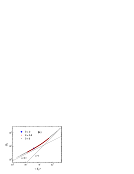
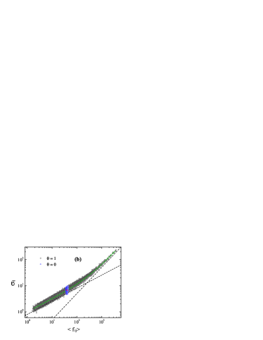
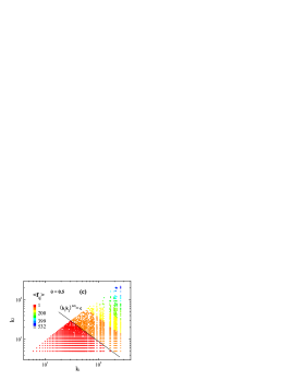
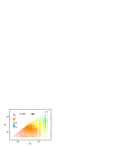
Figure 5: Traffic fluctuation $\sigma_{ij}$ and average traffic $\langle f_{ij}\rangle$ on link $i$–$j$ with parameters $M=100$, $R=10^{4}$ and $\delta=10^{3}$. (a) Shows analytical solutions of (22) for $\theta=0$, 0.5 and 1, respectively. (b), (c) and (d) are simulation results. (b) shows $\sigma_{ij}$ as a function of $\langle f_{ij}\rangle$ for $\theta=0$ and 1. (c) shows the average traffic $\langle f_{ij}\rangle$ on link $i$–$j$ as a function of degrees of the two end nodes of the link, $k_{i}$ and $k_{j}$, where $\theta=0.5$, the value of $\langle f_{ij}\rangle$ is given by a colour bar, and the guideline is given by (23). Similarly (d) shows the traffic fluctuation $\sigma_{ij}$ as a function of $k_{i}$ and $k_{j}$.

Figure 6: Traffic fluctuation $\sigma_{ij}$ and average traffic $\langle f_{ij}\rangle$ on link $i$–$j$ with parameters $M=100$, $R=10^{4}$ and $\delta=10^{3}$. The black dotted lines are the analytical solution given by (22) and (23). (a) shows the simulation obtained on weighted BA networks with 5,000 nodes and 25,000 links with $\theta=0.5$, $R=10^{4}$ and $\delta=10^{3}$. (b) shows the simulation obtained on weighted Watts-Strogatz small-world networks with a rewiring probability 0.1, 5,000 nodes and 25,000 links. (c) shows the simulation obtained on weighted Erdös-Rényi random graphs with connected probability 0.002, 5,000 nodes and 25,000 links.

In Figure 5(a), the range of scale for $\theta=1$ is $[0.5031,0.9602]$ while for $\theta=0$ it is nearly $0$. For $\theta=0$, the links in the simulation form a dense group on the plot NJP9154 , representing almost equal fluctuation properties. This unaccounted fact can be explained by the solutions of (22) and (23). The dashed lines are guides to the eyes and correspond to $\sigma_{i}\sim{\langle f_{i}\rangle}^{\alpha}$, with $\alpha=1/2$ and $\alpha=1$. The comparison among unweighted networks ($\theta=0$) and weighted ones ($\theta>0$) can be observed in this figure in panel (b). Note that the green and red dots reflect the solution of (22). As shown in the figure, the differences of $f_{ij}$ and $\sigma_{ij}$ for different nodes pairs crop up when $\theta=1$. In fact, this process is not as sudden as it looks.

V.2.3 Node Degree $k$

In Figure 5(c) and (d), we show the middle case of $\theta=0.5$ numerically for different node pairs. As shown in the panel (c), the plots are colored by $f_{ij}$. For all the links, we only focus on the results obtained for pairs of $k_{i}$ and $k_{j}$ (restrict $k_{j}>10$ to enhance the speed of loading figures), where $k_{i}>k_{j}$. One can easily find that $f_{ij}$ is directly proportional to the product of two ends’ degrees $k_{i}$ and $k_{j}$ when $\theta>0$, while they are almost a constant when $\theta=0$. Likewise, $\sigma_{ij}$’s are directly proportional to $k_{i}k_{j}$ when $\theta=0.5$ as well, but they are rather stable when $\theta=0$ (see panel (b)).

V.2.4 For Neutral Weighted Networks

Figure 6 shows the simulation results on weighted BA, Watts-Strogatz small-world networks and Erdös-Rényi random graphs with $\theta=0.5$. As shown in the panels (a) and (c), the simulation results on the scale of $f_{ij}$ is consistent with the solution given by Eq. 22. In the panel (b), one can find that the numerical results deviate from Eq. 22 again. The behavior confirms our observations in Fig. 6 and the discussion in Section IV.2.4 in another light.

V.3 Discussion

One simple example for the result is that for a traffic network, the traffics on different roads differ, the wider of which can have the larger traffic. At the same time, the roads with heavy loads fluctuate more dramatically, depending on whether it is a rush hour or not. Indeed, the interactions among walkers should not be ignored in the realistic scenarios, e.g., the transport of information packets, signals, molecules, rumours, diseases, to name but a few. Whereas, these interactions vary widely from case to case. For generality, we begin with this simple model to take a step forward in the analytical investigation of the corresponding problems. We believe our rigorous solutions are capable of prompting related studies on interacting walkers in the near future.

VI CONCLUSION

In summary, we investigate the traffic fluctuation problem on weighted networks, which is a more general and realistic representation of real systems. Previous results on nodes are the most simple case of our result. Moreover, comparatively few investigations have been recorded in the literature relative to the fluctuation on links both for unweighted and weighted networks yet.

In this paper, we introduce the general random diffusion (GRD) model, which describe a swarm of random walkers traveling simultaneously on the weighted networks. Based on the model we provide analytic solutions to characterise the relation between the mean traffic and its fluctuation for nodes and for links. We discuss the impact of key parameters on the traffic fluctuation. Key observations include size of time window, node strength, and link weight. To prove the results, we take neutral networks with a specifical link weight definition for example. Our analysis indicates the relation between the traffic and its scale is irrelevant to the weight parameter $\theta$. Simultaneously, we find the scales of traffic on weighted links with $\theta>0$ are much wider than unweighted ones, on which the traffic are rather stable, which is confirmed by analytical prediction with remarkable accuracy. Thus, both simulations and analytic work have suggested that the weight could have an impact on the way in which networks operate, including the way information travels through the network and resource assignment for an efficient performance of communication networks.

One significant observation is that study based on unweighted networks could lead to unrealistic, misleading results, such as same link traffic and fluctuation for all links. Therefore, the GRD model based on weighted network provides a proper platform for future such research.

- (1) R. Pastor-Satorras and A. Vespignani, Phys. Rev. Lett. 86, 3200, (2001).
- (2) A. E. Motter and Y. C. Lai, Phys. Rev. E 66, 065102, (2002).
- (3) K. I. Goh, D. S. Lee, B. Kahng, and D. Kim, Phys. Rev. Lett. 91, 148701, (2003).
- (4) B. Tadić, S. Thurner, and G. J. Rodgers, Phys. Rev. E 69, 036102, (2004).
- (5) L. Zhao, Y. C. Lai, K. Park, and N. Ye, Phys. Rev. E 71, 026125, (2005).
- (6) H. Hong, M. Y. Choi, and B. J. Kim, Phys. Rev. E 65, 026139, (2002).
- (7) R. Albert and A.-L. Barabási, Rev. Mod. Phys. 74, 47, (2002).
- (8) S. N. Dorogvtsev and J. F. F. Mendes, Adv. Phys. 51, 1079, (2002).
- (9) M. E. J. Newman, SIAM Rev. 45, 167, (2003).
- (10) S. Boccaletti, V. Latora, Y. Moreno, M. Chavez, and D.-U. Hwanga, Phys. Rep. 424, 175, (2006).
- (11) L. R. Taylor, Nature 189, 732, (1961).
- (12) M. A. de Menezes and A.-L. Barabási, Phys. Rev. Lett. 92, 028701, (2004).
- (13) M. A. de Menezes and A.-L. Barabási, Phys. Rev. Lett. 93, 068701, (2004).
- (14) J. Duch and A. Arenas, Phys. Rev. Lett. 96, 218702, (2006).
- (15) S. Meloni, J. Gómez-Gardeñes, V. Latora, and Y. Moreno, Phys. Rev. Lett. 100, 208701, (2008).
- (16) B. Tadić, G. J. Rodgers, and S. Thurner, Int. J. Bifurcation and Chaos, 17, 2363, (2007).
- (17) Z. Eisler, I. Bartos, and J. Kertész, Advances in Physics, 57, 89 (2008).
- (18) B. Kujawski, B. Tadić, and G. J. Rodgers, New J. Phys. 9, 154 (2007).
- (19) M. E. J. Newman, Phys. Rev. E 70, 056131, (2004).
- (20) A. Barrat, M. Barthélemy, and A. Vespignani, Phys. Rev. E 70, 066149, (2004).
- (21) A. Barrat, M. Barthélemy, R. Pastor-Satorras, and A. Vespignani, Proc. Natl. Acad. Sci. U.S.A. 101, 3747, (2004).
- (22) D. H. Kim and A. E. Motter, New J. Phys. 10, 053022, (2008).
- (23) E. Almaas, B. Kovács, Z. N. Oltval and A.-L. Barabási, Nature 427, 839, (2004).
- (24) S. Kwon, S. Yoon, and Y. Kim, Phys. Rev. E 77, 066105, (2008).
- (25) A. Fronczak and P. Fronczak, Phys. Rev. E 80, 016107, (2009).
- (26) W. X. Wang, B. H. Wang, B. Hu, G. Yan, and Q. Ou, Phys. Rev. Lett. 94, 188702, (2005).
- (27) A. Einstein, Ann. Phys. (Leipzig) 17, 549, (1905); 19, 371, (1906).
- (28) M. Smoluchowski, Ann. Phys. (Leipzig) 21, 756, (1906).
- (29) J. D. Noh and H. Rieger, Phys. Rev. Lett. 92, 118701, (2004).
- (30) F. Jasch and A. Blumen, Phys. Rev. E 63, 041108, (2001).
- (31) L. A. Adamic, R. M. Lukose, A. R. Puniyani, and B. A. Huberman, Phys. Rev. E 64, 046135, (2001).
- (32) R. Guimerá, A. Díaz-Guilera, F. Vega-Redondo, A. Cabrales, and A. Arenas, Phys. Rev. Lett. 89, 248701, (2002).
- (33) S. Lee, S.-H. Yook, and Yup Kim, Phys. Rev. E 74, 046118, (2006).
- (34) S. Lee, S.-H. Yook, and Yup Kim, Physica A 385, 743, (2007).
- (35) M. E. J. Newman, Phys. Rev. Lett. 89, 208701, (2002).
- (36) M. E. J. Newman, Phys. Rev. E 67, 026126, (2003).
- (37) P. Erdös and A. Rényi, Publ. Math. 6, 290, (1959).
- (38) A.-L. Barabási and R. Albert, Science 286, 509, (1999).
- (39) D. J. Watts and S. H. Strogatz, Nature (London) 393, 440 (1998).
- (40) A. Fronczak, P. Fronczak, and J. A. Hołyst, Phys. Rev. E 70, 056110 (2004).