Multiple Multicasts with the Help of a Relay

Abstract

The problem of simultaneous multicasting of multiple messages with the help of a relay terminal is considered. In particular, a model is studied in which a relay station simultaneously assists two transmitters in multicasting their independent messages to two receivers. The relay may also have an independent message of its own to multicast. As a first step to address this general model, referred to as the compound multiple access channel with a relay (cMACr), the capacity region of the multiple access channel with a “cognitive” relay is characterized, including the cases of partial and rate-limited cognition. Then, achievable rate regions for the cMACr model are presented based on decode-and-forward (DF) and compress-and-forward (CF) relaying strategies. Moreover, an outer bound is derived for the special case, called the cMACr without cross-reception, in which each transmitter has a direct link to one of the receivers while the connection to the other receiver is enabled only through the relay terminal. The capacity region is characterized for a binary modulo additive cMACr without cross-reception, showing the optimality of binary linear block codes, thus highlighting the benefits of physical layer network coding and structured codes. Results are extended to the Gaussian channel model as well, providing achievable rate regions for DF and CF, as well as for a structured code design based on lattice codes. It is shown that the performance with lattice codes approaches the upper bound for increasing power, surpassing the rates achieved by the considered random coding-based techniques.

I Introduction

Consider two non-cooperating satellites each multicasting radio/TV signals to users on Earth. The coverage area and the quality of the transmission is generally limited by the strength of the direct links from the satellites to the users. To extend coverage, to increase capacity or to improve robustness, a standard solution is that of introducing relay terminals, which may be other satellite stations or stronger ground stations (see Fig. 1). The role of the relay terminals is especially critical in scenarios in which some users lack a direct link from any of the satellites. Moreover, it is noted that the relays might have their own multicast traffic to transmit. A similar model applies in the case of non-cooperating base stations multicasting to mobile users in different cells: here, relay terminals located on the cell boundaries may help each base station reach users in the neighboring cells.

Cooperative transmission (relaying) has been extensively studied in the case of two transmitting users, both for a single user with a dedicated relay terminal [1], [2] and for two cooperating users [3]. Extensions to scenarios with multiple users are currently under investigation [2], [5] - [11]. In this work, we aim at studying the impact of cooperation in the setup of Fig. 1 that consists of two source terminals simultaneously multicasting independent information to two receivers in the presence of a relay station. While the source terminals cannot directly cooperate with each other, the relay terminal is able to support both transmissions simultaneously to enlarge the multicast capacity region of the two transmitters. Moreover, it is assumed that the relay station is also interested in multicasting a local message to the two receivers (see Fig. 2).

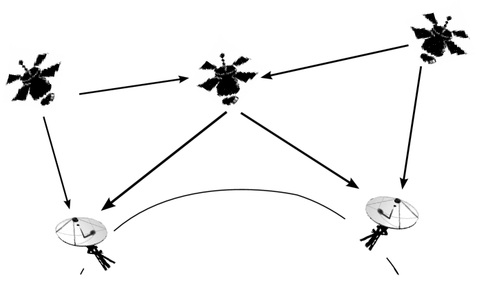
Figure 1: Illustration for an application of the compound multiple access channel with a relay.

The model under study is a compound multiple access channel with a relay (cMACr) and can be seen as an extension of several fundamental channel models, such as the multiple access channel (MAC), the broadcast channel (BC) and the relay channel (RC). The main goal of this work is to adapt basic transmission strategies known from these key scenarios to the channel at hand and to identify special cases of the more general model for which conclusive capacity results can be obtained.

Below, we summarize our contributions:

• We start our analysis by studying a simplified version of the cMACr that consists of a MAC with a “cognitive” relay (see Fig. 3). In this scenario the cognitive relay is assumed to be aware of both transmitters’ messages non-causally. We provide the capacity region for this model and several extensions. While interesting on its own, this setup enables us to conveniently introduce the necessary tools to address the analysis of the cMACr. As an intermediate step between the cognitive relay model and the more general model of cMACr, we also consider the relay with finite capacity unidirectional links from the transmitters and provide the corresponding capacity region.

• We provide achievable rate regions for the cMACr model with decode-and-forward (DF) and compress-and-forward (CF) relaying. In the CF scheme, the relay, instead of decoding the messages, quantizes and broadcasts its received signal. This corresponds to the joint source-channel coding problem of broadcasting a common source to two receivers, each with its own correlated side information, in a lossy fashion, studied in [16]. This result indicates that the pure channel coding rate regions for certain multi-user networks can be improved by exploiting related joint source-channel coding techniques.

• The similarity between the underlying scenario and the classical butterfly example in network coding [12] is evident, despite the fact that we have multiple sources and a more complicated network with broadcasting constraints and multiple access interference. Yet, we can still benefit from physical layer coding techniques that exploit the network coding techniques. In order to highlight the possibility of physical layer network coding, we focus on a special cMACr in which each source’s signal is received directly by only one of the destinations, while the other destination is reached through the relay. This special model is called the cMACr without cross-reception. We provide an outer bound for this setting and show that it matches the DF achievable region, apart from an additional sum rate constraint at the relay terminal. This indicates the suboptimality of enforcing the relay to decode both messages, and motivates a coding scheme that exploits the network coding aspects in the physical layer.

• Based on the observation above, we are interested in leveraging the network structure by exploiting “structured codes”. We then focus on a modulo additive binary version of the cMACr, and characterize its capacity region, showing that it is achieved by binary linear block codes. In this scheme, the relay only decodes the binary sum of the transmitters’ messages, rather than decoding each individual message. Since the receiver $1$ ($2$) can decode the message of transmitter $1$ ($2$) directly without the help of the relay, it is sufficient for the relay to forward only the binary sum. Similar to [17], [20], [21], this result highlights the importance of structured codes in achieving the capacity region of certain multi-user networks.

• Finally, we extend our results to the Gaussian case, and present a comparison of the achievable rates and the outer bound. Additionally, we extend the structured code approach to the Gaussian channel setting by proposing an achievable scheme based on nested lattice codes. We show that, in the case of symmetric rates from the transmitters, nested lattice coding improves the achievable rate significantly compared to the considered random coding schemes in the moderate to high power regime.

The cMACr of Fig. 2 can also been seen as a generalization of a number of other specific channels that have been studied extensively in the literature. To start with, if there is no relay terminal available, our model reduces to the compound multiple access channel whose capacity is characterized in [4]. Moreover, if there is only one source terminal, it reduces to the dedicated relay broadcast channel with a single common message explored in [2], [5]: Since the capacity is not known even for the simpler case of a relay channel [1], the capacity for the dedicated relay broadcast channel remains open as well. If we have two sources but a single destination, the model reduces to the multiple access relay channel model studied in [2], [25] whose capacity region is not known in the general case either. Furthermore, if we assume that transmitter 1 (and 2) has an orthogonal side channel of infinite capacity to receiver 1 (2), then we can equivalently consider the message of transmitter 1 (2) to be known in advance at receiver 1 (2) and the corresponding channel model becomes equivalent to the restricted two-way relay channel studied in [6], [7], [22], and [23].

The cMACr model is also studied in [11], where DF and amplify-and-forward (AF) based protocols are analyzed. Another related problem is the interference relay channel model studied in [8], [9], [10]: Note that, even though the interference channel setup is not obtained as a special case of our model, achievable rate regions proposed here can serve as inner bounds for that setup as well.

Notation: To simplify notation, we will sometimes use the shortcut: $x_{\{S\}}=(x_{i})_{i\in S}.$ We employ standard conventions (see, e.g., [1]), where the probability distributions are defined by the arguments, upper-case letters represent random variables and the corresponding lower-case letters represent realizations of the random variables. We will follow the convention of dropping subscripts of probability distributions if the arguments of the distributions are lower case versions of the corresponding random variables. The superscripts identify the number of samples to be included in a given vector, e.g., $y_{1}^{j-1}=[y_{1,1}\cdots y_{1,j-1}].$

\psfrag{W1}{$W_{1}$}\psfrag{W2}{$W_{2}$}\psfrag{W3}{$W_{3}$}\psfrag{X1}{$X_{1}$}\psfrag{X2}{$X_{2}$}\psfrag{X3}{$X_{3}$}\psfrag{Y1}{$Y_{1}$}\psfrag{Y2}{$Y_{2}$}\psfrag{Y3}{$Y_{3}$}\psfrag{pxy}{${\textstyle p(y_{1},y_{2},y_{3}|x_{1},x_{2},x_{3})}$}\psfrag{hW1}{${\scriptstyle\hat{W}_{1}(1),\hat{W}_{2}(1),\hat{W}_{3}(1)}$}\psfrag{hW2}{${\scriptstyle\hat{W}_{1}(2),\hat{W}_{2}(2),\hat{W}_{3}(2)}$}\psfrag{Rel}{\small Relay}\psfrag{S1}{\small Source 1}\psfrag{S2}{\small Source 2}\psfrag{D1}{\small Dest. 1}\psfrag{D2}{\small Dest. 2}\psfrag{Ch}{cMACr}\includegraphics[width=361.34999pt]{cMACr.eps}

Figure 2: A compound MAC with a relay (cMACr).

The rest of the paper is organized as follows. The system model is introduced in Section II. In Section III we study the multiple access channel with a cognitive relay, and provide the capacity region for this model and several extensions. The compound multiple access channel with a relay is studied in Section IV, in which inner and outer bounds are provided using decode-and-forward and compress-and-forward type relaying strategies. Section V is devoted to a special binary additive cMACr model. For this model, we characterize the capacity region and show that the linear binary block codes can achieve any point in the capacity region, while random coding based achievability schemes have suboptimal performance. In Section VI, we analyze Gaussian channel models for both the MAC with a relay setup and the general cMACr setup. We apply lattice coding/decoding for the cMACr and show that it improves the achievable symmetric rate value significantly, especially for the high power regime. Section VII concludes the paper followed by the appendices where we have included the details of the proofs.

II System Model

A compound multiple access channel with relay consists of three channel input alphabets $\mathcal{X}_{1}$, $\mathcal{X}_{2}$ and $\mathcal{X}_{3}$ of transmitter 1, transmitter 2 and the relay, respectively, and three channel output alphabets $\mathcal{Y}_{1}$, $\mathcal{Y}_{2}$ and $\mathcal{Y}_{3}$ of receiver 1, receiver 2 and the relay, respectively. We consider a discrete memoryless time-invariant channel without feedback, which is characterized by the transition probability $p(y_{1},y_{2},y_{3}|x_{1},x_{2},x_{3})$ (see Fig. 2). Transmitter $i$ has message $W_{i}\in\mathcal{W}_{i}$, $i=1,2$, while the relay terminal also has a message $W_{3}\in\mathcal{W}_{3}$ of its own, all of which need to be transmitted reliably to both receivers. Extension to a Gaussian model will be considered in Sec. VI.

Definition II.1

A $(2^{nR_{1}},2^{nR_{2}},2^{nR_{3}},n)$ code for the cMACr consists of three sets $\mathcal{W}_{i}=\{1,\ldots,2^{nR_{i}}\}$ for $i=1,2,3$, two encoding functions $f_{i}$ at the transmitters, $i=1,2$,

$$f_{i}:\mathcal{W}_{i}\rightarrow\mathcal{X}_{i}^{n},$$ (1)

a set of (causal) encoding functions $g_{j}$ at the relay, $j=1,\ldots,n$,

$$g_{j}:\mathcal{W}_{3}\times\mathcal{Y}_{3}^{j-1}\rightarrow\mathcal{X}_{3},$$ (2)

and two decoding functions $h_{i}$ at the receivers, $i=1,2$,

$$h_{i}:\mathcal{Y}_{i}^{n}\rightarrow\mathcal{W}_{1}\times\mathcal{W}_{2}\times\mathcal{W}_{3}.$$ (3)

We assume that the relay terminal is capable of full-duplex operation, i.e., it can receive and transmit at the same time instant. The joint distribution of the random variables factors as

$$p(w_{\{1,2,3\}},x_{\{1,2,3\}}^{n},y_{\{1,2,3\}}^{n})=\prod_{i=1}^{3}p(w_{i})\cdot p(x_{1}^{n}|w_{1})p(x_{2}^{n}|w_{2})\prod_{j=1}^{n}p(x_{3j}|y_{3}^{j-1},w_{3})p(y_{\{1,2,3\}j}|x_{\{1,2,3\}j}).$$ (4)

The average probability of block error for this code is defined as

$$P_{e}^{n}\triangleq\frac{1}{2^{n(R_{1}+R_{2}+R_{3})}}\sum_{(W_{1},W_{2},W_{3})\in\mathcal{W}_{1}\times\mathcal{W}_{2}\times\mathcal{W}_{3}}\Pr\left[\bigcup_{i=1,2}\{(\hat{W}_{1}(i),\hat{W}_{2}(i),\hat{W}_{3}(i))\neq(W_{1},W_{2},W_{3})\}\right].$$

Definition II.2

A rate triplet $(R_{1},R_{2},R_{3})$ is said to be achievable for the cMACr if there exists a sequence of $(2^{nR_{1}},2^{nR_{2}},2^{nR_{3}},n)$ codes with $P_{e}^{n}\rightarrow 0$ as $n\rightarrow\infty$.

Definition II.3

The capacity region $\mathcal{C}$ for the cMACr is the closure of the set of all achievable rate triplets.

III MAC with a Cognitive Relay

Before addressing the more general cMACr model, in this section we study the simpler MAC with a cognitive relay scenario shown in Fig. 3. This model, beside being relevant on its own, enables the introduction of tools and techniques of interest for the cMACr. The model differs from the cMACr in that the messages $W_{1}$ and $W_{2}$ of the two users are assumed to be non-causally available at the relay terminal (in a “cognitive” fashion [13]) and there is only one receiver ($\mathcal{Y}_{2}=\mathcal{Y}_{3}=\emptyset$ and $\mathcal{Y}=\mathcal{Y}_{1}$). Hence, the encoding function at the relay is now defined as $f_{3}:\mathcal{W}_{1}\times\mathcal{W}_{2}\times\mathcal{W}_{3}\rightarrow\mathcal{X}_{3}^{n}$, the discrete memoryless channel is characterized by the conditional distribution $p(y|x_{1},x_{2},x_{3})$ and the average block error probability is defined accordingly for a single receiver. Several extensions of the basic model of Fig. 3 will also be considered in this section. The next proposition provides the capacity region for the MAC with a cognitive relay.

\psfrag{W1}{$W_{1}$}\psfrag{W2}{$W_{2}$}\psfrag{W3}{$W_{3}$}\psfrag{X1}{$X_{1}$}\psfrag{X2}{$X_{2}$}\psfrag{X3}{$X_{3}$}\psfrag{Y1}{$Y_{1}$}\psfrag{Y2}{$Y_{2}$}\psfrag{Y3}{$Y_{3}$}\psfrag{pxy}{${\textstyle p(y_{1},y_{2},y_{3}|x_{1},x_{2},x_{3})}$}\psfrag{hW1}{${\scriptstyle\hat{W}_{1}(1),\hat{W}_{2}(1),\hat{W}_{3}(1)}$}\psfrag{hW2}{${\scriptstyle\hat{W}_{1}(2),\hat{W}_{2}(2),\hat{W}_{3}(2)}$}\psfrag{Rel}{\small Relay}\psfrag{S1}{\small Source 1}\psfrag{S2}{\small Source 2}\psfrag{D1}{\small Dest. 1}\psfrag{D2}{\small Dest. 2}\psfrag{Ch}{cMACr}\psfrag{W1}{$W_{1}$}\psfrag{W2}{$W_{2}$}\psfrag{W3}{$W_{3}$}\psfrag{X1}{$X_{1}$}\psfrag{X2}{$X_{2}$}\psfrag{X3}{$X_{3}$}\psfrag{Y1}{$Y$}\psfrag{pxy}{${\textstyle p(y|x_{1},x_{2},x_{3})}$}\psfrag{hW1}{${\hat{W}_{1},\hat{W}_{2},\hat{W}_{3}}$}\psfrag{Cog}{\small Cognitive}\psfrag{Rel}{\small Relay}\psfrag{S1}{\small Source 1}\psfrag{S2}{\small Source 2}\psfrag{D1}{\small Destination}\psfrag{Ch}{Channel}\includegraphics[width=361.34999pt]{cogRelay.eps}

Figure 3: MAC with a cognitive relay.

Proposition III.1

For the MAC with a cognitive relay, the capacity region is the closure of the set of all non-negative $(R_{1},R_{2},R_{3})$ satisfying

$$R_{3} \leq I(X_{3};Y|X_{1},X_{2},U_{1},U_{2},Q),$$ (5a)

$$R_{1}+R_{3} \leq I(X_{1},X_{3};Y|X_{2},U_{2},Q),$$ (5b)

$$R_{2}+R_{3} \leq I(X_{2},X_{3};Y|X_{1},U_{1},Q),$$ (5c)

and

$$R_{1}+R_{2}+R_{3} \leq I(X_{1},X_{2},X_{3};Y|Q)$$ (5d)

for some joint distribution of the form

$$p(q)p(x_{1},u_{1}|q)p(x_{2},u_{2}|q)p(x_{3}|u_{1},u_{2},q)p(y|x_{1},x_{2},x_{3})$$ (6)

for some auxiliary random variables $U_{1}$, $U_{2}$ and $Q$.

Proof:

A more general MAC model with three users and any combination of “common messages” (i.e., messages known “cognitively” to more than one user) is studied in Sec. VII of [14], from which Proposition III.1 can be obtained as a special case. However, since a proof is not provided in [14], and the technique developed here will be used in deriving other achievable regions in the paper, we provide a proof in Appendix A. ∎

Towards the goal of accounting for non-ideal connections between sources and relay (as in the original cMACr), we next consider the cases of partial and limited-rate cognition (rigorously defined below). We start with the partial cognition model, in which the relay is informed of the message of only one of the two users, say of message $W_{1}$.

Proposition III.2

The capacity region of the MAC with a partially cognitive relay (informed only of the message $W_{1})$ is given by the closure of the set of all non-negative $(R_{1},R_{2},R_{3})$ satisfying

$$R_{2} \leq I(X_{2};Y|X_{1},X_{3},Q),$$ (7a)

$$R_{3} \leq I(X_{3};Y|X_{1},X_{2},Q),$$ (7b)

$$R_{1}+R_{3} \leq I(X_{1},X_{3};Y|X_{2},Q),$$ (7c)

$$R_{2}+R_{3} \leq I(X_{2},X_{3};Y|X_{1},Q),$$ (7d)

and

$$R_{1}+R_{2}+R_{3} \leq I(X_{1},X_{2},X_{3};Y|Q).$$ (7e)

for an input distribution of the form $$p(q)p(x_{2}|q)p(x_{1},x_{3}|q).$$

Proof:

The proof can be found in Appendix B. ∎

Remark III.1

The capacity region characterization requires two auxiliary random variables in Proposition III.1 (and in [14]), while no auxiliary random variables are required in the formulation of Proposition III.2. This is because, in the scenario covered by Proposition III.1, the relay’s codeword can depend on both $W_{1}$ and $W_{2}$, and the auxiliary random variables quantify the amount of dependence on each message. On the contrary, for Proposition III.2, the relay cooperates with only one source, and no auxiliary random variable is needed. To further elaborate on this point, another special case of the channel in Fig. 3 in which no auxiliary random variable is necessary to achieve the capacity region is obtained when each transmitter is connected to the receiver via an orthogonal channel, i.e., we have $Y=(Y_{1},Y_{2},Y_{3})$ and $p(y_{1},y_{2},y_{3}|x_{1},x_{2},x_{3})=\prod_{i=1}^{3}p(y_{i}|x_{i})$. In this case, unlike Proposition III.2, the lack of auxiliary random variables reflects the fact that no coherent combining gain can be accrued via the use of the relay due to the channels’ orthogonality. Defining $C_{i}=\max_{p(x_{i})}I(X_{i};Y_{i})$, for $i=1,2,3$, we obtain from Proposition III.1 that the capacity region is given by $\{(R_{1},R_{2},R_{3}):0\leq R_{1},0\leq R_{2},0\leq R_{3}\leq C_{3},R_{1}+R_{2}\leq C_{1}+C_{2},R_{2}+R_{3}\leq C_{2}+C_{3},R_{1}+R_{2}+R_{3}\leq C_{1}+C_{2}+C_{3}\}$.

The model in Fig. 3 can be further generalized to a scenario with limited-capacity cognition, in which the sources are connected to the relay via finite-capacity orthogonal links, rather than having a priori knowledge of the terminals’ messages. This channel can be seen as an intermediate step between the MAC with cognitive relay studied above and the multiple access channel with relay for which an achievable region was derived in [2] for the case $R_{3}=0$. In particular, assume that terminal 1 can communicate with the relay, prior to transmission, via a link of capacity $C_{1}$ and that similarly terminal 2 can communicate with the relay via a link of capacity $C_{2}.$ The following proposition establishes the capacity of such a channel.

Proposition III.3

The capacity region of the MAC with a cognitive relay connected to the source terminals via (unidirectional) links of capacities $C_{1}$ and $C_{2}$ is given by

$$R_{1} \leq I(X_{1};Y|X_{2},X_{3},U_{1},U_{2},Q)+C_{1},$$ (8a)

$$R_{2} \leq I(X_{2};Y|X_{1},X_{3},U_{1},U_{2},Q)+C_{2},$$ (8b)

$$R_{3} \leq I(X_{3};Y|X_{1},X_{2},U_{1},U_{2},Q),$$ (8c)

$$R_{1}+R_{2} \leq I(X_{1},X_{2};Y|X_{3},U_{1},U_{2},Q)+C_{1}+C_{2},$$ (8d)

$$R_{1}+R_{3} \leq\min\left\{\begin{array}[c]{l}I(X_{1},X_{3};Y|X_{2},U_{1},U_{2},Q)+C_{1},\text{ }\\ I(X_{1},X_{3};Y|X_{2},U_{2},Q)\end{array}\right\},$$ (8g)

$$R_{2}+R_{3} \leq\min\left\{\begin{array}[c]{l}I(X_{2},X_{3};Y|X_{1},U_{1},U_{2},Q)+C_{2}\\ I(X_{2},X_{3};Y|X_{1},U_{1},Q)\end{array}\right\}$$ (8j)

and

$$R_{1}+R_{2}+R_{3} \leq\min\left\{\begin{array}[c]{l}I(X_{1},X_{2},X_{3};Y|U_{1},U_{2},Q)+C_{1}+C_{2},\\ I(X_{1},X_{2},X_{3};Y|U_{1},Q)+C_{1},\\ I(X_{1},X_{2},X_{3};Y|U_{2},Q)+C_{2},\\ I(X_{1},X_{2},X_{3};Y|Q)\end{array}\right\}$$ (8o)

for some auxiliary random variables $$U_{1} U_{2} Q$$, and with joint distribution of the form (6).

Proof:

The proof is sketched in Appendix C. ∎

Remark III.2

Based on the results of this section, we can now make a further step towards the analysis of the cMACr of Fig. 2 by considering the cMACr with a cognitive relay. This channel is given as in Fig. 2 with the only difference that the relay here is informed “for free” of the messages $W_{1}$ and $W_{2}$ (similarly to Fig. 3) and that the signal received at the relay is non-informative, e.g., $\mathcal{Y}_{2}=\emptyset.$ The capacity of such a channel follows easily from Proposition III.1 by taking the union over the distribution $p(q)p(x_{1},u_{1}|q)p(x_{2},u_{2}|q)p(x_{3}|u_{1},u_{2},q)$ $p(y_{1},y_{2}|x_{1},x_{2},x_{3})$ of the intersection of the two rate regions (5) evaluated for the two outputs $Y_{1}$ and $Y_{2}$. Notice that this capacity region depends on the channel inputs only through the marginal distributions $p(y_{1}|x_{1},x_{2},x_{3})$ and $p(y_{2}|x_{1},x_{2},x_{3}).$

IV Inner and Outer bounds on the Capacity Region of the Compound MAC with a Relay

In this section, we focus on the general cMACr model illustrated in Fig. 2. As stated in Section I, single-letter characterization of the capacity region for this model is open even for various special cases. Our goal here is to provide inner and outer bounds, which are then shown to be tight in certain meaningful special scenarios.

The following inner bound is obtained by the decode-and-forward (DF) strategy [1] at the relay terminal. The relay fully decodes both messages of both users so that we have a MAC from the transmitters to the relay terminal. Once the relay has decoded the messages, the transmission to the receivers takes place similarly to the MAC with a cognitive relay model of Section III.

Proposition IV.1

For the cMACr as seen in Fig. 2, any rate triplet $(R_{1},R_{2},R_{3})$ with $R_{j}\geq 0$, $j=1,2,3$, satisfying

$$R_{1} \leq I(X_{1};Y_{3}|U_{1},X_{2},X_{3},Q),$$ (9a)

$$R_{2} \leq I(X_{2};Y_{3}|U_{2},X_{1},X_{3},Q),$$ (9b)

$$R_{1}+R_{2} \leq I(X_{1},X_{2};Y_{3}|U_{1},U_{2},X_{3},Q),$$ (9c)

$$R_{3} \leq\min\{I(X_{3};Y_{1}|X_{1},X_{2},U_{1},U_{2},Q),\text{ }I(X_{3};Y_{2}|X_{1},X_{2},U_{1},U_{2},Q)\},$$ (9d)

$$R_{1}+R_{3} \leq\min\{I(X_{1},X_{3};Y_{1}|X_{2},U_{2},Q),\text{ }I(X_{1},X_{3};Y_{2}|X_{2},U_{2},Q)\},$$ (9e)

$$R_{2}+R_{3} \leq\min\{I(X_{2},X_{3};Y_{1}|X_{1},U_{1},Q),\text{ }I(X_{2},X_{3};Y_{2}|X_{1},U_{1},Q)\}$$ (9f)

and

$$R_{1}+R_{2}+R_{3} \leq\min\{I(X_{1},X_{2},X_{3};Y_{1}|Q),\text{ }I(X_{1},X_{2},X_{3};Y_{2}|Q)\}$$ (9g)

for auxiliary random variables $$U_{1} U_{2} Q$$, and with a joint distribution of the form

$$p(q)p(x_{1},u_{1}|q)p(x_{2},u_{2}|q)p(x_{3}|u_{1},u_{2},q)p(y_{1},y_{2},y_{3}|x_{1},x_{2},x_{3})$$ (10)

is achievable by DF.

Proof:

The proof follows by combining the block-Markov transmission strategy with DF at the relay studied in Sec. IV-D of [2], the joint encoding used in Proposition III.1 to handle the private relay message and backward decoding at the receivers. Notice that conditions (9a)-(9c) ensure correct decoding at the relay, whereas (9d)-(9g) follow similarly to Proposition III.1 and Remark III.2 ensuring correct decoding of the messages at both receivers. ∎

Next, we consider applying the compress-and-forward (CF) strategy [1] at the relay terminal. With CF, the relay does not decode the source message, but facilitates decoding at the destination by transmitting a quantized version of its received signal. In quantizing its received signal, the relay takes into consideration the correlated received signal at the destination terminal and applies Wyner-Ziv source compression (see [1] for details). In the cMACr scenario, unlike the single-user relay channel, we have two distinct destinations, each with different side information correlated with the relay received signal. This situation is similar to the problem of lossy broadcasting of a common source to two receivers with different side information sequences considered in [16] (and solved in some special cases), and applied to the two-way relay channel setup in [7]. Here, for simplicity, we consider broadcasting only a single quantized version of the relay received signal to both receivers. The following proposition states the corresponding achievable rate region.

Proposition IV.2

For the cMACr of Fig. 2, any rate triplet $(R_{1},R_{2},R_{3})$ with $R_{j}\geq 0$, $j=1,2,3$, satisfying

$$R_{1} \leq\min\{I(X_{1};Y_{1},\hat{Y}_{3}|X_{2},X_{3},Q),I(X_{1};Y_{2},\hat{Y}_{3}|X_{2},X_{3},Q)\},$$ (11)

$$R_{2} \leq\min\{I(X_{2};Y_{2},\hat{Y}_{3}|X_{1},X_{3},Q),I(X_{2};Y_{1},\hat{Y}_{3}|X_{1},X_{3},Q)\},$$ (12)

and

$$R_{1}+R_{2}\leq\min\{I(X_{1},X_{2};Y_{1},\hat{Y}_{3}|X_{3},Q),I(X_{1},X_{2};Y_{2},\hat{Y}_{3}|X_{3},Q)\}$$ (13)

such that

$$R_{3}+I(Y_{3};\hat{Y}_{3}|X_{3},Y_{1},Q) \leq I(X_{3};Y_{1}|Q)$$ (14)

and

$$R_{3}+I(Y_{3};\hat{Y}_{3}|X_{3},Y_{2},Q) \leq I(X_{3};Y_{2}|Q)$$ (15)

for random variables $\hat{Y}_{3}$ and $Q$ satisfying the joint distribution

$$p(q,x_{1},x_{2},x_{3},y_{1},y_{2},y_{3},\hat{y}_{3})=p(q)p(x_{1}|q)p(x_{2}|q)p(x_{3}|q)p(\hat{y}_{3}|y_{3},x_{3},q)p(y_{1},y_{2},y_{3}|x_{1},x_{2},x_{3})$$ (16)

is achievable with $\hat{Y}_{3}$ having bounded cardinality.

Proof:

The proof can be found in Appendix D. ∎

Remark IV.1

The achievable rate region given in Proposition IV.2 can be potentially improved. Instead of broadcasting a single quantized version of its received signal, the relay can transmit two descriptions so that the receiver with an overall better quality in terms of its channel from the relay and the side information received from its transmitter, receives a better description, and hence higher rates (see [16] and [7] for details). Another possible extension which we will not pursue here is to use the partial DF scheme together with the above CF scheme similar to the coding technique in [7].

We are now interested in studying the special case in which each source terminal can reach only one of the destination terminals directly. Assume, for example, that there is no direct connection between source terminal 1 and destination terminal 2, and similarly between source terminal 2 and destination terminal 1. In practice, this setup might model either a larger distance between the disconnected terminals, or some physical constraint in between the terminals blocking the connection. Obviously, in such a case, no positive multicasting rate can be achieved without the help of the relay, and hence, the relay is essential in providing coverage to multicast data to both receivers. We model this scenario by the following (symbol-by-symbol) Markov chain conditions:

$$Y_{1}- (X_{1},X_{3})-X_{2}\mbox{ and }$$ (17a)

$$Y_{2}- (X_{2},X_{3})-X_{1},$$ (17b)

which state that the output at receiver 1 depends only on the inputs of transmitter 1 and the relay (17a), and similarly, the output at receiver 2 depends only on the inputs of transmitter 2 and the relay (17b). The following proposition provides an outer bound for the capacity region in such a scenario.

Proposition IV.3

Assuming that the Markov chain conditions (17) hold for any channel input distribution satisfying (4), a rate triplet ($R_{1},R_{2},R_{3}$) with $R_{j}\geq 0$, $j=1,2,3,$ is achievable only if

$$R_{1} \leq I(X_{1};Y_{3}|U_{1},X_{2},X_{3},Q),$$ (18a)

$$R_{2} \leq I(X_{2};Y_{3}|U_{2},X_{1},X_{3},Q),$$ (18b)

$$R_{3} \leq\min\{I(X_{3};Y_{1}|X_{1},X_{2},U_{1},U_{2},Q),\text{ }I(X_{3};Y_{2}|X_{1},X_{2},U_{1},U_{2},Q)\},$$ (18c)

$$R_{1}+R_{3} \leq\min\{I(X_{1},X_{3};Y_{1}|U_{2},Q),\text{ }I(X_{3};Y_{2}|X_{2},U_{2},Q)\},$$ (18d)

$$R_{2}+R_{3} \leq\min\{I(X_{3};Y_{1}|X_{1},U_{1},Q),\text{ }I(X_{2},X_{3};Y_{2}|U_{1},Q)\}$$ (18e)

and

$$R_{1}+R_{2}+R_{3} \leq\min\{I(X_{1},X_{3};Y_{1}|Q),\text{ }I(X_{2},X_{3};Y_{2}|Q)\}$$ (18f)

for some auxiliary random variables $$U_{1} U_{2} Q$$, and satisfying the joint distribution

$$p(q)p(x_{1},u_{1}|q)p(x_{2},u_{2}|q)p(x_{3}|u_{1},u_{2},q)p(y_{1},y_{2},y_{3}|x_{1},x_{2},x_{3}).$$ (19)

Proof:

The proof can be found in Appendix E. ∎

By imposing the condition (17) on the DF achievable rate region of Proposition IV.1, it can be easily seen that the only difference between the outer bound (18) and the achievable region with DF (9) is that the latter contains the additional constraint (9c), which generally reduces the rate region. The constraint (9c) accounts for the fact that the DF scheme leading to the achievable region (9) prescribes both messages $W_{1}$ and $W_{2}$ to be decoded at the relay terminal. The following remark provides two examples in which the DF scheme achieves the outer bound (18) and thus the capacity region. In both cases, the multiple access interference at the relay terminal is eliminated from the problem setup so that the condition (9c) does not limit the performance of DF.

Remark IV.2

In addition to the Markov conditions in (17), consider orthogonal channels from the two users to the relay terminal, that is, we have $Y_{3}\triangleq(Y_{31},Y_{32})$, where $Y_{3k}$ depends only on inputs $X_{k}$ and $X_{3}$ for $k=1,2$; that is, we assume $X_{1}-(X_{2},X_{3})-Y_{32}$ and $X_{2}-(X_{1},X_{3})-Y_{31}$ form Markov chains for any input distribution. Then, it is easy to see that the sum-rate constraint at the relay terminal is redundant and hence the outer bound in Proposition IV.3 and the achievable rate region with DF in Proposition IV.1 match, yielding the full capacity region for this scenario. As another example where DF is optimal, we consider a relay multicast channel setup, in which a single relay helps transmitter 1 to multicast its message $W_{1}$ to both receivers, i.e., $R_{2}=R_{3}=0$ and $X_{2}=\emptyset$. For such a setup, under the assumption that $X_{1}-X_{3}-Y_{2}$ forms a Markov chain, the achievable rate with DF relaying in Proposition IV.1 and the above outer bound match. Specifically, the capacity $C$ for this multicast relay channel is given by

$$C=\max_{p(x_{1},x_{3})}\min\{I(X_{1};Y_{3}|X_{3}),\text{ }I(X_{1},X_{3};Y_{1}),\text{ }I(X_{3};Y_{2})\}.$$ (20)

Notice that, apart from some special cases (like the once illustrated above), the achievable rate region with DF is in general suboptimal due to the requirement of decoding both the individual messages at the relay terminal. In fact, this requirement may be too restrictive, and simply decoding a function of the messages at the relay might suffice. To illustrate this point, consider the special case of the cMACr characterized by $X_{i}=(X_{i,1},X_{i,2})$, $Y_{i}=(Y_{i,1},Y_{i,2})$ and $Y_{i,1}=X_{i,1}$ for $i=1,2$ and the channel given as

$$p(y_{1},y_{2},y_{3})=p(y_{3}|x_{1,2},x_{2,2})p(y_{1,1}|x_{1,1})p(y_{2,1}|x_{2,1})p(y_{1,2},y_{2,2}|x_{3}).$$

In this model, each transmitter has an error-free orthogonal channel to its receiver. By further assuming that these channels have enough capacity to transmit the corresponding messages reliably (i.e., message $i$ is available at receiver $i)$, the channel at hand is seen to be a form of the two-way relay channel. In this setup, as shown in [21], [22], [23] and [7], DF relaying is suboptimal while using a structured code achieves the capacity in the case of finite field additive channels and improves the achievable rate region in the case of Gaussian channels. In the following section, we explore a similar scenario for which the outer bound (18) is the capacity region of the cMACr, which cannot be achieved by either DF or CF.

V Binary cMACr: Achieving Capacity Through Structured Codes

Random coding arguments have been highly successful in proving the existence of capacity-achieving codes for many source and channel coding problems in multi-user information theory, such as MACs, BCs, RCs with degraded signals and Slepian-Wolf source coding. However, there are various multi-user scenarios for which the known random coding-based achievability results fail to achieve the capacity, while structured codes can be shown to perform optimally. The best known such example for such a setup is due to Körner and Marton [17], who considered encoding the modulo sum of two binary random variables. See [20] for more examples and references.

Here, we consider a binary symmetric (BS) cMACr model and show that structured codes achieve its capacity, while the rate regions achievable with DF or CF schemes are both suboptimal. We model the BS cMACr as follows:

$$Y_{1} =X_{1}\oplus X_{3}\oplus Z_{1},$$ (21a)

$$Y_{2} =X_{2}\oplus X_{3}\oplus Z_{2},\mbox{ and }$$ (21b)

$$Y_{3} =X_{1}\oplus X_{2}\oplus Z_{3}$$ (21c)

where $\oplus$ denotes binary addition, and the noise components $Z_{i}$ are independent identically distributed (i.i.d.) with $\mathcal{B}(\varepsilon_{i})$, $i=1,2,3$, and they are independent of each other and the channel inputs. Notice that this channel satisfies the Markov condition given in (17). We assume that the relay does not have a private message, i.e., $R_{3}=0$. The capacity region for this BS cMACr, which can be achieved by structured codes, is characterized in the following proposition.

Proposition V.1

For the binary symmetric cMACr characterized in (21), the capacity region is the union of all rate pairs $(R_{1},R_{2})$ satisfying

$$R_{1} \leq 1-H_{b}(\varepsilon_{3}),$$ (22a)

$$R_{2} \leq 1-H_{b}(\varepsilon_{3})~{}~{}\mbox{ and }$$ (22b)

$$R_{1}+R_{2} \leq\min\{1-H_{b}(\varepsilon_{1}),1-H_{b}(\varepsilon_{2})\},$$ (22c)

where $H_{b}(\varepsilon)$ is the binary entropy function defined as $H_{b}(\varepsilon)\triangleq-\varepsilon\log\varepsilon-(1-\varepsilon)\log(1-\varepsilon).$

Proof:

The proof can be found in Appendix F. ∎

For comparison, the rate region achievable with the DF scheme given in (9) is given by (22) with the additional constraint

$$R_{1}+R_{2}\leq 1-H_{b}(\varepsilon_{3}),$$

showing that the DF scheme achieves the capacity (22) only if $\varepsilon_{3}\leq\min\{\varepsilon_{1},\varepsilon_{2}\}$. The suboptimality of DF follows from the fact that the relay terminal needs to decode only the binary sum of the messages, rather than the individual messages sent by the source terminals. In fact, in the achievability scheme leading to (22), the binary sum is decoded at the relay and broadcast to the receivers, which can then decode both messages using this binary sum.

VI Gaussian Channels

In this section, we focus on the Gaussian channel setup and find the Gaussian counterparts of the rate regions characterized in Section III and Section IV. We will also quantify the gap between the inner and outer bounds for the capacity region of the cMACr proposed in Section IV. As done in Sec. III, we first deal with the MAC with a cognitive relay model.

VI-A Gaussian MAC with a Cognitive Relay

We first consider the Gaussian MAC with a cognitive relay setup. The multiple access channel at time $i$, $i=1,\ldots,n$, is characterized by the relation

$$Y_{i}=X_{1i}+X_{2i}+X_{3i}+Z_{i},$$ (23)

where $Z_{i}$ is the channel noise at time $i$, which is i.i.d. zero-mean Gaussian with unit variance. We impose a separate average block power constraint on each channel input:

$$\frac{1}{n}\sum\limits_{i=1}^{n}E[X_{ji}^{2}]\leq P_{j}$$ (24)

for $j=1,2,3$. The capacity region for this Gaussian model can be characterized as follows.

Proposition VI.1

The capacity region of the Gaussian MAC with a cognitive relay (23) with power constraints (24) is the union of all rate triplets $(R_{1},R_{2},R_{3})$ satisfying

$$R_{3} \leq\frac{1}{2}\log(1+(1-\alpha_{3}^{\prime}-\alpha_{3}^{\prime\prime})P_{3}),$$ (25a)

$$R_{1}+R_{3} \leq\frac{1}{2}\log(1+P_{1}+(1-\alpha_{3}^{\prime\prime})P_{3}+2\sqrt{\alpha_{3}^{\prime}P_{1}P_{3}}),$$ (25b)

$$R_{2}+R_{3} \leq\frac{1}{2}\log(1+P_{2}+(1-\alpha_{3}^{\prime})P_{3}+2\sqrt{\alpha_{3}^{\prime\prime}P_{2}P_{3}}))$$ (25c)

and

$$R_{1}+R_{2}+R_{3} \leq\frac{1}{2}\log(1+P_{1}+P_{2}+P_{3}+2\sqrt{\alpha_{3}^{\prime}P_{1}P_{3}}+2\sqrt{\alpha_{3}^{\prime\prime}P_{2}P_{3}}),$$ (25d)

where the union is taken over all parameters $$0\leq\alpha_{3}^{\prime},\alpha_{3}^{\prime\prime}\leq 1 \alpha_{3}^{\prime}+\alpha_{3}^{\prime\prime}\leq 1.$$ and

Proof:

The proof can be found in Appendix H. ∎

Notice that $\alpha_{3}^{\prime}$ and $\alpha_{3}^{\prime\prime}$ in (25) represent the fraction of total power invested by the cognitive relay to help transmitter 1 and transmitter 2, respectively. Next, we present the capacity region for the Gaussian partially cognitive relay setup of (7).

Proposition VI.2

The capacity region of the Gaussian MAC with a partially cognitive relay (informed only of the message $W_{1})$ is given by

$$R_{2} \leq\frac{1}{2}\log(1+P_{2}),$$ (26a)

$$R_{3} \leq\frac{1}{2}\log(1+(1-\rho^{2})P_{3}),$$ (26b)

$$R_{1}+R_{3} \leq\frac{1}{2}\log(1+P_{1}+P_{3}+2\rho\sqrt{P_{1}P_{3}}),$$ (26c)

$$R_{2}+R_{3} \leq\frac{1}{2}\log(1+P_{2}+(1-\rho^{2})P_{3})$$ (26d)

and

$$R_{1}+R_{2}+R_{3} \leq\frac{1}{2}\log(1+P_{1}+P_{2}+P_{3}+2\rho\sqrt{P_{1}P_{3}})$$ (26e)

with the union taken over the parameter $$0\leq\rho\leq 1.$$

Proof:

The result follows straightforwardly from (7) and the conditional maximum entropy theorem by defining $\rho$ as the correlation coefficient between $X_{1}$ and $X_{3}.$ ∎

Notice that, the same arguments as above can also be extended to the MAC with cognition via finite-capacity links of Proposition III.3.

VI-A1 Numerical Examples

For clarity of the presentation we consider $R_{3}=0.$ In this case, it is clear that the choice $\alpha_{3}^{\prime}+\alpha_{3}^{\prime\prime}=1$ is optimal for (25) and $\rho=1$ is optimal in (26). Fig. 4 shows the capacity regions with full or partial cognition ((25) and (26), respectively) for $P_{1}=P_{2}=3~{}\mathrm{dB}$ and for different values of $P_{3}$, namely $P_{3}=-6~{}\mathrm{dB}$ and $3~{}\mathrm{dB}$. It can be observed from Fig. 4 that, even with a small power $P_{3}$, a cognitive relay has the potential for significantly improving the achievable rate regions. Moreover, in the partially cognitive case, this advantage is accrued not only by the transmitter that directly benefits from cognition (here transmitter 1) but also by the other transmitter (transmitter 2), due to the fact that cognition is able to boost the achievable sum-rate (see (26e)).

\psfrag{W1}{$W_{1}$}\psfrag{W2}{$W_{2}$}\psfrag{W3}{$W_{3}$}\psfrag{X1}{$X_{1}$}\psfrag{X2}{$X_{2}$}\psfrag{X3}{$X_{3}$}\psfrag{Y1}{$Y_{1}$}\psfrag{Y2}{$Y_{2}$}\psfrag{Y3}{$Y_{3}$}\psfrag{pxy}{${\textstyle p(y_{1},y_{2},y_{3}|x_{1},x_{2},x_{3})}$}\psfrag{hW1}{${\scriptstyle\hat{W}_{1}(1),\hat{W}_{2}(1),\hat{W}_{3}(1)}$}\psfrag{hW2}{${\scriptstyle\hat{W}_{1}(2),\hat{W}_{2}(2),\hat{W}_{3}(2)}$}\psfrag{Rel}{\small Relay}\psfrag{S1}{\small Source 1}\psfrag{S2}{\small Source 2}\psfrag{D1}{\small Dest. 1}\psfrag{D2}{\small Dest. 2}\psfrag{Ch}{cMACr}\psfrag{W1}{$W_{1}$}\psfrag{W2}{$W_{2}$}\psfrag{W3}{$W_{3}$}\psfrag{X1}{$X_{1}$}\psfrag{X2}{$X_{2}$}\psfrag{X3}{$X_{3}$}\psfrag{Y1}{$Y$}\psfrag{pxy}{${\textstyle p(y|x_{1},x_{2},x_{3})}$}\psfrag{hW1}{${\hat{W}_{1},\hat{W}_{2},\hat{W}_{3}}$}\psfrag{Cog}{\small Cognitive}\psfrag{Rel}{\small Relay}\psfrag{S1}{\small Source 1}\psfrag{S2}{\small Source 2}\psfrag{D1}{\small Destination}\psfrag{Ch}{Channel}\includegraphics[width=308.18849pt]{regionrelay.eps}

Figure 4: Capacity regions of the Gaussian MAC with a cognitive relay with full or partial cognition ((25) and (26), respectively) for $P_{1}=P_{2}=3~{}\mathrm{dB}$ and for different values of $P_{3}$, namely $P_{3}=-6~{}\mathrm{dB}$ and $3~{}\mathrm{dB.}$

We now consider a typical cognitive radio scenario where the two “primary” users, transmitter 1 and transmitter 2, transmit at rates $R_{1}$ and $R_{2}$, respectively, within the standard MAC capacity region with no relay (i.e., ($R_{1},R_{2}$) satisfy (25) with $R_{3}=0$ and $P_{3}=0)$ and are oblivious to the possible presence of a cognitive node transmitting to the same receiver. By assumption, the cognitive node can rapidly acquire the messages of the two active primary users (exploiting the better channel from the primary users as compared to the receiver) and is interested in transmitting at the maximum rate $R_{3}$ that does not affect the rates achievable by the primary users. In other words, the rate $R_{3}$ is selected so as to maximize $R_{3}$ under the constraint that $(R_{1},R_{2},R_{3})$ still belongs to the capacity region (the one characterized by (25) for full cognition and by (26) for partial cognition). Fig. 5 shows such a rate $R_{3}$ for both full and partial cognitive relays for $P_{1}=P_{2}=3dB$ and two different primary rate pairs, namely $R_{1}=R_{2}=0.3$ and $R_{1}=R_{2}=0.55$ (which is close to the sum-rate boundary as shown in Fig. 5). It is seen that both full and partial cognition afford remarkable achievable rates even when the primary users select rates at the boundary of their allowed rates.

\psfrag{W1}{$W_{1}$}\psfrag{W2}{$W_{2}$}\psfrag{W3}{$W_{3}$}\psfrag{X1}{$X_{1}$}\psfrag{X2}{$X_{2}$}\psfrag{X3}{$X_{3}$}\psfrag{Y1}{$Y_{1}$}\psfrag{Y2}{$Y_{2}$}\psfrag{Y3}{$Y_{3}$}\psfrag{pxy}{${\textstyle p(y_{1},y_{2},y_{3}|x_{1},x_{2},x_{3})}$}\psfrag{hW1}{${\scriptstyle\hat{W}_{1}(1),\hat{W}_{2}(1),\hat{W}_{3}(1)}$}\psfrag{hW2}{${\scriptstyle\hat{W}_{1}(2),\hat{W}_{2}(2),\hat{W}_{3}(2)}$}\psfrag{Rel}{\small Relay}\psfrag{S1}{\small Source 1}\psfrag{S2}{\small Source 2}\psfrag{D1}{\small Dest. 1}\psfrag{D2}{\small Dest. 2}\psfrag{Ch}{cMACr}\psfrag{W1}{$W_{1}$}\psfrag{W2}{$W_{2}$}\psfrag{W3}{$W_{3}$}\psfrag{X1}{$X_{1}$}\psfrag{X2}{$X_{2}$}\psfrag{X3}{$X_{3}$}\psfrag{Y1}{$Y$}\psfrag{pxy}{${\textstyle p(y|x_{1},x_{2},x_{3})}$}\psfrag{hW1}{${\hat{W}_{1},\hat{W}_{2},\hat{W}_{3}}$}\psfrag{Cog}{\small Cognitive}\psfrag{Rel}{\small Relay}\psfrag{S1}{\small Source 1}\psfrag{S2}{\small Source 2}\psfrag{D1}{\small Destination}\psfrag{Ch}{Channel}\includegraphics[width=346.37572pt]{maxsecrate.eps}

Figure 5: Maximum rate $R_{3}$ that does not affect the rates achievable by the primary users 1 and 2 for $P_{1}=P_{2}=3dB$ and $R_{1}=R_{2}=0.3$ or $R_{1}=R_{2}=0.55$ ($R_{3}$ is the maximum relay rate so that $(R_{1},R_{2},R_{3})$ still belongs to the capacity region ((25) for full cognition and ( 26) for partial cognition).

VI-B Gaussian Compound MAC with a Relay

A Gaussian cMACr satisfying the Markov conditions (17) is given by

$$Y_{1} =X_{1}+\eta X_{3}+Z_{1}$$ (27a)

$$Y_{2} =X_{2}+\eta X_{3}+Z_{2}$$ (27b)

$$Y_{3} =\gamma(X_{1}+X_{2})+Z_{3},$$ (27c)

where $$\gamma\geq 0 \eta\geq 0 Z_{i} i=1,2,3 R_{3}=0,$$ is the channel gain from the users to the relay and is the channel gain from the relay to both receiver 1 and receiver 2. The noise components , are i.i.d. zero-mean unit variance Gaussian random variables. We enforce the average power constraints given in (24). Considering for simplicity the case we have the following result.

Proposition VI.3

The following rate region is achievable for the Gaussian cMACr characterized by (27) by using the DF strategy:

$$R_{1} \leq\min\left\{\begin{array}[c]{l}\frac{1}{2}\log\left(1+\gamma^{2}P_{1}\left(1-\frac{\alpha_{1}\alpha_{3}^{\prime}}{1-\alpha_{2}\alpha_{3}^{\prime\prime}}\right)\right),\\ \frac{1}{2}\log\left(1+P_{1}+\eta^{2}P_{3}(1-\alpha_{3}^{\prime\prime})\right)\end{array}\right\},$$ (28c)

$$R_{2} \leq\min\left\{\begin{array}[c]{l}\frac{1}{2}\log\left(1+\gamma^{2}P_{2}\left(1-\frac{\alpha_{2}\alpha_{3}^{\prime\prime}}{1-\alpha_{1}\alpha_{3}^{\prime}}\right)\right),\\ \frac{1}{2}\log\left(1+P_{2}+\eta^{2}P_{3}(1-\alpha_{3}^{\prime})\right)\end{array}\right\}$$ (28f)

and

$$R_{1}+R_{2} \leq\min\left\{\begin{array}[c]{l}\frac{1}{2}\log\left(1+\gamma^{2}(P_{1}+P_{2})\left(1-\frac{(\sqrt{\alpha_{1}\alpha_{3}^{\prime}P_{1}}+\sqrt{\alpha_{2}\alpha_{3}^{\prime\prime}P_{2}})^{2}}{P_{1}+P_{2}}\right)\right),\\ \frac{1}{2}\log\left(1+P_{1}+\eta^{2}P_{3}+2\eta\sqrt{\alpha_{1}\alpha_{3}^{\prime}P_{1}P_{3}}\right),\\ \frac{1}{2}\log\left(1+P_{2}+\eta^{2}P_{3}+2\eta\sqrt{\alpha_{1}\alpha_{3}^{\prime\prime}P_{2}P_{3}}\right)\end{array}\right\},$$ (28j)

with the union taken over the parameters $$0\leq\alpha_{1},\alpha_{2},\alpha_{3}^{\prime},\alpha_{3}^{\prime\prime}\leq 1 \alpha_{3}^{\prime}+\alpha_{3}^{\prime\prime}\leq 1.$$ and Moreover, an outer bound to the capacity region is given by (28) without the first sum-rate constraint in (28j).

Proof:

It is enough to prove that jointly Gaussian inputs are sufficient to exhaust the DF achievable region (9) and the outer bound (18). This can be done similarly to Proposition VI.1. Then, setting the random variables at hand as (74)-(75) (see Appendix H) in (9) and (18) and after some algebra the result can be derived. ∎

It is noted that, similarly to (25), in (28) the parameters $\alpha_{3}^{\prime}$ and $\alpha_{3}^{\prime\prime}$ represent the fractions of power that the relay uses to cooperate with transmitter 1 and 2, respectively. Moreover, the first term in each of the three $\min\{\cdot\}$ functions correspond to the condition that the relay is able to decode the two messages, while the other terms refer to constraints on decoding at the two receivers.

Next, we characterize the achievable rate region for the Gaussian setup with the CF strategy of Proposition IV.2. Here, we assume a Gaussian quantization codebook without claiming optimality.

Proposition VI.4

The following rate region is achievable for the Gaussian cMACr (27):

$$R_{1} \leq\frac{1}{2}\log\left(1+\frac{\gamma^{2}\alpha_{1}P_{1}}{1+N_{q}}\right)$$ (29a)

and

$$R_{2} \leq\frac{1}{2}\log\left(1+\frac{\gamma^{2}\alpha_{2}P_{2}}{1+N_{q}}\right)$$ (29b)

where

$$N_{q}=\frac{1+\gamma^{2}(\alpha_{1}P_{1}\alpha_{2}P_{2}+\alpha_{1}P_{1}+\alpha_{2}P_{2})+\min\left\{\alpha_{1}P_{1},\alpha_{2}P_{2}\right\}}{\eta^{2}P_{3}},$$

for all $0\leq\alpha_{i}\leq 1$, $i=1,2$.

VI-B1 Using Structured Codes

In Sec. V, we have shown that for a binary additive compound MAC with a relay, it is optimal to use structured (block linear) codes rather than conventional unstructured (random) codes. The reason for this performance advantage is that linear codes, when received by the relay over an additive channel, enable the latter to decode the sum of the original messages with no rate loss, without requiring joint decoding of the messages. Here, in view of the additive structure of the Gaussian channel, we would like to extend the considerations of Sec. V to the scenario at hand. For simplicity, we focus on a symmetric scenario where $P_{1}=P_{2}=P_{3}=P$, $R_{1}=R_{2}=R$ (and $R_{3}=0).$ Under such assumptions, the outer bound of Proposition VI-B sets the following upper bound on the equal rate $R$ (obtained by setting $\alpha_{3}^{\prime}=\alpha_{3}^{\prime\prime}=\alpha_{3}$ and $\alpha_{1}=\alpha_{2}=\alpha$ in (28)):

$$R \leq\max_{\begin{subarray}{c}0\leq\alpha\leq 1\\ 0\leq\alpha_{3}\leq 1\end{subarray}}\min\left\{\frac{1}{2}\log\left(1+\gamma^{2}P\left(\frac{1-2\alpha\alpha_{3}}{1-\alpha\alpha_{3}}\right)\right),\frac{1}{2}\log\left(1+P+\eta^{2}P(1-\alpha_{3})\right),\right.$$

$$\left.\frac{1}{4}\log\left(1+P\left(1+\eta^{2}+2\eta\sqrt{\alpha\alpha_{3}}\right)\right)\right\},$$ (30)

whereas the rate achievable with DF is given by the right hand side (30) with an additional term in $\min\{\cdot\}$ given by $1/4\cdot\log\left(1+2\gamma^{2}P\left(1-2\alpha\alpha_{3}\right)\right).$ The rate achievable by CF can be similarly found from (29) by setting $\alpha_{1}=\alpha_{2}=\alpha$ and maximizing over $0\leq\alpha\leq 1.$

As is well known, the counterpart of binary block codes over binary additive channels in the case of Gaussian channels is given by lattice codes which can achieve the Gaussian channel capacity in the limit of infinite block lengths (see [18] for further details). A lattice is a discrete subgroup of the Euclidean space $\mathds{R}^{n}$ with the vector addition operation, and hence provides us a modulo sum operation at the relay terminal similar to the binary case.

For the Gaussian cMACr setting given in (27), we use the same nested lattice code at both transmitters. Similar to the transmission structure used in the binary setting, we want the relay terminal to decode only the modulo sum of the messages, where the modulo operation is with respect to a coarse lattice as in [22], whereas the messages are mapped to a fine lattice, i.e., we use the nested lattice structure as in [18]. The relay terminal then broadcasts the modulo sum of the message points to both receivers. Each receiver decodes the message from the transmitter that it hears directly and the modulo sum of the messages from the relay as explained in Appendix G. Using these two, each receiver can also decode the remaining message. We have the following rate region that can be achieved by the proposed lattice coding scheme.

Proposition VI.5

For the symmetric Gaussian cMACr characterized by (27), an equal rate $R$ can be achieved using a lattice encoding/decoding scheme if

$$R\leq\min\left\{\frac{1}{2}\log\left(\frac{1}{2}+\gamma^{2}P\right),\frac{1}{2}\log\left(1+P\min\{1,\eta^{2}\}\right),\frac{1}{4}\log(1+P(1+\eta^{2}))\right\}.$$ (31)

Proof:

The proof can be found in Appendix G. ∎

Remark VI.1

Achievability of (31), discussed in Appendix G, requires transmission at rates corresponding to symmetric rate point on the boundary of the MAC regions from each transmitter and the relay to the corresponding receiver. However, here, of the two senders over each MAC, one sender employs lattice coding (the sources), so that the standard joint typicality argument fails to prove achievability of these rate points. The problem is solved by noticing that, even in this scenario, it is straightforward to operate at the corner points of the MAC region by using single user encoding and successive decoding. Now, in general, two different techniques are possible to achieve any boundary rate point by using only transmission at the corner-point rates, namely time-sharing and rate-splitting [27]. In our case, it can be seen that time-sharing would generally cause a rate reduction with respect to (31), due to the constraint arising from decoding at the relay. On the contrary, rate-splitting does not have such a drawback: the relay terminal splits its message and power into two parts and acts as two virtual users, while single-user coding is applied for each virtual relay user as well as the message from the transmitter. Since lattice coding achieves the optimal performance for single user decoding, we can achieve any point on the boundary of the MAC region.

\psfrag{W1}{$W_{1}$}\psfrag{W2}{$W_{2}$}\psfrag{W3}{$W_{3}$}\psfrag{X1}{$X_{1}$}\psfrag{X2}{$X_{2}$}\psfrag{X3}{$X_{3}$}\psfrag{Y1}{$Y_{1}$}\psfrag{Y2}{$Y_{2}$}\psfrag{Y3}{$Y_{3}$}\psfrag{pxy}{${\textstyle p(y_{1},y_{2},y_{3}|x_{1},x_{2},x_{3})}$}\psfrag{hW1}{${\scriptstyle\hat{W}_{1}(1),\hat{W}_{2}(1),\hat{W}_{3}(1)}$}\psfrag{hW2}{${\scriptstyle\hat{W}_{1}(2),\hat{W}_{2}(2),\hat{W}_{3}(2)}$}\psfrag{Rel}{\small Relay}\psfrag{S1}{\small Source 1}\psfrag{S2}{\small Source 2}\psfrag{D1}{\small Dest. 1}\psfrag{D2}{\small Dest. 2}\psfrag{Ch}{cMACr}\psfrag{W1}{$W_{1}$}\psfrag{W2}{$W_{2}$}\psfrag{W3}{$W_{3}$}\psfrag{X1}{$X_{1}$}\psfrag{X2}{$X_{2}$}\psfrag{X3}{$X_{3}$}\psfrag{Y1}{$Y$}\psfrag{pxy}{${\textstyle p(y|x_{1},x_{2},x_{3})}$}\psfrag{hW1}{${\hat{W}_{1},\hat{W}_{2},\hat{W}_{3}}$}\psfrag{Cog}{\small Cognitive}\psfrag{Rel}{\small Relay}\psfrag{S1}{\small Source 1}\psfrag{S2}{\small Source 2}\psfrag{D1}{\small Destination}\psfrag{Ch}{Channel}\includegraphics[width=361.34999pt]{Regions_OB_DF_CF.eps}

Figure 6: Achievable rate region and outer bound for $P_{1}=P_{2}=P_{3}=5~{}dB$, $\eta^{2}=10$ and different values of the channel gain from the terminals to the relay, namely $\gamma^{2}=1,5.$

VI-B2 Numerical examples

Consider cMACr with powers $P_{1}=P_{2}=P_{3}=5~{}dB$ and channel gain $\eta^{2}=10$ from the relay to the two terminals. Fig. 6 shows the achievable rate region and outer bound for different values of the channel gain from the terminals to the relay, namely $\gamma^{2}=1$ and $\gamma^{2}=5$. It can be seen that, if the channel to the relay is weak, then CF improves upon DF at certain parts of the rate region. However, as $\gamma^{2}$ increases, DF gets very close to the outer bound dominating the CF rate region, since the sum rate constraint in DF scheme becomes less restricting.

In Fig. 7, the equal rate achievable with lattice codes (31) is compared with the upper bound (30) and the symmetric rates achievable with DF and CF for $\gamma^{2}=1/10$ and $\eta^{2}=10$ versus $P_{1}=P_{2}=P_{3}=P$. We see that, for sufficiently large $P$, the lattice-based scheme is close to optimal, whereas for smaller $P$, CF or DF have better performance. The performance loss of lattice-based schemes with respect to the upper bound is due to the fact that lattice encoding does not enable coherent power combining gains at the destination. It is also noted that both DF and lattice-based schemes have the optimal multiplexing gain of $1/2$ (in terms of equal rate).

\psfrag{W1}{$W_{1}$}\psfrag{W2}{$W_{2}$}\psfrag{W3}{$W_{3}$}\psfrag{X1}{$X_{1}$}\psfrag{X2}{$X_{2}$}\psfrag{X3}{$X_{3}$}\psfrag{Y1}{$Y_{1}$}\psfrag{Y2}{$Y_{2}$}\psfrag{Y3}{$Y_{3}$}\psfrag{pxy}{${\textstyle p(y_{1},y_{2},y_{3}|x_{1},x_{2},x_{3})}$}\psfrag{hW1}{${\scriptstyle\hat{W}_{1}(1),\hat{W}_{2}(1),\hat{W}_{3}(1)}$}\psfrag{hW2}{${\scriptstyle\hat{W}_{1}(2),\hat{W}_{2}(2),\hat{W}_{3}(2)}$}\psfrag{Rel}{\small Relay}\psfrag{S1}{\small Source 1}\psfrag{S2}{\small Source 2}\psfrag{D1}{\small Dest. 1}\psfrag{D2}{\small Dest. 2}\psfrag{Ch}{cMACr}\psfrag{W1}{$W_{1}$}\psfrag{W2}{$W_{2}$}\psfrag{W3}{$W_{3}$}\psfrag{X1}{$X_{1}$}\psfrag{X2}{$X_{2}$}\psfrag{X3}{$X_{3}$}\psfrag{Y1}{$Y$}\psfrag{pxy}{${\textstyle p(y|x_{1},x_{2},x_{3})}$}\psfrag{hW1}{${\hat{W}_{1},\hat{W}_{2},\hat{W}_{3}}$}\psfrag{Cog}{\small Cognitive}\psfrag{Rel}{\small Relay}\psfrag{S1}{\small Source 1}\psfrag{S2}{\small Source 2}\psfrag{D1}{\small Destination}\psfrag{Ch}{Channel}\includegraphics[width=361.34999pt]{symR_f1.eps}

Figure 7: Equal rate achievable with lattice codes (31) compared with the upper bound (30) and the rates achievable with DF and CF for $\gamma^{2}=1/10$ and $\eta^{2}=10$ versus $P_{1}=P_{2}=P_{3}=P$.

VII Conclusions

We have considered a compound multiple access channel with a relay terminal. In this model, the relay terminal simultaneously assists both transmitters while multicasting its own information at the same time. We first have characterized the capacity region for a multiple access channel with a cognitive relay and related models of partially cognitive relay and cognition through finite capacity links. We then have used the coding technique that achieves the capacity for these models to provide an achievable rate region with DF relaying in the case of a general cMACr. We have also considered a CF based relaying scheme, in which the relay broadcasts a compressed version of its received signal using the received signals at the receivers as side information. Here we have used a novel joint source-channel coding scheme to improve the achievable rate region of the underlying multi-user channel coding problem.

We then have focused on another promising approach to improve rates in certain multi-user networks, namely using structures codes, rather than random coding schemes. We have proved that the capacity can be achieved by linear block codes in the case of finite field additive channels. Motivated by the gains achieved through such structured coding approaches, we have then analyzed the performance of nested lattice codes in the Gaussian setting. Our results show that lattice coding achieves rates higher than other random coding schemes for a wide range of power constraints. We have also presented the achievable rate regions with the proposed random coding schemes, and provided a comparison. Our analysis has revealed that no single coding scheme dominates all the others uniformly over all channel conditions. Hence a combination of various random coding techniques as well as structured coding might be required to improve the achievable rates or to meet the upper bounds in a general multi-user network model.

Appendix A Proof of Proposition III.1

A-A Types and Typical Sequences

Here, we briefly review the notions of types and strong typicality that will be heavily used in the proofs. See [26] for further details. The type $P_{x^{n}}$ of an $n$-tuple $x^{n}$ is the empirical distribution

$$P_{x^{n}}=\frac{1}{n}N(a|x^{n})$$

where $N(a|x^{n})$ is the number of occurrences of the letter $a$ in vector $x^{n}$. The set of all $n$-tuples $x^{n}$ with type $Q$ is called the type class $Q$ and denoted by $T_{Q}^{n}$. For a probability distribution $p_{X}$, the set of $\epsilon$-strongly typical $n$-tuples according to $p_{X}$ is denoted by $T_{[X]_{\epsilon}}^{n}$ and is defined by

$$T_{[X]_{\epsilon}}^{n}=\left\{x\in\mathcal{X}^{n}:\left|\frac{1}{n}N(a|x^{n})-p_{X}(a)\right|\leq\epsilon,~{}\forall a\in\mathcal{X}\mbox{ and }N(a|x^{n})=0\mbox{ whenever }p_{X}(x)=0\right\}.$$

The definitions of type and strong typicality can be extended to joint and conditional distributions in a similar manner [26]. The following results concerning typical sets will be used in the sequel. For any $\epsilon>0$, we have

$$\left|\frac{1}{n}\log|T_{[X]_{\epsilon}}^{n}|-H(X)\right|\leq\epsilon$$ (32)

and

$$\Pr(X^{n}\in T_{[X]_{\epsilon}}^{n})\geq 1-\epsilon$$ (33)

for sufficiently large $n$. Given a joint distribution $p_{XY}$, if the i.i.d. sequences $(x^{n},y^{n})\sim p_{X}^{n}p_{Y}^{n}$, where $P_{X}^{n}$ and $P_{Y}^{n}$ are $n$-fold products of the marginals $p_{X}$ and $p_{Y}$, then

$$\mathrm{Pr}\{(x^{n},y^{n})\in T_{[XY]_{\epsilon}}^{n}\}\leq 2^{-n(I(X;Y)-3\epsilon)}.$$

A-B Converse

Starting from the Fano inequality, imposing the condition $P_{e}^{n}\rightarrow 0$ as $n\rightarrow\infty$, we have

$$H(W_{1},W_{2},W_{3}|Y^{n})\leq n\delta_{n}$$ (34)

with $\delta_{n}\rightarrow 0$ as $n\rightarrow\infty$. Then we also have $H(W_{1},W_{3}|Y^{n},W_{2})\leq n\delta_{n}$. We can obtain

$$n(R_{1}+R_{3}) =H(W_{1},W_{3})=H(W_{1},W_{3}|W_{2})\leq I(W_{1},W_{3};Y^{n}|W_{2})+n\delta_{n}$$ (35)

$$=\sum_{i=1}^{n}H(Y_{i}|W_{2},Y^{i-1})-H(Y_{i}|W_{1},W_{2},W_{3},Y^{i-1})+n\delta_{n}$$ (36)

$$=\sum_{i=1}^{n}H(Y_{i}|X_{2i},W_{2},Y^{i-1})-H(Y_{i}|X_{1i},X_{2i},X_{3i},W_{1},W_{2},W_{3},Y^{i-1})+n\delta_{n}$$ (37)

$$=\sum_{i=1}^{n}H(Y_{i}|X_{2i},U_{2i},Y^{i-1})-H(Y_{i}|X_{1i},X_{2i},X_{3i},U_{1i},U_{2i})+n\delta_{n}$$ (38)

$$\leq\sum_{i=1}^{n}H(Y_{i}|X_{2i},U_{2i})-H(Y_{i}|X_{1i},X_{2i},X_{3i},U_{1i},U_{2i})+n\delta_{n}$$ (39)

$$=\sum_{i=1}^{n}I(X_{1i},U_{1i},X_{3i};Y_{i}|X_{2i},U_{2i})+n\delta_{n}$$ (40)

$$=\sum_{i=1}^{n}I(X_{1i},X_{3i};Y_{i}|X_{2i},U_{2i})+n\delta_{n}$$ (41)

where in (37) we have used the fact that the codewords are function of the messages, in (38) we have defined $U_{1i}\triangleq W_{1}$ and $U_{2i}\triangleq W_{2}$ and used the fact that $Y^{i-1}-$($X_{1i},X_{2i},X_{3i})-Y_{i}$ forms a Markov chain, and the last equality follows from the Markov chain relationship $(U_{1i},U_{2i})-(X_{1i},X_{2i},X_{3i})-Y_{i}.$

We can similarly obtain

$$n(R_{2}+R_{3})\leq\sum_{i=1}^{n}I(X_{2i},X_{3i};Y_{i}|X_{1i},U_{1i})+n\delta_{n}$$

starting from $n(R_{2}+R_{3})\leq I(W_{2},W_{3};Y^{n}|W_{1})+n\delta_{n}$ (which follows from the Fano inequality (34) since it implies $H(W_{2},W_{3}|Y^{n},W_{1})\leq n\delta_{n}$) and

$$nR_{3}\leq\sum_{i=1}^{n}I(X_{3i};Y_{i}|X_{1i},X_{2i},U_{1i},U_{2i})+n\delta_{n}$$

from the inequality $nR_{3}\leq I(W_{3};Y^{n}|W_{1},W_{2})+n\delta_{n}$ (which follows from (34) as $H(W_{3}|Y^{n},W_{1},W_{2})\leq n\delta_{n}).$ From (34), we also have:

$$n(R_{1}+R_{2}+R_{3}) \leq I(W_{1},W_{2},W_{3};Y^{n})+n\delta_{n}$$

$$=\sum_{i=1}^{n}H(Y_{i}|Y^{i-1})-H(Y_{i}|W_{1},W_{2},W_{3},Y^{i-1})+n\delta_{n}$$

$$=\sum_{i=1}^{n}H(Y_{i}|Y^{i-1})-H(Y_{i}|X_{1i},X_{2i},X_{3i},W_{1},W_{2},W_{3},Y^{i-1})+n\delta_{n}$$

$$\leq\sum_{i=1}^{n}H(Y_{i})-H(Y_{i}|X_{1i},X_{2i},X_{3i})+n\delta_{n}=$$

$$=\sum_{i=1}^{n}I(X_{1i},X_{2i},X_{3i};Y_{i})+n\delta_{n}.$$

Now, introducing the time-sharing random variable $Q$ independent from everything else and uniformly distributed over $\{1,..,n\}$ and defining $X_{j}\triangleq X_{jQ}$ for $j=1,2,3,$ $Y\triangleq Y_{Q}$ and $U_{j}\triangleq U_{jQ}$ for $j=1,2,$ we get (5). Notice that the joint distribution satisfies (6).

A-C Achievability

Code Construction: Generate an i.i.d. sequence $Q^{n}$ with marginal $p(q)$ for $i=1,2,...,n.$ Fix a realization of such a sequence $Q^{n}=q^{n}$. Generate $2^{nR_{j}}$ codewords $u_{j}^{n}(w_{j}),$ $w_{j}=1,2,...,2^{nR_{j}}$ also i.i.d. with probability distribution $\prod_{i=1}^{n}p(u_{ji}|q_{i}),$ for $j=1,2$. For each pair $w_{1},w_{2},$ generate $2^{nR_{3}}$ codewords i.i.d. according to $\prod_{i=1}^{n}p(x_{3i}|u_{1i}(w_{1}),u_{2i}(w_{2}),q_{i})$, and label these codewords as $x_{3}^{n}(w_{1},w_{2},w_{3})$ for $w_{3}\in[1,2^{nR_{3}}]$. Also generate $2^{nR_{j}}$ codewords $x_{j}^{n}(w_{j}),$ $j=1,2$, i.i.d. with probability distribution $\prod_{i=1}^{n}p(x_{ji}|u_{ji}(w_{j}),q_{i})$ and label them as $x_{j}^{n}(w_{j})$ for $w_{j}\in[1,2^{nR_{j}}]$.

Encoders: Given ($w_{1},w_{2},w_{3}$), encoder $j$ transmits $x_{j}^{n}(w_{j})$, $j=1,2,$ and encoder 3 transmits $x_{3}^{n}(w_{1},w_{2},w_{3}).$

Decoders: The decoder looks for a triplet $(\tilde{w}_{1},\tilde{w}_{2},\tilde{w}_{3})$ such that

$$(q^{n},u_{1}^{n}(\tilde{w}_{1}),u_{2}^{n}(\tilde{w}_{2}),x_{1}^{n}(\tilde{w}_{1}),x_{2}^{n}(\tilde{w}_{2}),x_{3}^{n}(\tilde{w}_{1},\tilde{w}_{2},\tilde{w}_{3}),y^{n})\in T_{[QU_{1}U_{2}X_{1}X_{2}X_{3}Y]_{\epsilon}}^{n}.$$

If none or more than one such triplet is found, an error is declared.

Error analysis: Assume $(w_{1},w_{2},w_{3})=(1,1,1)$ was sent. We have an error if either the correct codewords are not typical with the received sequence or there is an incorrect triplet of messages whose corresponding codewords are typical with the received sequence. Define the event (conditioned on the transmission of $(w_{1},w_{2},w_{3})=(1,1,1)$)

$$E_{k,l,m}\triangleq\{(Q^{n},U_{1}^{n}(k),X_{1}^{n}(k),U_{2}^{n}(l),X_{2}^{n}(l),X_{3}^{n}(k,l,m),Y^{n})\in T_{[QU_{1}U_{2}X_{1}X_{2}X_{3}Y]_{\epsilon}}^{n}\}.$$

From the union bound, the probability of error, averaged over the random codebooks, is found as

$$P_{e}^{n}= \Pr(E_{1,1,1}^{c})\bigcup\cup_{(k,l,m)\neq(1,1,1)}E_{k,l,m},$$

$$\leq \Pr(E_{1,1,1}^{c})+\sum_{(k,m)\neq(1,1),l=1}\Pr(E_{k,1,m})+\sum_{(l,m)\neq(1,1),k=1}\Pr(E_{1,l,m})+\sum_{k\neq 1,l\neq 1,m\neq 1}\Pr(E_{k,l,m}).$$

From (33), $\Pr(E_{1,1,1}^{c})\rightarrow 0$ as $n\rightarrow\infty$. We can also show that for $(k,m)\neq(1,1),l=1$,

$$\Pr(E_{k,1,m})= \Pr((q^{n},u_{1}^{n}(k),u_{2}^{n}(1),x_{1}^{n}(k),x_{2}^{n}(1),x_{3}^{n}(k,1,m),y^{n})\in T_{[QU_{1}U_{2}X_{1}X_{2}X_{3}Y]_{\epsilon}}^{n})$$

$$\leq 2^{-n(I(X_{1},U_{1},X_{3};Y|X_{2},U_{2},Q)-3\epsilon)}$$

$$= 2^{-n(I(X_{1},X_{3};Y|X_{2},U_{2},Q)-3\epsilon)}.$$

Similarly, for $(l,m)\neq(1,1)$ and $k=1$, we have

$$P(E_{k,1,m})= \Pr((q^{n},u_{1}^{n}(1),u_{2}^{n}(l),x_{1}^{n}(1),x_{2}^{n}(l),x_{3}^{n}(1,l,m),y^{n})\in T_{[QU_{1}U_{2}X_{1}X_{2}X_{3}Y]_{\epsilon}}^{n})$$

$$\leq 2^{-n(I(X_{2},X_{3};Y|X_{1},U_{1},Q)-3\epsilon)}.$$

The third error event occurs for $k\neq 1,l\neq 1,m\neq 1$, and we have if

$$P(E_{k,l,m})= \Pr((q^{n},u_{1}^{n}(k),u_{2}^{n}(l),x_{1}^{n}(k),x_{2}^{n}(l),x_{3}^{n}(k,l,m),y^{n})\in T_{[QU_{1}U_{2}X_{1}X_{2}X_{3}Y]_{\epsilon}}^{n})$$

$$\leq 2^{-n(I(X_{1},X_{2},X_{3};Y|Q)-4\epsilon)}.$$

Then, it follows that

$$P_{e}^{n}\leq \Pr(E_{1,1,1}^{c})+2^{n(R_{1}+R_{3})}2^{-n(I(X_{1},X_{3};Y|X_{2},U_{2},Q)-3\epsilon)}+2^{n(R_{2}+R_{3})}2^{-n(I(X_{2},X_{3};Y|X_{1},U_{1},Q)-3\epsilon)}$$

$$+2^{n(R_{1}+R_{2}+R_{3})}2^{-n(I(X_{1},X_{2},X_{3};Y|,Q)-4\epsilon)}.$$

Letting $\epsilon\rightarrow 0$ and $n\rightarrow\infty$, we have a vanishing error probability given that the inequalities in (5) are satisfied.

Appendix B Proof of Proposition III.2

B-A Converse

Similar to the converse in Appendix A, we use the Fano inequality given in (34). Then we have

$$n(R_{1}+R_{3}) =H(W_{1},W_{3})=H(W_{1},W_{3}|W_{2})\leq I(W_{1},W_{3};Y^{n}|W_{2})+n\delta_{n}$$ (42)

$$=\sum_{i=1}^{n}H(Y_{i}|W_{2},Y^{i-1})-H(Y_{i}|W_{1},W_{2},W_{3},Y^{i-1})+n\delta_{n}$$ (43)

$$=\sum_{i=1}^{n}H(Y_{i}|X_{2i},W_{2},Y^{i-1})-H(Y_{i}|X_{1i},X_{2i},X_{3i},W_{1},W_{2},W_{3},Y^{i-1})+n\delta_{n}$$ (44)

$$\leq\sum_{i=1}^{n}H(Y_{i}|X_{2i})-H(Y_{i}|X_{1i},X_{2i},X_{3i})+n\delta_{n}$$ (45)

$$=\sum_{i=1}^{n}I(X_{1i},X_{3i};Y_{i}|X_{2i})+n\delta_{n}$$ (46)

where (45) follows from the fact that conditioning reduces entropy and $(W_{1},W_{2},W_{3},Y^{i-1})-(X_{1i},X_{2i},X_{3i})-Y_{i}$ forms a Markov chain. The other inequalities follow similarly.

B-B Achievability

Code Construction: Generate $2^{nR_{1}}$ codewords $x_{1}^{n}(w_{1}),$ $w_{1}\in[1,2^{nR_{1}}]$ by choosing each $i$-th letter i.i.d. from probability distribution $p(x_{1}),$ $i=1,2,...,n.$ For each $w_{1},$ generate $2^{nR_{3}}$ codewords $x_{3}^{n}(w_{1},w_{3}),$ $w_{3}\in[1,2^{nR_{3}}],$ i.i.d. according to $\prod_{i=1}^{n}p(x_{3i}|x_{1i}(w_{1})).$ Finally, generate $2^{nR_{2}}$ codewords $x_{2}^{n}(w_{2})$ i.i.d. with each letter drawn according to $p(x_{2}).$

Encoding and error analysis are rather standard (similar to Appendix A) and are thus omitted.

Appendix C Proof of Proposition III.3

C-A Converse

The converse follows from standard arguments based on the Fano inequality (see, e.g., Appendix A). Here, for illustration, we derive only the first bound in (8), i.e., $R_{1}\leq I(X_{1};Y|X_{2},X_{3},U_{1},U_{2})+C_{1},$ as follows. Define as $V_{1}\in\mathcal{V}_{1}$ and $V_{2}\in\mathcal{V}_{2}$ the messages of cardinality $|\mathcal{V}_{i}|\leq C_{i}$ sent over the two links from the sources to the relay. Notice that $V_{i}$ is a function only of $W_{i}$ and that $X_{3}^{n}$ is a function only of $W_{3},V_{1}$ and $V_{2}.$ Considering decoding of $W_{1},$ from the Fano inequality

$$H(W_{1}|Y^{n},V_{1},V_{2},W_{2})\leq n\delta_{n},$$

we get

$$nR_{1} =H(W_{1}|W_{2})\leq I(W_{1};Y^{n},V_{1},V_{2}|W_{2})+n\delta_{n}$$

$$\leq I(W_{1};V_{1}|W_{2})+I(W_{1};V_{2}|V_{1},W_{2})+I(W_{1};Y^{n}|W_{2},V_{1},V_{2})+n\delta_{n}$$

$$\leq nC_{1}+I(W_{1};Y^{n}|W_{2},V_{1},V_{2})+n\delta_{n}$$

$$=nC_{1}+\sum_{i=1}^{n}H(Y_{i}|Y^{i-1},W_{2},V_{1},V_{2})-H(Y_{i}|Y^{i-1},W_{1},W_{2},V_{1},V_{2})$$

$$=nC_{1}+\sum_{i=1}^{n}H(Y_{i}|Y^{i-1},X_{2i},X_{3i},W_{2},U_{1i},U_{2i})-H(Y_{i}|Y^{i-1},X_{1i},X_{2i},X_{3i},W_{1},W_{2},U_{1i},U_{2i})$$

$$\leq nC_{1}+\sum_{i=1}^{n}H(Y_{i}|X_{2i},X_{3i},U_{1i},U_{2i})-H(Y_{i}|X_{1i},X_{2i},X_{3i},U_{1i},U_{2i})$$

$$=nC_{1}+\sum_{i=1}^{n}I(X_{1i};Y_{i}|X_{2i},X_{3i},U_{1i},U_{2i}),$$

where in the third line we have used the facts that $I(W_{1};V_{1}|W_{2})\leq H(V_{1})\leq nC_{1}$ and $I(W_{1};V_{2}|V_{1},W_{2})=0$ and the definitions $U_{1i}=V_{1}$ and $U_{2i}=V_{2}.$ The proof is concluded similarly to Appendix A.

C-B Achievability

Code Construction: Split the message of the terminals as $W_{j}=[W_{jp}$ $W_{jc}]$ with $j=1,2,$ where $W_{jp}$ stands for the “private” message sent by each terminal without the help of the relay and $W_{jc}$ for the “common” message conveyed to the destination with the help of the relay. The corresponding rates are $R_{1}=R_{1p}+R_{1c}$ and $R_{2}=R_{2p}+R_{2c}.$ Generate a sequence $Q^{n}$ i.i.d. using $p(q)$ for $i=1,2,...,n.$ Fix a realization of such a sequence $Q^{n}=q^{n}$. Generate $2^{nR_{jc}}$ codewords $u_{j}^{n}(w_{jc}),$ $w_{jc}\in[1,2^{nR_{jc}}]$ by choosing each $i$th letter independently with probability $p(u_{j}|q_{i}),$ $i=1,2,...,n,$ for $j=1,2.$ For each $w_{jc},$ generate $2^{nR_{jp}}$ codewords $x_{j}^{n}(w_{jc},w_{jp}),$ $j=1,2,$ $w_{jp}\in[1,2^{nR_{jp}}],$ i.i.d. with each letter drawn according to $p(x_{j}|u_{ji}(w_{jc}),q_{i}).$ Finally, for each pair $w_{1c},w_{2c},$ generate $2^{nR_{3}}$ codewords $x_{3}^{n}(w_{1c},w_{2c},w_{3}),$ $w_{3}\in[1,2^{nR_{3}}],$ i.i.d. according to $p(x_{3}|u_{1i}(w_{1c}),u_{2i}(w_{2c}),q_{i}).$

Encoders: Given the messages and the arbitrary rate splits at the transmitters ($w_{1}=[w_{1p}~{}w_{1c}],w_{2}=[w_{2p}~{}w_{2c}],w_{3}$), encoder 1 and encoder 2 send the messages $w_{1c}$ and $w_{2c},$ respectively, over the finite-capacity channels which are then known at the relay before transmission. Terminal 1 and terminal 2 then transmit $x_{j}^{n}(w_{jc},w_{jp})$, $j=1,2,$ and the relay transmits $x_{3}^{n}(w_{1c},w_{2c},w_{3})$.

The rest of the proof follows similarly to Appendix A by exploiting the results in Sec. VII of [14].

Appendix D Proof of Proposition IV.2

We use the classical block Markov encoding for achievability, and we assume $|\mathcal{Q}|=1$ for the sake of brevity of the presentation. Generalization to arbitrary finite cardinalities follows from the usual techniques (see, e.g., Appendix A).

Codebook generation: Generate $2^{nR_{k}}$ i.i.d. codewords $x_{k}^{n}$ from probability distribution $p(x_{k}^{n})=\prod_{i=1}^{n}p(x_{ki})$ for $k=1,2$. Label each codeword, for $k=1,2$, as $x_{k}^{n}(w_{k})$, where $w_{k}\in[1,2^{nR_{k}}]$. Generate $2^{n(R_{0}+R_{3})}$ i.i.d. codewords $x_{3}^{n}$ from probability distribution $p(x_{3}^{n})=\prod_{i=1}^{n}p(x_{3i})$. Label each codeword as $x_{3}^{n}(s,w_{3})$, where $s\in[1,2^{nR_{0}}]$ and $w_{3}\in[1,2^{nR_{3}}]$. Also, for each $x_{3}^{n}(s,w_{3})$, generate $2^{nR_{0}}$ i.i.d. sequences $\hat{y}_{3}^{n}$ from probability distribution $p(\hat{y}_{3}^{n}|x_{3}^{n}(s,w_{3}))=\prod_{i=1}^{n}p(\hat{y}_{3i}|x_{3}^{n}(s,w_{3}))$, where we define

$$p(\hat{y}_{3}|x_{3})=\sum_{x_{1},x_{2},y_{1},y_{2},y_{3}}p(x_{1})p(x_{2})p(y_{1},y_{2},y_{3}|x_{1},x_{2},x_{3})p(\hat{y}_{3}|y_{3},x_{3}).$$

We label these sequences as $\hat{y}_{3}(m|s,w_{3})$, where $m\in[1,2^{nR_{0}}]$, $s\in[1,2^{nR_{0}}]$ and $w_{3}\in[1,2^{nR_{3}}].$

Encoding: Let $(w_{1i},w_{2i},w_{3i})$ be the message to be transmitted in block $i$, and assume that $(\hat{Y}_{3}^{n}(s_{i}|s_{i-1},w_{3,i-1}),Y_{3}^{n}(i-1),x_{3}^{n}(s_{i-1},w_{3,i-1}))$ are jointly typical. Then the codewords $x_{1}^{n}(w_{1i})$, $x_{2}^{n}(w_{2i})$ and $x_{3}^{n}(s_{i},w_{3i})$ will be transmitted in block $i$.

Decoding: After receiving $\hat{y}_{3}^{n}(i)$, the relay finds the index $s_{i+1}$ such that

$$(\hat{y}_{3}^{n}(s_{i+1}|s_{i},w_{3,i}),y_{3}^{n}(i),x_{3}^{n}(s_{i},w_{3i}))\in T_{[\hat{Y}_{3}Y_{3}X_{3}]_{\epsilon}}^{n}.$$

For large enough $n$, there will be such $s_{i+1}$ with high probability if

$$R_{0}>I(Y_{3};\hat{Y}_{3}|X_{3}).$$

We fix $R_{0}=I(Y_{3};\hat{Y}_{3}|X_{3})+\epsilon$.

At the end of block $i$, the receiver $k$ finds indices $\hat{s}_{i}^{k}$ and $\hat{w}_{3i}^{k}$ such that

$$(x_{3}^{n}(\hat{s}_{i}^{k},\hat{w}_{3i}^{k}),y_{k}^{n}(i))\in T_{[X_{3}Y_{k}]_{\epsilon}}^{n}$$

and

$$(\hat{y}_{3}^{n}(\hat{s}_{i}^{k}|s_{i-1}^{k},w_{3,i-1}^{k}),x_{3}^{n}(s_{i-1}^{k},w_{3,i-1}^{k}),y_{k}^{n}(i-1))\in T_{[\hat{Y}_{3}X_{2}Y_{k}]_{\epsilon}}^{n}$$

are simultaneously satisfied, assuming that $s_{i-1}^{k}$ and $w_{3,i-1}^{k}$ have been previously correctly estimated. Receiver $k$ will find the correct pair $(s_{i},w_{3i})$ with high probability provided that $n$ is large enough and that

$$R_{3}+I(Y_{3};\hat{Y}_{3}|X_{3},Y_{k})<I(X_{3};Y_{k}).$$

Assuming that this condition is satisfied so that $\hat{s}_{i}^{k}=s_{i}^{k}$ and $\hat{w}_{3,i-1}^{k}=w_{3,i-1}^{k}$; using both $\hat{y}_{3}^{n}(s_{i}^{k}|s_{i-1}^{k},w_{3,i-1}^{k})$ and $y_{k}^{n}(i)$, the receiver $k$ then declares that $(\hat{w}_{1,i-1}^{k},\hat{w}_{2,i-1}^{k})$ was sent in block $i-1$ if

$$(x_{1}^{n}(\hat{w}_{1,i-1}^{k}),x_{2}^{n}(\hat{w}_{2,i-1}^{k}),\hat{y}_{3}^{n}(s_{i}^{k}|s_{i-1}^{k},w_{3,i-1}^{k}),y_{k}^{n}(i-1),x_{3}^{n}(s_{i-1}^{k},w_{3,i-1}^{k}))\in T_{[X_{1}X_{2}X_{3}\hat{Y}_{3}Y_{k}]_{\epsilon}}^{n}.$$

We have $(\hat{w}_{1,i-1}^{k},\hat{w}_{2,i-1}^{k})=(w_{1,i-1},w_{2,i-1})$ with high probability provided that $n$ is large enough,

$$R_{1} <I(X_{1};Y_{k},\hat{Y}_{3}|X_{3},X_{2}),$$

$$R_{2} <I(X_{2};Y_{k},\hat{Y}_{3}|X_{3},X_{1}),$$ (47)

and

$$R_{1}+R_{2}<I(X_{1},X_{2};Y_{k},\hat{Y}_{3}|X_{3}),$$

for $k=1,2$.

Appendix E Proof of Proposition IV.3

To simplify the presentation, here we prove (18) for $R_{3}=0.$ The case with $R_{3}>0$ follows similarly by following the same reasoning as in Appendix A-B. From the Fano inequality, for $i=1,2$,

$$H(W_{1},W_{2}|Y_{i}^{n})\leq n\delta_{n},$$

where $\delta_{n}\rightarrow 0$ for $n\rightarrow\infty$, from which it follows that $H(W_{1}|Y_{i}^{n})\leq n\delta_{n}$ and $H(W_{2}|Y_{i}^{n})\leq n\delta_{n}.$ For the relay terminal, we have

$$H(W_{1}|W_{2},Y_{3}^{n}) =H(W_{1}|W_{2},X_{2}^{n},Y_{3}^{n},X_{3}^{n})$$ (48)

$$\leq H(W_{1}|X_{2}^{n},X_{3}^{n})$$ (49)

$$=H(W_{1}|X_{2}^{n},X_{3}^{n},Y_{2}^{n})$$ (50)

$$\leq H(W_{1}|Y_{2}^{n})$$ (51)

$$\leq n\delta_{n},$$ (52)

where (48) follows since $X_{2}^{n}$ is a function of $W_{2}$ and $X_{3}^{n}$ is a function of $Y_{3}^{n}$; (50) follows since $Y_{2}^{n}-(X_{2}^{n},X_{3}^{n})-W_{1}$ form a Markov chain based on the assumption in (17a); (51) follows since conditioning reduces entropy; and finally (52) follows from the Fano inequality. Similarly, we can also show

$$H(W_{2}|W_{1},Y_{3}^{n})\leq n\delta_{n}.$$

We also define the auxiliary random variables $U_{1i}\triangleq W_{1}$ and $U_{2i}\triangleq W_{2}$, for $i=1,\ldots,n$. It follows that:

$$nR_{1} =H(W_{1})=H(W_{1}|W_{2})$$ (53)

$$\leq I(W_{1};Y_{3}^{n}|W_{2})+n\delta_{n}$$ (54)

$$=\sum_{i=1}^{n}I(W_{1};Y_{3i}|W_{2},Y_{3}^{i-1})+n\delta_{n}$$

$$=\sum_{i=1}^{n}H(Y_{3i}|Y_{3}^{i-1},W_{2})-H(Y_{3i}|W_{1},W_{2},Y_{3}^{i-1})+n\delta_{n}$$

$$=\sum_{i=1}^{n}H(Y_{3i}|Y_{3}^{i-1},W_{2},X_{2i},X_{3i})-H(Y_{3i}|W_{1},W_{2},Y_{3}^{i-1},X_{1i},X_{2i},X_{3i})+n\delta_{n}$$ (55)

$$\leq\sum_{i=1}^{n}H(Y_{3i}|W_{2},X_{2i},X_{3i})-H(Y_{3i}|X_{1i},X_{2i},X_{3i})+n\delta_{n}$$ (56)

$$\leq\sum_{i=1}^{n}H(Y_{3i}|U_{2i},X_{2i},X_{3i})-H(Y_{3i}|U_{2i},X_{1i},X_{2i},X_{3i})+n\delta_{n}$$ (57)

$$=\sum_{i=1}^{n}I(X_{1i};Y_{3i}|U_{2i},X_{2i},X_{3i})+n\delta_{n},$$ (58)

where (54) follows from (52); (55) follows as $X_{1i}$ and $X_{2i}$ are functions of $W_{1}$ and $W_{2}$, respectively, and $X_{3i}$ is a function of $Y_{3}^{i-1}$; (56) follows from the fact that conditioning reduces entropy and also the fact that $Y_{3i}-(X_{1i},X_{2i},X_{3i})-(W_{1},W_{2},Y_{3}^{i-1})$; and again (57) follows from the fact that conditioning reduces entropy and the definition of auxiliary random variable $U_{2i}$. Similarly, we can show that

$$nR_{2}\leq\sum_{i=1}^{n}I(X_{2i};Y_{3i}|U_{1i},X_{1i},X_{3i}).$$ (59)

Next, we consider the bounds due to decoding at receivers. Focusing on the first message and the first receiver, we have

$$nR_{1} =H(W_{1}|W_{2})\leq I(W_{1};Y_{1}^{n}|W_{2})+n\delta_{n}$$

$$=\sum_{i=1}^{n}H(Y_{1i}|W_{2},Y_{1}^{i-1})-H(Y_{1i}|W_{1},W_{2},Y_{1}^{i-1})+n\delta_{n}$$

$$=\sum_{i=1}^{n}H(Y_{1i}|W_{2},Y_{1}^{i-1})-H(Y_{1i}|W_{1},W_{2},X_{1i},X_{2i},X_{3i},Y_{1}^{i-1})+n\delta_{n}$$ (60)

$$\leq\sum_{i=1}^{n}H(Y_{1i}|W_{2})-H(Y_{1i}|X_{1i},X_{2i},X_{3i})+n\delta_{n}$$ (61)

$$=\sum_{i=1}^{n}H(Y_{1i}|W_{2})-H(Y_{1i}|X_{1i},X_{3i})+n\delta_{n}$$ (62)

$$\leq\sum_{i=1}^{n}H(Y_{1i}|U_{2i})-H(Y_{1i}|X_{1i},X_{3i},U_{2i})+n\delta_{n}$$ (63)

$$=\sum_{i=1}^{n}I(X_{1i},X_{3i};Y_{1i}|U_{2i})+n\delta_{n}$$ (64)

where (60) follows since $X_{1i}$ and $X_{2i}$ are functions of $W_{1}$ and $W_{2}$, respectively, and $X_{3i}$ is a function of $Y_{3}^{i-1}$; (61) follows as conditioning reduces entropy and $Y_{1i}-(X_{1i},X_{2i},X_{3i})-(W_{1},W_{2},Y_{1}^{i-1})$ forms a Markov chain; (62) follows since $Y_{1i}-(X_{1i},X_{3i})-X_{2i}$ forms a Markov chain; and finally in (63) we simply used the definition of $U_{2i}$ and the fact that conditioning reduces entropy. We can similarly obtain

$$nR_{2}\leq\sum_{i=1}^{n}I(X_{2i},X_{3i};Y_{2i}|U_{1i})+n\delta_{n}.$$

We now focus on the first message and the second receiver. We have

$$nR_{1} =H(W_{1})$$

$$\leq I(W_{1};Y_{2}^{n}|W_{2})+n\delta_{n}$$

$$=\sum_{i=1}^{n}H(Y_{2i}|W_{2},Y_{2}^{i-1})-H(Y_{2i}|W_{1},W_{2},Y_{2}^{i-1})+n\delta_{n}$$

$$=\sum_{i=1}^{n}H(Y_{2i}|W_{2},Y_{2}^{i-1},X_{2i})-H(Y_{2i}|W_{1},W_{2},X_{1i},X_{2i},X_{3i},Y_{2}^{i-1})+n\delta_{n}$$ (65)

$$\leq\sum_{i=1}^{n}H(Y_{1i}|W_{2},X_{2i})-H(Y_{2i}|X_{1i},X_{2i},X_{3i})+n\delta_{n}$$ (66)

$$=\sum_{i=1}^{n}H(Y_{2i}|W_{2},X_{2i})-H(Y_{2i}|X_{2i},X_{3i})+n\delta_{n}$$ (67)

$$\leq\sum_{i=1}^{n}H(Y_{2i}|U_{2i},X_{2i})-H(Y_{2i}|X_{2i},X_{3i},U_{2i})+n\delta_{n}$$ (68)

$$=\sum_{i=1}^{n}I(X_{3i};Y_{2i}|U_{2i},X_{2i})+n\delta_{n}.$$ (69)

We can similarly obtain

$$nR_{2}\leq\sum_{i=1}^{n}I(X_{3i};Y_{1i}|U_{1i},X_{1i})+n\delta_{n}.$$

We also have

$$n(R_{1}+R_{2}) \leq I(W_{1},W_{2};Y_{1}^{n})+n\delta_{n}$$

$$=\sum_{i=1}^{n}H(Y_{1i}|Y_{1}^{i-1})-H(Y_{1i}|W_{1},W_{2},Y_{1}^{i-1})+n\delta_{n}$$

$$=\sum_{i=1}^{n}H(Y_{1i}|Y_{1}^{i-1})-H(Y_{1i}|X_{1i},X_{2i},X_{3i},W_{1},W_{2},Y_{1}^{i-1})+n\delta_{n}$$

$$\leq\sum_{i=1}^{n}H(Y_{1i})-H(Y_{1i}|X_{1i},X_{2i},X_{3i})+n\delta_{n}$$

$$\leq\sum_{i=1}^{n}H(Y_{1i})-H(Y_{1i}|X_{1i},X_{3i})+n\delta_{n}$$

$$=\sum_{i=1}^{n}I(X_{1i},X_{3i};Y_{1i})+n\delta_{n},$$

and similarly

$$n(R_{1}+R_{2})\leq\sum_{i=1}^{n}I(X_{2i},X_{3i};Y_{2i})+n\delta_{n}.$$

Now, introducing the time-sharing random variable $Q$ uniformly distributed in the set $\{1,2,..,n\}$ and defining $X_{j}=X_{jQ}$ for $j=1,2,3,$ $Y_{j}=Y_{jQ}$ and $U_{j}=U_{jQ}$ for $j=1,2,$ we get (18) (for $R_{3}=0)$.

Appendix F Proof of Proposition V.1

We first prove the converse showing that (22) serves as an outer bound, and prove the direct part describing a structured coding scheme that achieves the outer bound.

To prove the converse, it is sufficient to consider the outer bound given by (18) as applied to the channel characterized by (21), and show that an input distribution (19) with $X_{1},X_{2},X_{3},U_{1},U_{2}\sim\mathcal{B}(1/2)$ and independent of each other maximizes all the mutual information terms. To this end, notice that in the outer bound (18) with $R_{3}=0$ ignoring all the constraints involving auxiliary random variables can only enlarge the region, so that we have the conditions:

$$R_{1} \leq I(X_{1};Y_{3}|X_{2},X_{3},Q),$$ (70)

$$R_{2} \leq I(X_{2};Y_{3}|X_{1},X_{3},Q)$$ (71)

and

$$R_{1}+R_{2} \leq\min\{I(X_{1},X_{3};Y_{1}|Q),I(X_{2},X_{3};Y_{2}|Q)\}.$$ (72)

We can further write

$$I(X_{1};Y_{3}|X_{2},X_{3},Q) =H(Y_{3}|X_{2},X_{3},Q)-H(Y_{3}|X_{1},X_{2},X_{3},Q)$$

$$\leq H(Y_{3})-H_{b}(\varepsilon_{3})\leq 1-H_{b}(\varepsilon_{3}),$$

and

$$I(X_{1},X_{3};Y_{1}|Q) =H(Y_{1}|Q)-H(Y_{1}|X_{1},X_{3},Q)$$

$$\leq H(Y_{1})-H_{b}(\varepsilon_{1})\leq 1-H_{b}(\varepsilon_{1}).$$

We can see that the inequalities hold with equality under the above stated input distribution, which concludes the proof of the converse.

We now prove the direct part of the proposition. First, consider $R_{1}\geq R_{2}$. Transmission is organized into $B$ blocks of size $n$ bits. In each of the first $B-1$ blocks, say the $b$th, the $j$-th transmitter, $j=1,2,$ sends $nR_{j}$ new bits, conventionally organized into a $1\times\left\lfloor nR_{j}\right\rfloor$ vector $\mathbf{u}_{j,b}$. Moreover, encoding at the transmitters is done using the same binary linear code characterized by a $\left\lfloor nR_{1}\right\rfloor\times n$ random binary generator matrix $\mathbf{G}$ with i.i.d. entries $\mathcal{B}(1/2).$

Specifically, as in [23], terminal 1 transmits $\mathbf{x}_{1,b}=\mathbf{u}_{1,b}\mathbf{G}$ and terminal 2 transmits $\mathbf{x}_{2,b}=[\mathbf{0}$ $\mathbf{u}_{2,b}]\mathbf{G}$ where the all-zero vector is of size $1\times\left\lfloor nR_{1}\right\rfloor-\left\lfloor nR_{2}\right\rfloor$ (zero-padding). Since capacity-achieving random linear codes exist for BS channels, we assume that $\mathbf{G}$ is the generating matrix for such a capacity achieving code.

We define $\mathbf{u}_{3,b}\triangleq\mathbf{u}_{1,b}\oplus[\mathbf{0}$ $\mathbf{u}_{2,b}]$. The relay can then decode $\mathbf{u}_{3,b}$ from the received signal $\mathbf{y}_{3,b}=\mathbf{u}_{3,b}\mathbf{G+z}_{3}$ since $\mathbf{x}_{1,b}\oplus\mathbf{x}_{2,b}$ is also a codeword of the code generated by $\mathbf{G}$. This occurs with vanishing probability of error if (22a) holds (see, e.g., [24]). In the following $(b+1)$-th block, the relay encodes $\mathbf{u}_{3,b}$ using an independent binary linear code with an $\left\lfloor nR_{1}\right\rfloor\times n$ random binary generator matrix $\mathbf{G}_{3}$ as $\mathbf{x}_{3,b+1}=\mathbf{u}_{3,b}\mathbf{G}_{3}$. We use the convention that the signal sent by the relay in the first block is $\mathbf{x}_{3,1}=\mathbf{0}$ or any other known sequence.

At the end of the first block ($b=1$), where the relay sends a known signal (that can be canceled by both receivers), the $j$-th receiver can decode the current $nR_{j}$ bits $\mathbf{u}_{j,1}$ from the $j$th transmitter if $R_{j}\leq 1-H_{b}(\varepsilon_{j}).$ Under this condition, we can now consider the second block, or any other $(b+1)$-th block, assuming that the $j$-th receiver already knows $\mathbf{u}_{j,b}$. In the $(b+1)$-th block, the first receiver sees the signal $\mathbf{y}_{1,b+1}=\mathbf{u}_{1,b+1}\mathbf{G}\oplus\mathbf{u}_{3,b}\mathbf{G}_{3}\oplus\mathbf{z}_{1}.$ However, since $\mathbf{u}_{1,b}$ is known at the first receiver, it can be canceled from the received signal, leading to $\mathbf{y}_{1,b+1}^{\prime}=\mathbf{u}_{1,b+1}\mathbf{G}\oplus\mathbf{u}_{2,b}\mathbf{G}_{3}^{\prime}\oplus\mathbf{z}_{1},$ where $\mathbf{G}_{3}^{\prime}$ is a $\left\lfloor nR_{2}\right\rfloor\times n$ matrix that contains the last $\left\lfloor nR_{2}\right\rfloor$ rows of $\mathbf{G}_{3}.$ Due to the optimality of random linear codes over the BS MAC (see, e.g., [24]), $\mathbf{u}_{1,b+1}$ and $\mathbf{u}_{2,b}$ are correctly decoded by the first receiver if $R_{1}+R_{2}\leq 1-H_{b}(\varepsilon_{1})$. Repeating this argument for the second receiver and then considering the case $R_{1}\geq R_{2}$ concludes the proof.

Appendix G Proof of Proposition VI.5

We first give a brief overview of lattice codes (see [18], [22] for further details). An $n$-dimensional lattice $\Lambda$ is defined as

$$\Lambda=\{GX:X\in\mathds{Z}^{n}\},$$

where $G\in\mathbf{R}^{n}$ is the generator matrix. For any $x\in\mathds{R}^{n}$, the quantization of $X$ maps $X$ to the nearest lattice point in Euclidean distance:

$$Q_{\Lambda}(X)\triangleq\arg\min_{Q\in\Lambda}\|X-Q\|.$$

The mod operation is defined as

$$X\mod\Lambda=X-Q_{\Lambda}(X).$$

The fundamental Voronoi region $\mathcal{V}(\Lambda)$ is defined as $\mathcal{V}(\Lambda)=\{X:Q_{\Lambda}(X)=0\}$, whose volume is denoted by $V(\Lambda)$ and is defined as $V(\Lambda)=\int_{\mathcal{V}(\Lambda)}dX$. The second moment of lattice $\Lambda$ is given by

$$\sigma^{2}(\Lambda)=\frac{1}{nV(\Lambda)}\int_{\mathcal{V}(\Lambda)}\|X\|^{2}dX,$$

while the normalized second moment is defined as

$$G(\Lambda)=\frac{\sigma^{2}(\Lambda)}{V(\Lambda)^{1/n}}=\sigma^{2}(\Lambda)=\frac{1}{nV(\Lambda)}\int_{\mathcal{V}(\Lambda)}\|X\|^{2}dX.$$

We use a nested lattice structure as in [19], where $\Lambda_{c}$ denotes the coarse lattice and $\Lambda_{f}$ denotes the fine lattice and we have $\Lambda_{c}\subseteq\Lambda_{f}$. Both transmitters use the same coarse and fine lattices for coding. We consider lattices such that $G(\Lambda_{c})\approx\frac{1}{2\pi e}$ and $G(\Lambda_{f})\approx\frac{1}{2\pi e}$, whose existence is shown in [19]. In nested lattice coding, the codewords are the lattice points of the fine lattice that are in the fundamental Voronoi region of the coarse lattice. Moreover, we choose the coarse lattice (i.e., the shaping lattice) such that $\sigma^{2}(\Lambda_{c})=P$ to satisfy the power constraint. The fine lattice is chosen to be good for channel coding, i.e., it achieves the Poltyrev exponent [19].

We use a block Markov coding structure, that is the messages are coded into $B$ blocks, and are transmitted over $B+1$ channel blocks. The relay forwards the information relating to the messages from each block over the next channel block. The relay is kept silent in the first channel block, while the transmitters are silent in the last one. The receivers decode the messages from the transmitters and the relay right after each block. Since there is no coherent combining, transmitters send only new messages at each channel block, thus sequential decoding with a window size of one is sufficient. We explain the coding scheme for two consecutive channel blocks dropping the channel block index in the expressions.

Each transmitter $i$ maps its message $W_{i}$ to a fine lattice point $V_{i}\in\Lambda_{f}\cap\mathcal{V}(\Lambda_{c})$, $i=1,2$. Each user employs a dither vector $U_{i}$ which is independent of the dither vectors of the other users and of the messages and is uniformly distributed over $\mathcal{V}(\Lambda_{c})$. We assume all the terminals in the network know the dither vectors. Now the transmitted codeword from transmitter $i$ is given by $X_{i}=(V_{i}-U_{i})\mod\Lambda_{c}$. It can be shown that $X_{i}$ is also uniform over $\mathcal{V}(\Lambda_{c})$.

At the end of each block, we want the relay to decode $V\triangleq(V_{1}+V_{2})\mod\Lambda_{c}$ instead of decoding both messages. Following [22] (with proper scaling to take care of the channel gain $\gamma$), it is possible to show that $V$ can be decoded at the relay if

$$R\leq\frac{1}{n}\log_{2}|\Lambda_{f}\cap\mathcal{V}(\Lambda_{c})|<\frac{1}{2}\log\left(\frac{1}{2}+\gamma^{2}P\right).$$ (73)

Then in the next channel block, while the transmitters send new information, the relay terminal broadcasts the index of $V$ to both receivers. The relay uses rate-splitting [27], and transmits each part of the $V$ index using a single-user random code. Let $R_{1}$ and $R_{2}$ be the rates of the two codes the relay uses, with power allocation $\delta$ and $P-\delta$, respectively. Each receiver applies successive decoding; the codes from the relay terminal are decoded using a single-user typicality decoder, while the signal from the transmitter is decoded by a Euclidean lattice decoder. Successful decoding is possible if

$$R_{1} \leq\frac{1}{2}\log\left(1+\eta^{2}\delta\right),$$

$$R \leq\frac{1}{2}\log\left(1+\frac{P}{1+\eta^{2}\delta}\right)\mbox{ and}$$

$$R_{2} \leq\frac{1}{2}\log\left(1+\frac{\eta^{2}(P-\delta)}{1+\eta^{2}\delta+P}\right),$$

where $R_{1}+R_{2}=R$. This is equivalent to having

$$R\leq\left\{\frac{1}{2}\log\left(1+\eta^{2}P\right),\frac{1}{2}\log\left(1+P\right),\frac{1}{4}\log\left(1+(1+\eta^{2})P\right)\right\}.$$

Combining this with (73), we obtain the rate constraint given in the theorem.

Appendix H Proof of Proposition VI.1

The proof follows from [15], and here we only briefly sketch the main arguments. The first step is to notice that the capacity region for the Gaussian channel (23) with power constraints (24) is given by the region (5) where the further constraints $E[X_{j}^{2}]=\sum_{q=1}^{4}p(q)E[X_{j}^{2}|Q=q]\leq P_{j}$ for $j=1,2,3$ are imposed on the input distribution. One then fixes a given value of $Q=q$ and powers $P_{j}(q)\triangleq E[X_{j}^{2}|Q=q]$ and shows that, for any given input distribution (recall (6)) ($U_{1q},U_{2q},X_{1q},X_{2q},X_{3q}$)$\sim p(x_{1},u_{1}|q)p(x_{2},u_{2}|q)p(x_{3}|u_{1},u_{2},q)$ satisfying the power constraints $E[X_{j}^{2}|Q=q]\leq P_{j}(q)$, one can find a set of jointly Gaussian variables ($U_{1q}^{\mathcal{G}},U_{2q}^{\mathcal{G}},X_{1q}^{\mathcal{G}},X_{2q}^{\mathcal{G}},X_{3q}^{\mathcal{G}}$) such that: (i) the joint distribution can be factorized as in (6); (ii) the power constraints are satisfied; and (iii) all the mutual information terms in (5) are larger than or equal to the corresponding values obtained with the original distribution.

Notice that, as discussed in [15], the existence of such a tuple of Gaussian variables does not follow immediately from the conditional maximum entropy theorem. In fact, variables satisfying given Markov constraints (as in (6)) might have a covariance matrix for which a joint Gaussian distribution with the same Markov constraints cannot be constructed. However, in our case, similarly to [15], jointly Gaussian random variables satisfying (i)-(iii) can be found as discussed below.

First, for a given tuple $(U_{1q},U_{2q},X_{1q},X_{2q},X_{3q})$, construct another tuple ($V_{1q},V_{2q},X_{1q},X_{2q},X_{3q}$) with $V_{1q}=E[X_{1}|U_{1}]-E[X_{1}]$ and $V_{2q}=E[X_{2}|U_{2}]-E[X_{2}].$ It can be readily seen that with this new input distribution, all the mutual information terms in (5) are larger than or equal to the corresponding values for $(U_{1q},U_{2q},X_{1q},X_{2q},X_{3q})$ (property (iii) above). In fact, the non-conditional term (5d) is unchanged (due to the fact the joint distribution of $X_{1q},X_{2q},X_{3q}$ has not changed), while the remaining terms, which contain conditioning with respect to $V_{1q},V_{2q},$ are increased, since $V_{1q},V_{2q}$ are deterministic functions of $U_{1q},U_{2q},$ respectively [15]. Now, define $(U_{1q}^{\mathcal{G}},U_{2q}^{\mathcal{G}},X_{1q}^{\mathcal{G}},X_{2q}^{\mathcal{G}},X_{3q}^{\mathcal{G}})$ as the zero-mean jointly Gaussian tuple with the same covariance matrix as $(V_{1q},V_{2q},X_{1q},X_{2q},X_{3q})$. For this distribution the power constraints are clearly satisfied (property (ii) above). Moreover, we can show that this jointly Gaussian distribution factorizes as (6) (property (i)). This follows similarly to Lemma 6 in [15]. In fact, $X_{1q},X_{2q}$ are independent and, since $U_{1q},U_{2q}$ are independent, so are $V_{1q},V_{2q}$; as a consequence, the covariance matrix of $(U_{1q}^{\mathcal{G}},U_{2q}^{\mathcal{G}},X_{1q}^{\mathcal{G}},X_{2q}^{\mathcal{G}},X_{3q}^{\mathcal{G}})$ is fully defined by the subcovariance matrices of $(U_{1q}^{\mathcal{G}},X_{1q}^{\mathcal{G}},X_{3q}^{\mathcal{G}})$ and $(U_{2q}^{\mathcal{G}},X_{2q}^{\mathcal{G}},X_{3q}^{\mathcal{G}}).$ Now, since both submatrices satisfy the conditions of Lemma 5 of [15], we can conclude that the jointly Gaussian vector $(U_{1q}^{\mathcal{G}},U_{2q}^{\mathcal{G}},X_{1q}^{\mathcal{G}},X_{2q}^{\mathcal{G}},X_{3q}^{\mathcal{G}})$ satisfies the desired Markov conditions (6). It finally follows from the conditional maximum entropy theorem that $(U_{1q}^{\mathcal{G}},U_{2q}^{\mathcal{G}},X_{1q}^{\mathcal{G}},X_{2q}^{\mathcal{G}},X_{3q}^{\mathcal{G}})$ is optimal for a given $Q=q.$ The final step is to use the concavity of the mutual informations at hand with respect to the powers $P_{j}(q)$ to see that time sharing (i.e., the variable $Q$ with non-singleton domain) is not necessary.

From the arguments sketched above, we conclude that a zero-mean jointly Gaussian distribution is optimal, thus we can write

$$X_{j}=\sqrt{\alpha_{j}P_{j}}U_{j}+\sqrt{\bar{\alpha}_{j}P_{j}}S_{j}$$ (74)

for $j=1,2$ and

$$X_{3}=\sqrt{\alpha_{3}^{\prime}P_{3}}U_{1}+\sqrt{\alpha_{3}^{\prime\prime}P_{3}}U_{2}+\sqrt{\bar{\alpha}_{3}P_{3}}S_{3}$$ (75)

with $0\leq\alpha_{1},\alpha_{2},\alpha_{3}^{\prime},\alpha_{3}^{\prime\prime}\leq 1,$ $\alpha_{3}^{\prime}+\alpha_{3}^{\prime\prime}\leq 1,$ $\bar{\alpha}_{1}=1-\alpha_{1},$ $\bar{\alpha}_{2}=1-\alpha_{2}$ and $\bar{\alpha}_{3}=1-\alpha_{3}^{\prime}-\alpha_{3}^{\prime\prime},$ and where $U_{i}$ and $S_{i}$ are independent zero-mean and unit-variance Gaussian random variables. The capacity region (5) then reads

$$R_{3} \leq\frac{1}{2}\log(1+\bar{\alpha}_{3}P_{3}),$$ (76)

$$R_{1}+R_{3} \leq\frac{1}{2}\log(1+\bar{\alpha}_{1}P_{1}+\bar{\alpha}_{3}P_{3}+(\sqrt{\alpha_{1}P_{1}}+\sqrt{\alpha_{3}^{\prime}P_{3}})^{2})),$$ (77)

$$R_{2}+R_{3} \leq\frac{1}{2}\log(1+\bar{\alpha}_{2}P_{2}+\bar{\alpha}_{3}P_{3}+(\sqrt{\alpha_{2}P_{2}}+\sqrt{\alpha_{3}^{\prime\prime}P_{3}})^{2}))\mbox{ and }$$ (78)

$$R_{1}+R_{2}+R_{3} \leq\frac{1}{2}\log(1+P_{1}+P_{2}+P_{3}+2\sqrt{\alpha_{1}P_{1}\alpha_{3}^{\prime}P_{3}}+2\sqrt{\alpha_{2}P_{2}\alpha_{3}^{\prime\prime}P_{3}}),$$ (79)

where each term is clearly seen to be maximized by $\alpha_{1}=1$ and $\alpha_{2}=1.$ This concludes the proof.

References

• [1] T. M. Cover and A. El Gamal, “Capacity theorems for the relay channel,” IEEE Trans. Inform. Theory, vol. 25, no. 5, pp. 572-584, Sep. 1979.
• [2] G. Kramer, M. Gastpar and P. Gupta, “Cooperative strategies and capacity theorems for relay networks,” IEEE Trans. Inform. Theory, vol. 51, no. 9, pp. 3037–3063, Sep. 2005.
• [3] F. M. J. Willems, “The discrete memoryless multiple access channel with partially cooperating encoders,” IEEE Trans. Inform. Theory, vol. 29, no. 3, pp. 441–445, May 1983.
• [4] R. Ahlswede, “The capacity region of a channel with two senders and two receivers,” Ann. Probab., vol. 2, pp. 805-814, Oct. 1974.
• [5] Y. Liang and G. Kramer, “Rate regions for relay broadcast channels,” IEEE Trans. Inform. Theory, vol. 53, no. 10, pp. 3517-3535, Oct. 2007.
• [6] B. Rankov and A. Wittneben, “Spectral efficient signaling for halfduplex relay channels,” Proc. 39th IEEE Asilomar Conference on Signals, Systems and Computers, Pacific Grove, CA, Nov. 2005.
• [7] D. Gündüz, E. Tuncel, J. Nayak ,“Rate regions for the separated two-way relay channel,” 46th Annual Allerton Conference on Communication, Control, and Computing, Monticello, IL, Sep. 2008.
• [8] O. Sahin and E. Erkip, “On achievable rates for interference relay channel with interference cancellation,” Proc. 41st Annual Asilomar Conference on Signals, Systems and Computers, Pacific Grove, CA, Nov. 2007.
• [9] I. Maric, R. Dabora and A. Goldsmith, “On the capacity of the interference channel with a relay,” Proc. IEEE International Symposium on Information Theory (ISIT), Toronto, Canada, July 2008.
• [10] S. Sridharan, S. Vishwanath, S. A. Jafar and S. Shamai (Shitz), “On the capacity of cognitive relay assisted Gaussian interference channel,” Proc. IEEE International Symposium on Information Theory (ISIT), Toronto, Canada, July 2008.
• [11] I. Maric, A. Goldsmith and M. Médard, “Information-theoretic relaying for multicast in wireless networks,” Proc. IEEE Military Communications Conference (MILCOM), Orlando, FL, Oct. 2007.
• [12] R. Ahlswede, N. Cai, R. Li, and R. Yeung, “Network information flow,” IEEE Trans. Inform. Theory, vol. 46, no. 4, pp. 1204 1216, July 2000.
• [13] N. Devroye, P. Mitran and V. Tarokh, “Achievable rates in cognitive radio channels,” IEEE Trans. Inform. Theory, vol. 52, no. 5, pp. 1813-1827, May 2006.
• [14] D. Slepian and J. K. Wolf, “A coding theorem for multiple access channels with correlated sources,” Bell Syst. Tech. J., vol. 52, pp. 1037-1076, 1973.
• [15] S. I. Bross, A. Lapidoth and M. A. Wigger, “The Gaussian MAC with conferencing encoders,” in Proc. IEEE International Symposium on Information Theory (ISIT2008), Toronto, Ontario, Canada, July 6–11, 2008.
• [16] J. Nayak, E. Tuncel and D. Gündüz, “Wyner-Ziv coding over broadcast channels: Digital schemes,” submitted, IEEE Trans. Inform. Theory.
• [17] J. Körner and K. Marton, “How to encode the modulo-two sum of binary sources,” IEEE Trans. Inform. Theory, vol. 25, pp. 219-221, March 1979.
• [18] U. Erez and R. Zamir, “Achieving 1/2 log(1+SNR) on the AWGN channel with lattice encoding and decoding,” IEEE Trans. Inform. Theory, vol. 50, no. 10, pp. 2293–2314, October 2004.
• [19] R. Zamir, S. Shamai and U. Erez, “Nested linear/lattice codes for structured multiterminal binning,” IEEE Trans. Inform. Theory, vol. 48, no. 6, pp. 1250-1276, June 2002.
• [20] B. Nazer and M. Gastpar, ”The case for structured random codes in network capacity theorems,” European Trans. Telecommun., vol. 19, no. 4, pp. 455-474, Apr. 2008, DOI: 10.1002/ett.1284.
• [21] R. Knopp, “Two-way wireless communication via a relay station,” The 3 Ms of Future Mobile Communications: Multi-user, Multi-antenna, Multi-hop Systems, Paris, France, March 2007.
• [22] M. P. Wilson, K. Narayanan, H. Pfister and A. Sprintson, “Joint physical layer coding and network coding for bi-directional relaying,” submitted, IEEE Trans. Inform. Theory.
• [23] W. Nam, S. Y. Chung and Y. H. Lee, “Capacity bounds for two-way relay channels,” Proc. Int’l Zurich Seminar on Communications, pp. 144-147, Zurich, Switzerland, March 2008.
• [24] M. Effros, M. Médard, T. Ho, S. Ray, D. Karger and R. Koetter, “Linear network codes: A unified framework for source, channel, and network coding,” Discrete Mathematics and Theoretical Computer Science (DIMACS) Series on Network Information Theory, Piscataway, NJ, 2003.
• [25] G. Kramer and A. J. van Wijngaarden, “On the white Gaussian multiple-access relay channel,” Proc. IEEE International Symposium on Information Theory (ISIT), Lausanne, Switzerland, June 2000.
• [26] I. Csiszár and J. Körner, Information Theory: Coding Theorems for Discrete Memoryless Systems, New York: Academic, 1981.
• [27] B. Rimoldi and R. Urbanke, “A rate-splitting approach to the Gaussian multiple-access channel,” IEEE Trans. Inform. Theory, vol. 42, no. 2, pp. 364-375, March 1996.