Temperature equilibration in a fully ionized plasma:
electron-ion mass ratio effects

Abstract

Brown, Preston, and Singleton (BPS) produced an analytic calculation for energy exchange processes for a weakly to moderately coupled plasma: the electron-ion temperature equilibration rate and the charged particle stopping power. These precise calculations are accurate to leading and next-to-leading order in the plasma coupling parameter, and to all orders for two-body quantum scattering within the plasma. Classical molecular dynamics can provide another approach that can be rigorously implemented. It is therefore useful to compare the predictions from these two methods, particularly since the former is theoretically based and the latter numerically. An agreement would provide both confidence in our theoretical machinery and in the reliability of the computer simulations. The comparisons can be made cleanly in the purely classical regime, thereby avoiding the arbitrariness associated with constructing effective potentials to mock up quantum effects. We present here the classical limit of the general result for the temperature equilibration rate presented in BPS. In particular, we examine the validity of the $m_{\rm electron}/m_{\rm ion}\to 0$ limit used in BPS to obtain a very simple analytic evaluation of the long-distance, collective effects in the background plasma.

Brown, Preston, and Singleton bps (BPS) have performed a controlled first principles analytic calculation of Coulomb energy exchange processes for weakly to moderately coupled plasmas, namely the electron-ion temperature equilibration rate and the charged particle stopping power. These calculations are accurate to leading and next-to-leading order in the plasma coupling parameter $g\sim(e^{2}/\lambda_{\rm Debye})/T$, and to all orders in the quantum parameter $\bar{\eta}\sim e^{2}/\hbar\bar{v}_{\rm\scriptscriptstyle T}$ for the two-body quantum scattering within the plasma, where $\bar{v}_{T}$ is a thermal averaged electron velocity. Here we shall examine the electron-ion temperature equilibration rate in some detail, particularly with regard to recent molecular dynamics calculations HM80s ; dd .

In general, we write the energy density exchange rate between the electrons and ions in a plasma as 

$$\frac{d{\cal E}_{e\,{\rm\scriptscriptstyle I}}}{dt}=-\,{\cal C}_{e\,{\rm\scriptscriptstyle I}}\left(T_{e}-T_{\rm\scriptscriptstyle I}\right)\,,$$ (1)

where the rate parameter that appears here,

$${\cal C}_{e{\rm\scriptscriptstyle I}}=\frac{\kappa_{e}^{2}}{2\pi}\,\left(\frac{m_{e}}{2\pi\,T_{e}}\right)^{1/2}\omega_{\rm\scriptscriptstyle I}^{2}\,\ln\Lambda\,,$$ (2)

serves to define the “Coulomb logarithm” $\ln\Lambda$ for this specific process. The electron Debye wave number $\kappa_{e}=1/\lambda^{\rm electron}_{\rm\,Debye}$, and

$$\omega_{\rm\scriptscriptstyle I}^{2}={\sum}_{i}\,\omega_{i}^{2}$$ (3)

is sum of the squares of the ion plasma frequencies. Throughout this paper we shall measure temperature in energy units.

For plasma conditions that often occur in ICF capsules, the coupling $g$ is weak to moderate and the electron temperature $T_{e}$ is much greater than the binding energy $\epsilon_{\rm\scriptscriptstyle H}$ of the hydrogen atom, $T_{e}\gg\epsilon_{\rm\scriptscriptstyle H}$. Since $\bar{v}_{\rm\scriptscriptstyle T}\sim\sqrt{T_{e}/m_{e}}$, the quantum parameter can be alternatively be written as $\eta\sim\sqrt{\epsilon_{\rm\scriptscriptstyle H}/T_{e}}$. Thus, for these ICF conditions, the quantum parameter is small, $\eta\ll 1$, which corresponds formally to $\hbar$ being large, and so the scattering must be described quantum mechanically. The electron mass $m_{e}$ is much smaller than an ion mass $m_{\rm\scriptscriptstyle I}$ in the plasma. Taking advantage of $m_{e}/m_{\rm\scriptscriptstyle I}\lll 1$, BPS made use of a sum rule for the contributions of collective long-distance effects in the $m_{e}\to 0$ limit and were able to find a simple expression for the Coulomb logarithm under these conditions:

$$\ln\Lambda_{\rm\scriptscriptstyle BPS}^{\rm\scriptscriptstyle QM}=\frac{1}{2}\left[\ln\!\left\{\frac{8T_{e}^{2}}{\hbar^{2}\omega_{e}^{2}}\right\}-\gamma-1\right]\,,$$ (4)

where $\gamma=0.57721\cdots$ is the Euler constant, and $\omega_{e}$ is the electron plasma frequency. The result (4) corresponds to Eq’s. (3.61) and (12.12) of BPS bps , with a small transcription error corrected when BPS passed from their Eq. (12.43) to Eq. (12.44).

Molecular dynamic (MD) methods HM80s have been used to extend such perturbative results into non-perturbative regimes. However, most MD methods employ ad-hoc potentials that mock up quantum-mechanical effects in a fashion that has little theoretical basis. Consequently, even in the perturbative regime, it is problematic to compare such MD results with the result of a systematic calculation such as that given in Eq. (4). To surmount this problem, Dimonte and Daligault dd (DD) have recently performed purely classical  MD simulations with the Coulomb potential. The MD simulations of DD give results that can be directly compared with the classical limit of the BPS calculation. As with the extreme quantum limit (4), for light electrons the classical result also takes a simple form,

$$\ln\Lambda^{\rm\scriptscriptstyle C}_{\rm\scriptscriptstyle BPS}={\sum}_{i}\,\frac{\omega_{i}^{2}}{\omega_{\rm\scriptscriptstyle I}^{2}}\,\ln\!\left\{\frac{4T_{e}}{|ee_{i}|\,\kappa_{e}}\right\}-2\gamma\,-\frac{1}{2}\,.$$ (5)

This expression follows from adding terms (12.25) and (12.44) of BPS, except for the trivial modification to ordinary Gaussian units from the rationalized electrostatic units employed by Ref. bps . Here, $e$ and $e_{i}=Z_{i}\,e$ are the values of the electron and ion charges. For the electron-proton plasma considered by DD, the classical BPS result can be written as $\ln\Lambda^{\rm\scriptscriptstyle C}_{\rm\scriptscriptstyle BPS}=\ln\{C/g_{e}\}$, where $g_{e}=e^{2}\kappa_{e}/T_{e}$ is the plasma coupling, and $C=4e^{-(2\gamma+1/2)}=0.7648\cdots$ . For small values of $g_{e}$, the regime in which the BPS formalism is valid, DD have found agreement with expression (5) to within their statistical error of 5 %.

To avoid the formation of unstable configurations of two particles of opposite charge that experience an attractive force, DD work with electrons and ions of the same charge moving in an implicit neutralizing background charge density of opposite sign. Since it is either the square or the absolute value of the electron and ion charges that enter into the perturbative regime, as made explicit by the expressions (2) and (5), this sign change causes no problem for small coupling . To increase the speed of convergence of the simulations, DD use an ‘electron’ mass $m_{e}$ and a single species of ‘ion’ mass $m_{\rm\scriptscriptstyle I}$ whose ratio is on the order of 1/100 rather than the physical value of 1/1836 for the electron and proton. This larger choice of electron-ion mass ratio allows them to obtain accurate numerical results with high statistics, and it in no way alters the relevance of their work in testing analytic results for which this mass ratio can be changed at will. However, to properly compare with BPS in this mass regime, one must now include finite electron mass corrections to Eq. (5). Some are trivial kinematic corrections. Others, which we shall denote by $\Delta$, arise from long distance collective effects and are non-trivial. For the parameter regime considered in DD dd , we shall find that these corrections are less than their 5% statistical error.

Before turning to the calculation of the electron mass corrections for the classical case, we note that the extreme quantum limit (4) contains exactly the same non-trivial long distance correction $\Delta$, in addition to other trivial kinematic corrections. Therefore, the calculation in the text is also relevant for the extreme quantum case. For plasmas in the ICF regime, these corrections may be of comparable size to the degeneracy corrections  calculated in Ref. bs . To have a place in which all the small corrections to the quantum limit (4) are collected, we quote results of Ref. bs in the Appendix. These entail not only the first Fermi-Dirac correction when the electron density starts to become large, but also the first classical correction when the quantum parameter $\eta$ starts to become large. Thus, we shall have a convenient reference to all of our results on the energy relaxation rate relevant to ICF recorded in the Appendix.

To begin our development, we note that the work of BPS bps expresses the coefficient appearing in Eq. (1) as the sum of three contributions,

$${\cal C}_{e\,{\rm\scriptscriptstyle I}}=\Big{(}{\cal C}^{\rm\scriptscriptstyle C}_{e\,{\rm\scriptscriptstyle I}\,,\,{\rm\scriptscriptstyle S}}+{\cal C}^{\rm\scriptscriptstyle C}_{e\,{\rm\scriptscriptstyle I}\,,\,{\rm\scriptscriptstyle R}}\Big{)}+{\cal C}^{{\rm\scriptscriptstyle\Delta Q}}_{e\,{\rm\scriptscriptstyle I}}\,,$$ (6)

with the three terms given by Eq’s (12.25), (12.31), and (12.50) in BPS. The first term ${\cal C}^{\rm\scriptscriptstyle C}_{e\,{\rm\scriptscriptstyle I}\,,\,{\rm\scriptscriptstyle S}}$ is the short-distance classical contribution. The second term ${\cal C}^{\rm\scriptscriptstyle C}_{e\,{\rm\scriptscriptstyle I}\,,\,{\rm\scriptscriptstyle R}}$ is the contribution from long-distance, cooperative, dielectric corrections. These two terms comprise the complete classical rate coefficient, which is the main topic of this note. The remaining term ${\cal C}^{\rm\scriptscriptstyle\Delta Q}_{e\,{\rm\scriptscriptstyle I}}$ is the complete quantum correction (which vanishes in the formal limit $\hbar\to 0$). The method used by BPS enables these terms to be unambiguously and precisely calculated to leading and first subleading order in the plasma coupling — expressed in terms of the plasma number density $n$, this is a unique evaluation to the formal orders $n\ln n$ and $n$. Since the expression for ${\cal C}^{\rm\scriptscriptstyle\Delta Q}_{e\,{\rm\scriptscriptstyle I}}$ is not needed for the discussion in the text, and since its ingredients are somewhat complex, we shall relegate it to the Appendix. The quantum result is, however, an essential contribution in practical ICF applications.

The first term in Eq. (6), the short-distance classical scattering contribution, reads 

$${\cal C}^{\rm\scriptscriptstyle C}_{e{\rm\scriptscriptstyle I},{\rm\scriptscriptstyle S}}=-{\sum}_{i}\kappa_{e}^{2}\,\kappa_{i}^{2}\,\frac{(T_{\rm\scriptscriptstyle I}^{2}m_{e}T_{e}^{2}m_{i})^{1/2}}{\left(T_{\rm\scriptscriptstyle I}m_{e}+T_{e}m_{i}\right)^{3/2}}\,\left(\frac{1}{2\pi}\right)^{3/2}\,\left[\ln\!\left\{\frac{Z_{i}\,g_{e}\,T_{e}}{4\,m_{ei}\,V^{2}_{ei}}\right\}+2\gamma\,\right]\,.$$ (7)

Here, the sum runs over all ions of charge $Z_{i}$ in the plasma, $g_{e}$ is the electron coupling parameter, which in ordinary cgs units (not the rationalized units employed by BPS) is

$$g_{e}=\frac{e^{2}\,\kappa_{e}}{T_{e}}\,.$$ (8)

The square of the thermal velocity entering Eq. (7) is defined by

$$V_{ei}^{2}=\frac{T_{e}}{m_{e}}+\frac{T_{\rm\scriptscriptstyle I}}{m_{i}}\ ,$$ (9)

while the quantity

$$\frac{1}{m_{ei}}=\frac{1}{m_{e}}+\frac{1}{m_{i}}$$ (10)

is the reciprocal of the reduced mass of an electron-ion pair.

The second term in Eq. (6), the long-distance, dielectric term that accounts for collective effects in the plasma, is given by

$${\cal C}^{\rm\scriptscriptstyle C}_{e{\rm\scriptscriptstyle I},{\rm\scriptscriptstyle R}}=\frac{1}{2\pi}\int_{-\infty}^{\infty}dv\,\frac{\rho_{e}(v)\,\rho_{\rm\scriptscriptstyle I}(v)}{\rho_{\text{total}}(v)}\,\frac{i}{2\pi}\,F_{\text{total}}(v)\,\ln\!\left\{\frac{F_{\text{total}}(v)}{\kappa_{e}^{2}}\right\}\,.$$ (11)

The individual spectral weights in this expression are defined by

$$\rho_{b}(u)=\kappa_{b}^{2}\,\sqrt{\frac{m_{b}}{2\pi\,T_{b}}}\,u\,\exp\left\{-m_{b}\,u^{2}/2T_{b}\right\}\ ,$$ (12)

the sum over ion components is denoted by

$$\rho_{\rm\scriptscriptstyle I}(u)={\sum}_{i}\,\rho_{i}(u)\ ,$$ (13)

and so the total spectral weight is given by

$$\rho_{\text{total}}(u)=\rho_{e}(u)+\rho_{\rm\scriptscriptstyle I}(u)\,,$$ (14)

where $\rho_{e}(u)$ is the electron contribution. The function $F_{\text{total}}(v)$ is related to the classical, leading-order plasma dielectric permittivity by

$$k^{2}\epsilon(k,kv)=k^{2}+F_{\text{total}}(v)\,,$$ (15)

and it can be written in terms of the dispersion relation

$$F_{\text{total}}(v)=\int_{-\infty}^{\infty}du\,\frac{\rho_{\text{total}}(u)}{u-v-i\,0^{+}}\,.$$ (16)

As explained in BPS bps in the work about their Eq. (12.44), in the limit of small electron mass the long-distance contribution reduces, in leading order in $m_{e}$, to the simple form

$${\cal C}^{{\rm\scriptscriptstyle C}\,\,{\rm\scriptscriptstyle L}}_{e{\rm\scriptscriptstyle I},{\rm\scriptscriptstyle R}}=\frac{\kappa_{e}^{2}}{2\pi}\left(\frac{m_{e}}{2\pi\,T_{e}}\right)^{1/2}\int_{-\infty}^{\infty}dv\,v\,\frac{i}{2\pi}\,\Big{[}\kappa_{e}^{2}+F_{\rm\scriptscriptstyle I}(v)\Big{]}\,\ln\!\left\{1+\frac{F_{\rm\scriptscriptstyle I}(v)}{\kappa_{e}^{2}}\right\}\,,$$ (17)

in which $F_{\rm\scriptscriptstyle I}(v)$ differs form $F_{\text{total}}(v)$ by simply replacing $\rho_{\text{total}}(u)$ in the dispersion relation (16) by $\rho_{\rm\scriptscriptstyle I}(u)$. The integrand in the leading term (17) is analytic in the upper-half plane and hence, noting the asymptotic behavior $F_{\rm\scriptscriptstyle I}(v)\to-\omega_{\rm\scriptscriptstyle I}^{2}/v^{2}$ as $v\to\infty$, the integral can be evaluated by contour integration with the result that

$${\cal C}^{{\rm\scriptscriptstyle C}\,\,{\rm\scriptscriptstyle L}}_{e{\rm\scriptscriptstyle I},{\rm\scriptscriptstyle R}}=-\frac{1}{2}\,\frac{\kappa_{e}^{2}}{2\pi}\,\left(\frac{m_{e}}{2\pi\,T_{e}}\right)^{1/2}\,\omega_{\rm\scriptscriptstyle I}^{2}\,.$$ (18)

This is the result (12.44) of BPS after correcting for the trivial transcription error noted above. We express the general long distance contribution (11) in the form

$${\cal C}^{\rm\scriptscriptstyle C}_{e{\rm\scriptscriptstyle I},{\rm\scriptscriptstyle R}}=\frac{\kappa_{e}^{2}}{2\pi}\,\left(\frac{m_{e}}{2\pi\,T_{e}}\right)^{1/2}\,\omega_{\rm\scriptscriptstyle I}^{2}\,\left\{-\frac{1}{2}+\Delta\right\}\,,$$ (19)

which, upon comparing Eq. (11) with Eqs. (17) and (18), defines 

$$\Delta = \frac{\kappa_{e}^{2}}{\omega_{\rm\scriptscriptstyle I}^{2}}\int_{-\infty}^{\infty}dv\,v\,\frac{i}{2\pi}\,\Bigg{[}e^{-m_{e}v^{2}/2T_{e}}\,\frac{\rho_{\rm\scriptscriptstyle I}(v)}{\rho_{\text{total}}(v)}\,\frac{F_{\text{total}}(v)}{\kappa_{e}^{2}}\,\ln\!\left\{\frac{F_{\text{total}}(v)}{\kappa_{e}^{2}}\right\}$$ (20)

$$\qquad\qquad\qquad\qquad-\left[1+\frac{F_{\rm\scriptscriptstyle I}(v)}{\kappa_{e}^{2}}\right]\,\ln\!\left\{1+\frac{F_{\rm\scriptscriptstyle I}(v)}{\kappa_{e}^{2}}\right\}\Bigg{]}\,.$$

The correction $\Delta$ vanishes as $m_{e}\to 0$. All the various ratios that appear within the outer square brackets are dimensionless. The prefactor $\kappa_{e}^{2}/\omega_{\rm\scriptscriptstyle I}^{2}$ has the dimensions an inverse velocity squared, which combines with the integration measure $dv\,v$ to produce a dimensionless quantity. Hence $\Delta$ is dimensionless as it must be, and therefore it is a function only of dimensionless quantities. One might expect that the only relevant dimensionless parameter is the ratio of the squares of the thermal velocity of the ions and electrons, $T_{\rm\scriptscriptstyle I}m_{e}/T_{e}m_{\rm\scriptscriptstyle I}$. However, the Debye wavenumbers are important and they involve the temperature and the density. Therefore, with the ion species at a common temperature $T_{\rm\scriptscriptstyle I}$, the most general set of dimensionless quantities is the ion-electron temperature ratio $T_{\rm\scriptscriptstyle I}/T_{e}$, the ion-electron number density ratios $n_{i}/n_{e}$, the ion-electron mass ratios $m_{i}/m_{e}$, and the dimensionless ionic charges $Z_{i}=e_{i}/e$. Hence,

$$\Delta=\Delta\left(\frac{T_{\rm\scriptscriptstyle I}}{T_{e}}\,,\,\left\{\frac{n_{i}}{n_{e}}\right\}\,,\,\left\{\frac{m_{i}}{m_{e}}\right\}\,,\,\left\{Z_{i}\right\}\right)\,.$$ (21)

In the case of a single ion species, as considered by Dimonte and Daligault in Ref. dd , the correction $\Delta$ depends only upon $T_{\rm\scriptscriptstyle I}/T_{e}$, $m_{\rm\scriptscriptstyle I}/m_{e}$, and $Z_{\rm\scriptscriptstyle I}$. We have examined analytic approximations for $\Delta$, but they are long and cumbersome and do not provide insight into its structure. Hence in what follows, we shall present graphs of $\Delta$ obtained numerically for various parameters.

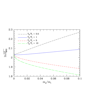
Figure 1: (Color) The BPS Coulomb logarithm $\ln\overline{\Lambda_{\rm\scriptscriptstyle BPS}^{\rm\scriptscriptstyle C}}$ plotted as a function of $m_{e}/m_{\rm\scriptscriptstyle I}$ for four values of the electron-ion temperature ratio, $T_{e}/T_{\rm\scriptscriptstyle I}=0.5\,,\,1,5\,,\,10$, all with the coupling $g_{e}=0.1$.

Adding Eq’s. (7) and (19), and comparing with the definition (2) of the Coulomb logarithm shows that in the classical limit

$$\ln\Lambda^{\rm\scriptscriptstyle C}_{\rm\scriptscriptstyle BPS} = {\sum}_{i}\,\frac{\omega_{i}^{2}}{\omega^{2}_{\rm\scriptscriptstyle I}}\,\left(1+\frac{T_{\rm\scriptscriptstyle I}m_{e}}{T_{e}m_{i}}\right)^{-3/2}\,\left(\,\ln\!\left\{\frac{4\,m_{ei}V^{2}_{ei}}{Z_{i}\,g_{e}\,T_{e}}\right\}-2\gamma\,\right)-\frac{1}{2}+\Delta\,.$$ (22)

This reduces to Eq. (5) in the limit $m_{e}\to 0$. Dimonte and Daligault dd use the conventional definition of the Coulomb logarithm for a single ion species rather than convention (2), one that applies to plasmas containing a variety of ions. For a single species of ions, the two conventions are related by

$$\ln\Lambda^{\!{\rm\scriptscriptstyle C}}=\left(1+\frac{T_{\rm\scriptscriptstyle I}m_{e}}{T_{e}m_{\rm\scriptscriptstyle I}}\,\right)^{-3/2}\,\ln\overline{\Lambda^{\!{\rm\scriptscriptstyle C}}}\,,$$ (23)

where we have denoted the conventional definition  of the Coulomb logarithm by $\ln\overline{\Lambda^{\rm\scriptscriptstyle C}}$. Pulling together previous definitions gives

$$\ln\overline{\Lambda^{\rm\scriptscriptstyle C}_{\rm\scriptscriptstyle BPS}} = \ln\!\left\{\frac{4}{Z_{\rm\scriptscriptstyle I}\,g_{e}}\right\}+\ln\!\left\{\frac{m_{\rm\scriptscriptstyle I}}{m_{\rm\scriptscriptstyle I}+m_{e}}\left(1+\frac{T_{\rm\scriptscriptstyle I}m_{e}}{T_{e}m_{\rm\scriptscriptstyle I}}\right)\right\}-2\gamma+\left(1+\frac{T_{\rm\scriptscriptstyle I}m_{e}}{T_{e}m_{I}}\right)^{3/2}\left[-\frac{1}{2}+\Delta\right]\ ,$$

which in Fig. 1 is plotted as a function of the electron-ion mass ratio for several values of the temperature ratio. Upon expanding to leading order in $m_{e}/m_{\rm\scriptscriptstyle I}$ we can express the Coulomb logarithm in terms of a zero electron-mass contribution and a correction,

$$\ln\overline{\Lambda^{\rm\scriptscriptstyle C}_{\rm\scriptscriptstyle BPS}} \simeq \ln\Lambda^{{\rm\scriptscriptstyle C}\,,\,{\rm\scriptscriptstyle 0}}_{\rm\scriptscriptstyle BPS}+\Delta\ln\!\overline{\Lambda_{\rm\scriptscriptstyle BPS}^{\rm\scriptscriptstyle C}}\ ,$$ (25)

where

$$\ln\Lambda^{{\rm\scriptscriptstyle C}\,,\,{\rm\scriptscriptstyle 0}}_{\rm\scriptscriptstyle BPS} = \ln\!\left\{\frac{4}{Z_{\rm\scriptscriptstyle I}\,g_{e}}\right\}-2\gamma-\frac{1}{2}$$ (26)

is the zero electron-mass limit, and

$$\Delta\ln\overline{\Lambda_{\rm\scriptscriptstyle BPS}^{\rm\scriptscriptstyle C}} = -\frac{m_{e}}{m_{\rm\scriptscriptstyle I}}\left(1-\frac{T_{\rm\scriptscriptstyle I}}{4T_{e}}\right)+\Delta$$ (27)

is the leading order electron mass correction. Dimonte and Daligault dd use $g_{e}=0.1$ and consider the cases in which $T_{e}/T_{\rm\scriptscriptstyle I}$ varies from about 1 to 5 with $m_{e}/m_{\rm\scriptscriptstyle I}$ varying from about zero to 0.02, while $Z_{\rm\scriptscriptstyle I}=1=n_{e}/n_{\rm\scriptscriptstyle I}$ are fixed. Figure 2 displays the values of $\Delta$ about this parameter range.

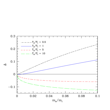
Figure 2: (Color) The correction $\Delta$ defined in Eq. (20) plotted as a function of the mass ratio $m_{e}/m_{\rm\scriptscriptstyle I}$ for a hydrogen plasma. The four curves correspond to the temperature ratios $T_{e}/T_{\rm\scriptscriptstyle I}=0.5,1,5,10$.

Figure 3 presents the complete leading corrections for the Coulomb logarithm (LABEL:firstcorr) as the mass ratio $m_{e}/m_{\rm\scriptscriptstyle I}$ is varied — Eq. (27) divided by Eq. (26). The leading term (26) is about 2.0, and so the relative correction is correspondingly smaller. Figure 3 shows that the relative size of the electron mass correction in the range examined by Dimonte and Daligault dd is less than 2%, which is less than their statistical accuracy of 5%. With smaller statistical error, one could resolve the mass effects (27) with an MD simulation.

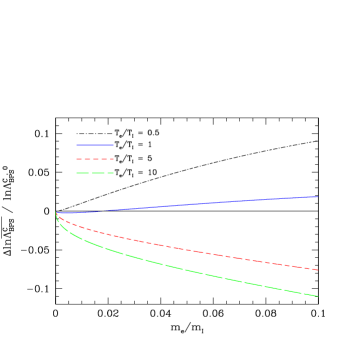
Figure 3: (Color) The relative electron-mass correction $\Delta\ln\overline{\Lambda_{\rm\scriptscriptstyle BPS}^{\rm\scriptscriptstyle C}}\,/\ln\Lambda_{\rm\scriptscriptstyle BPS}^{{\rm\scriptscriptstyle C}\,,\,{\rm\scriptscriptstyle 0}}$ plotted as a function of the mass ratio $m_{e}/m_{\rm\scriptscriptstyle I}$ for four values of the temperature ratio $T_{e}/T_{\rm\scriptscriptstyle I}=0.5,1,5,10$. In each case $g_{e}=0.1$. The mass correction $\Delta\ln\overline{\Lambda_{\rm\scriptscriptstyle BPS}^{\rm\scriptscriptstyle C}}$ is defined in Eq. (27), while the zero-mass logarithm $\ln\Lambda_{\rm\scriptscriptstyle BPS}^{{\rm\scriptscriptstyle C}\,,\,{\rm\scriptscriptstyle 0}}$ is given by Eq. (26).

Appendix A Results Collected

We put together here all the formulae relevant to the cases of physical interest in which the scattering is predominantly quantum mechanical. These include the small classical corrections to this purely quantum limit and the leading effects of Fermi-Dirac statistics that come into play as the electron density is increased. This we do because, with the inclusion of the $\Delta$ correction, we now have in hand all the small corrections to the leading quantum-mechanical scattering limit. To exhibit these, we write

$$\ln\Lambda_{{\rm\scriptscriptstyle BPS}}=\ln\Lambda^{\rm\scriptscriptstyle QM}_{{\rm\scriptscriptstyle BPS}}+\ln\Lambda^{{\rm\scriptscriptstyle\Delta C}}_{{\rm\scriptscriptstyle BPS}}+\ln\Lambda^{{\rm\scriptscriptstyle FD}}_{{\rm\scriptscriptstyle BPS}}\,.$$ (28)

Here $\ln\Lambda^{\rm\scriptscriptstyle QM}_{{\rm\scriptscriptstyle BPS}}$ is the leading term in the quantum limit together with the $\Delta$ correction that we have exhibited in the text, $\ln\Lambda^{{\rm\scriptscriptstyle\Delta C}}_{{\rm\scriptscriptstyle BPS}}$ is the first classical correction that appears when the parameters depart from the extreme quantum limit, and $\ln\Lambda^{{\rm\scriptscriptstyle FD}}_{{\rm\scriptscriptstyle BPS}}$ is the first correction when Fermi-Dirac statistics start to become important. The latter two terms have been computed in Ref. bs to leading order in the small ratio $m_{e}/m_{i}$; this suffices since the terms are already themselves small.

In the text we examined the limit of purely classical scattering and thus omitted the quantum correction term ${\cal C}^{{\rm\scriptscriptstyle\Delta Q}}_{e\,{\rm\scriptscriptstyle I}}$ in Eq. (6) from the complete relaxation rate. As a first step in presenting the collection mentioned, we quote this omitted correction which is Eq. (12.50) of BPS:

$${\cal C}^{\rm\scriptscriptstyle\Delta Q}_{e\,{\rm\scriptscriptstyle I}} \!\!=\! \!-{\sum}_{i}\frac{\kappa_{e}^{2}\,\kappa_{i}^{2}}{2}\,\frac{(T_{\rm\scriptscriptstyle I}^{2}m_{e}\,T_{e}^{2}m_{i})^{1/2}}{(T_{\rm\scriptscriptstyle I}m_{e}\!+\!T_{e}m_{i})^{3/2}}\!\left(\frac{1}{2\pi}\right)^{\!\!3/2}\!\!\int_{0}^{\infty}\!\!\!d\zeta\,e^{-\zeta/2}\left[{\rm Re}\,\,\psi\!\left\{\!1+i\frac{\bar{\eta}_{ei}}{\zeta^{1/2}}\right\}\!-\!\ln\!\left\{\frac{\bar{\eta}_{ei}}{\zeta^{1/2}}\right\}\right].$$

Here $\psi(z)=d\ln\Gamma(z)/dz$, and

$$\bar{\eta}_{ei}=\frac{|ee_{i}|}{\hbar V_{ei}}$$ (30)

makes precise the definition of the quantum parameter alluded to at the beginning of the text with the square of the thermal velocity in this expression $V_{ei}^{2}$ defined previously in Eq. (9). The extreme quantum limit in which $\bar{\eta}_{ei}\to 0$ of this formula is spelled out in detail in Ref. bps . Here we shall not repeat the derivation but simply quote the BPS limit (12.53) with slightly different notation:

$${\cal C}^{\rm\scriptscriptstyle\Delta Q}_{e\,{\rm\scriptscriptstyle I}} = {\sum}_{i}\frac{\kappa_{e}^{2}\,\kappa_{i}^{2}}{2}\,\frac{(T_{\rm\scriptscriptstyle I}^{2}m_{e}\,T_{e}^{2}m_{i})^{1/2}}{(T_{\rm\scriptscriptstyle I}m_{e}\!+\!T_{e}m_{i})^{3/2}}\!\left(\frac{1}{2\pi}\right)^{3/2}\,\left[3\gamma+\ln\!\left\{\frac{Z_{i}^{2}e^{4}}{2\hbar^{2}\,V_{ei}^{2}}\right\}\right]\,.$$ (31)

This quantum correction, added to the classical scattering contribution (7), produces

$${\cal C}^{\rm\scriptscriptstyle Q}_{e{\rm\scriptscriptstyle I},{\rm\scriptscriptstyle S}}={\sum}_{i}\frac{\kappa_{e}^{2}\,\kappa_{i}^{2}}{2}\,\frac{(T_{\rm\scriptscriptstyle I}^{2}m_{e}T_{e}^{2}m_{i})^{1/2}}{\left(T_{\rm\scriptscriptstyle I}m_{e}+T_{e}m_{i}\right)^{3/2}}\,\left(\frac{1}{2\pi}\right)^{3/2}\,\left[\ln\!\left\{\left(\frac{8\,T_{e}^{2}}{\hbar^{2}\omega_{e}^{2}}\right)\left(\frac{m^{2}_{ei}}{m_{e}}\frac{V^{2}_{ei}}{T_{e}}\right)\right\}-\gamma\,\right]\,.$$ (32)

In the same way that the classical Coulomb logarithm (22) was constructed, the quantum scattering version now reads

$$\ln\Lambda^{\rm\scriptscriptstyle QM}_{\rm\scriptscriptstyle BPS}={\sum}_{i}\,\frac{\omega_{i}^{2}}{2\omega_{\rm\scriptscriptstyle I}^{2}}\,\left(1+\frac{T_{\rm\scriptscriptstyle I}m_{e}}{T_{e}m_{i}}\right)^{-3/2}\,\left[\ln\!\left\{\left(\frac{8\,T_{e}^{2}}{\hbar^{2}\omega_{e}^{2}}\right)\left(\frac{m^{2}_{ei}}{m_{e}}\frac{V^{2}_{ei}}{T_{e}}\right)\right\}-\gamma\,\right]-\frac{1}{2}+\Delta\,.$$ (33)

The explicit electron-ions mass ratio terms that appear here (including those contained in the definition of $m_{ei}$ and $V^{2}_{ei}$ ) are easy to compute. For typical ICF conditions, they make very small corrections on the order or less than 1%. So as to make the significance of the $\Delta$ correction clear, a correction that does require some computation, we now omit these small explicit terms and write

$$\ln\Lambda^{\rm\scriptscriptstyle QM}_{\rm\scriptscriptstyle BPS}=\frac{1}{2}\,\left[\ln\!\left\{\frac{8\,T_{e}^{2}}{\hbar^{2}\omega_{e}^{2}}\right\}-\gamma-1\,\right]+\Delta\,,$$ (34)

which is precisely the result (4) of the text, but with the additional finite electron mass correction $\Delta$.

We show the $\Delta$ correction in Fig. 4 over a wide range of the temperature ratio $T_{\rm\scriptscriptstyle I}/T_{e}$ for the typical ICF case of an equimolar DT plasma. For a burning plasma, the Coulomb logarithm has the rough value $\ln\Lambda^{\rm\scriptscriptstyle QM}_{\rm\scriptscriptstyle BPS}\approx 4$, and so the relative $\Delta$ correction is about a quarter of the number shown in Fig. 4.

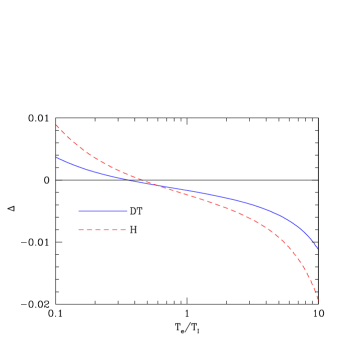
Figure 4: (Color) The correction $\Delta$ defined in Eq. (20) for an equimolar DT plasma (solid) and a hydrogen plasma (dashed) plotted as a function $T_{e}/T_{\rm\scriptscriptstyle I}$ for the physical values of the electron and ion masses.

For the remaining terms in Eq. (28), we shall just quote the result from Eq. (2.6) presented in Ref. bs , namely

$$\ln\Lambda^{{\rm\scriptscriptstyle\Delta C}}_{{\rm\scriptscriptstyle BPS}}=-\,\frac{\epsilon_{\rm\scriptscriptstyle H}}{T_{e}}\,{\sum}_{i}\,\frac{Z_{i}^{2}\,\omega_{i}^{2}}{\omega_{\rm\scriptscriptstyle I}^{2}}\,\left[\zeta(3)\left(\ln\!\left\{\frac{T_{e}}{Z_{i}^{2}\,\epsilon_{\rm\scriptscriptstyle H}}\right\}-\gamma\right)-2\,\zeta^{\prime}(3)\right]\,,$$ (35)

and 

$$\ln\Lambda^{{\rm\scriptscriptstyle FD}}_{{\rm\scriptscriptstyle BPS}}=\frac{n_{e}\lambda_{e}^{3}}{2}\,\left[-\left(1-\frac{1}{2^{3/2}}\right)\,\frac{1}{2}\left[\ln\!\left\{\frac{8T_{e}^{2}}{\hbar^{2}\omega_{e}^{2}}\right\}-\gamma-1\right]+\left(\frac{1}{2}\,\ln 2+\frac{1}{2^{5/2}}\right)\right]\,.$$ (36)

The ratio $\epsilon_{\rm\scriptscriptstyle H}/T_{e}$ describes the relative size of the first quantum to classical correction, where

$$\epsilon_{\rm\scriptscriptstyle H}=\,\frac{e^{4}\,m_{e}}{2\,\hbar^{2}}\simeq 13.6\,{\rm eV}$$ (37)

is the binding energy of the hydrogen atom. The numerical values of the zeta-function and its derivative are

$$\zeta(3)=\sum_{k=1}^{\infty}\,\frac{1}{k^{3}}=1.20205\cdots\,,$$ (38)

and

$$\zeta^{\prime}(3)=-\sum_{k=1}^{\infty}\,\frac{1}{k^{3}}\,\ln k=-0.19812\cdots\,.$$ (39)

The electron thermal wave length

$$\lambda_{e}=\hbar\left(\frac{2\pi}{m_{e}T_{e}}\right)^{1/2}$$ (40)

sets the scale at which quantum statistics comes into play, with $z_{e}=n_{e}\lambda_{e}^{3}/2$ the electron fugacity.

For some temperature and number density regimes of interest, the two corrections (35) and (36) become comparable in size bs .

References

(1)
L.S. Brown, D.L. Preston, and R.L. Singleton Jr.,
Phys. Rep. 410, 237 (2005), arXiv: physics/0501084.
See also R.L. Singleton Jr., BPS Explained I: Temperature
Relaxation in a Plasma, arXiv: 0706.2680;
BPS Explained II: Calculating the Equilibration Rate
in the Extreme Quantum Limit, arXiv: 0712.0639.
(2)
See for example,
J.P. Hansen and I.R. McDonald,
Phys. Rev. A 23, 2041 (1981);
Phys. Lett. 97A, 42 (1983);
M.S. Murillo and M.W.C. Dharma-Wardana,
Phys. Rev. Lett. 100, 205005 (2008),
arXiv:0712.1564;
J.N. Glosli, F.R. Graziani, R.M. More, M.S. Murillo, F.H. Steitz,
M.P. Surh, L.X. Benedict, S. Hau-Riege, A.B. Bangdon, and
R.A. London, Rev. E 78, 025401(R) (2008),
arXiv: 0802.4037.
(3)
G. Dimonte and J. Daligault,
Phys. Rev. Lett. 101, 135001 (2008).
(4)
W.H. Barkas, W. Birnbaum, and F.M. Smith,
Phys. Rev. 101, 778 (1956);
W.H. Barkas, N.J. Dyer, and H.H. Heckman,
Phys. Rev. Lett. 11, 26, 138(E) (1963).
(5)
L. Brown and R. Singleton,
Physical Review E 76, 066404, (2007),
arXiv:0707.2370.
(6)
T. Kihara and O. Aono,
Journ. Phys. Soc. Japan, 18, 837 (1963).