The Density Matrix Renormalization Group for Strongly Correlated Electron Systems: A Generic Implementation

Abstract

The purpose of this paper is (i) to present a generic and fully functional implementation of the density-matrix renormalization group (DMRG) algorithm, and (ii) to describe how to write additional strongly-correlated electron models and geometries by using templated classes. Besides considering general models and geometries, the code implements Hamiltonian symmetries in a generic way and parallelization over symmetry-related matrix blocks.

PROGRAM SUMMARY

Manuscript title: The Density Matrix Renormalization Group for Strongly Correlated Electron Systems: A Generic Implementation
Author: Gonzalo Alvarez
Program title: DMRG++
Licensing provisions: See file LICENSE.
Programming language: C++
Computer(s) for which the program has been designed: PC Operating system(s) for which the program has been designed: Any, tested on linux RAM required to execute with typical data: 1GB (256MB is enough to run included test)
Has the code been vectorised or parallelized?: Yes
Number of processors used: 1 to 8
Keywords: density-matrix renormalization group, dmrg, strongly correlated electrons, generic programming
PACS: 71.10.Fd 71.27.+a 78.67.Hc
CPC Library Classification: 23 Statistical Physics and Thermodynamics
External routines/libraries used: BLAS and LAPACK
Code Location: Computer Physics Communications
Development code location: http://www.ornl.gov/~gz1/dmrgPlusPlus/
Nature of problem: Strongly correlated electrons systems, display a broad range of important phenomena, and their study is a major area of research in condensed matter physics. In this context, model Hamiltonians are used to simulate the relevant interactions of a given compound, and the relevant degrees of freedom. These studies rely on the use of tight-binding lattice models that consider electron localization, where states on one site can be labeled by spin and orbital degrees of freedom. The calculation of properties from these Hamiltonians is a computational intensive problem, since the Hilbert space over which these Hamiltonians act grows exponentially with the number of sites on the lattice.
Solution method: The DMRG is a numerical variational technique to study quantum many body Hamiltonians. For one-dimensional and quasi one-dimensional systems, the DMRG is able to truncate, with bounded errors and in a general and efficient way, the underlying Hilbert space to a constant size, making the problem tractable.
Running time: The test program runs in 15 seconds.
References: re:white92

1 Introduction

In many materials of technological interest strong interactions between the electrons lead to collective behavior. These systems, referred to as strongly correlated electrons systems, display a broad range of important phenomenare:alvarez07 , and their study is a major area of research in condensed matter physics. In this context, model Hamiltonians are used to simulate the relevant interactions of a given compound, and the relevant degrees of freedom. These studies rely on the use of tight-binding lattice models that consider electron localization, where states on one site can be labeled by spin and orbital degrees of freedom. Examples of these models include the Hubbard modelre:hubbard63 , re:hubbard64b , the t-J model re:spalek77 , re:spalek07 and the spin 1/2 Heisenberg model, which can be considered the undoped limit of the t-J model.

Non-perturbative methods to solve these fairly rich and complicated models includere:dagotto94 (i) quantum Monte Carlo methods, and (ii) diagonalization methods. These two paths to solve the problem are more or less complementary. Quantum Monte Carlo methods, being formulated in Matsubara frequency, have difficulty obtaining real frequency properties of the model (such as the density-of-states), and sometimes suffer from the so-called “sign problem”re:troyer05 . On the other hand, diagonalization methods usually work efficiently only at zero or low temperature, due to the high computational cost of obtaining a full spectrum. Indeed, for exact diagonalization methods, the Hilbert space over which the problem is formulated –and hence the size of the Hamiltonian matrix to be diagonalized– grows exponentially with the size of the system.

In 1992, S. White re:white92 introduced the density-matrix renormalization group (DMRG) method. The DMRG is a numerical variational technique to study quantum many body Hamiltonians that could be classified as a diagonalization method. For one-dimensional and quasi one-dimensional systems, this method is able to truncate, with bounded errors and in a general and efficient way, the underlying Hilbert space to a constant size. A full discussion of the DMRG is beyond the scope of the present paper, and I will only present a brief procedural description of the method. Readers not familiar with the method are referred to the many published reviews re:schollwock05 , re:hallberg06 , re:rodriguez02 , and to the original paper re:white92 .

The present paper and accompanying code can be used in different ways. Physicists will be able to immediately use the flexible input file to run the code (see Section 7) for the Hubbard model with inhomogeneous couplings, Hubbard U values, and on-site potentials, as well as different symmetries, either on one-dimensional chains or on n-leg ladders. Readers with knowledge of DMRG will be able to understand the motivation for abstraction in the implementation of the algorithm (Section 2). Readers with knowledge of C++ will be able to understand the overall implementation of the DMRG algorithm (Section 3), and write additional models (Section 4.1) and geometries (Section 4.2) by following the interface provided. Two models are included as examples: the Hubbard model and the spin 1/2 Heisenberg model, and two geometries: the one-dimensional chain and the n-leg ladder. Readers interested in parallelization and performance issues (Section 4.3) will be able to write other concrete concurrency classes suited to their particular hardware requirements, following the code’s parallelization abstract interface. Finally, conclusions are presented in Section 5.

Other software projects, such as the ALPS projectre:albuquerque07 , also implement the DMRG algorithm within their own frameworks. However, this paper and DMRG++ emphasize generic programming, strongly correlated electron systems, detailed explanations, and few or no software dependencies.

The rest of this section is dedicated to a brief overview of the DMRG method, and to introduce some conventions and notation used throughout the paper. Let us define block to mean a finite set of sites. Let $C$ denote the states of a single site. This set is model dependent. For the Hubbard model it is given by: $C=\{e,\uparrow,\downarrow,(\uparrow,\downarrow)\}$, where $e$ is a formal element that denotes an empty state. For the t-J model it is given by $C=\{e,\uparrow,\downarrow\}$, and for the spin 1/2 Heisenberg model by $C=\{\uparrow,\downarrow\}$. A real-space-based Hilbert space $\mathcal{V}$ on a block $B$ and set $C$ is a Hilbert space with basis $B^{C}$. I will simply denote this as $\mathcal{V}(B)$ and assume that $C$ is implicit and fixed. A real-space-based Hilbert space can also be thought of as the external product space of $\#B$ Hilbert spaces on a site, one for each site in block $B$. We will consider general Hamiltonians that act on Hilbert spaces $\mathcal{V}$, as previously defined.

I give a procedural description of the DMRG method in the following. We start with an initial block $S$ (the initial system) and $E$ (the initial environment). Consider two sets of blocks $X$ and $Y$. We will be adding blocks from $X$ to $S$, one at a time, and from $Y$ to $E$, one at a time. Again, note that $X$ and $Y$ are sets of blocks whereas $S$ and $E$ are blocks. This is shown schematically in Fig. 1. All sites in $S$, $X$, $Y$ and $E$ are numbered as shown in the figure.

Figure 1: Labeling of blocks for the DMRG procedure. Blocks from vector of blocks X are added one at a time to block $S$ to form the system and blocks from vector of blocks Y are added one at a time to E to form the environment. Blocks are vectors of integers. The integers (numbers at the top of the figure) label all sites in a fixed and unique way.

Now we start a loop for the DMRG “infinite” algorithm by setting $step=0$ and $\mathcal{V}_{R}(S)\equiv\mathcal{V}(S)$ and $\mathcal{V}_{R}(E)\equiv\mathcal{V}(E)$.

The system is grown by adding the sites in $X_{step}$ to it, and let $S^{\prime}=S\cup X_{step}$, i.e. the $step$-th block of $X$ to $S$ is added to form the block $S^{\prime}$; likewise, let $E^{\prime}=E\cup Y_{step}$. Let us form the following product Hilbert spaces: $\mathcal{V}(S^{\prime})=\mathcal{V}_{R}(S)\otimes\mathcal{V}(X_{step})$ and $\mathcal{V}(E^{\prime})=\mathcal{V}_{R}(E)\otimes\mathcal{V}(Y_{step})$ and their union $\mathcal{V}(S^{\prime})\otimes\mathcal{V}(E^{\prime})$ which is disjoint.

Consider $\hat{H}_{S^{\prime}\cup E^{\prime}}$, the Hamiltonian operator, acting on $\mathcal{V}(S^{\prime})\otimes\mathcal{V}(E^{\prime})$. We diagonalize $\hat{H}_{S^{\prime}\cup E^{\prime}}$ (using Lanczos) to obtain its lowest eigenvector:

$$|\psi\rangle=\sum_{\alpha\in\mathcal{V}(S^{\prime}),\beta\in\mathcal{V}(E^{\prime})}\psi_{\alpha,\beta}|\alpha\rangle\otimes|\beta\rangle,$$ (1)

where $\{|\alpha\rangle\}$ is a basis of $\mathcal{V}(S^{\prime})$ and $\{|\beta\rangle\}$ is a basis of $\mathcal{V}(E^{\prime})$.

Let us define the density matrices for system:

$$(\hat{\rho}_{S})_{\alpha,\alpha^{\prime}}=\sum_{\beta\in\mathcal{V}(E^{\prime})}\psi_{\alpha^{\prime},\beta}^{*}\psi_{\alpha,\beta}$$ (2)

in $\mathcal{V}(S^{\prime})$, and environment:

$$(\hat{\rho}_{E})_{\beta,\beta^{\prime}}=\sum_{\alpha\in\mathcal{V}(S^{\prime})}\psi_{\alpha,\beta^{\prime}}^{*}\psi_{\alpha,\beta}$$ (3)

in $\mathcal{V}(E^{\prime})$. We then diagonalize $\hat{\rho}_{S}$, and obtain its eigenvalues and eigenvectors, $w^{S}_{\alpha,\alpha^{\prime}}$ in $\mathcal{V}(S^{\prime})$ ordered in decreasing eigenvalue order. We change basis for the operator $H^{S^{\prime}}$ (and other operators as necessary), as follows:

$$(H^{S^{\prime}{\rm new\,\,basis}})_{\alpha,\alpha^{\prime}}=(w^{S})^{-1}_{\alpha,\gamma}(H^{S^{\prime}})_{\gamma,\gamma^{\prime}}w^{S}_{\gamma^{\prime},\alpha^{\prime}}.$$ (4)

We proceed in the same way for the environment, diagonalize $\hat{\rho}_{E}$ to obtain ordered eigenvectors $w^{E}$, and define $(H^{E^{\prime}{\rm new\,\,basis}})_{\alpha,\alpha^{\prime}}$.

Let $m_{S}$ be a fixed number that corresponds to the number of states in $\mathcal{V}(S^{\prime})$ that we want to keep. Consider the first $m_{S}$ eigenvectors $w^{S}$, and let us call the Hilbert space spanned by them, $\mathcal{V}_{R}(S^{\prime})$, the DMRG-reduced Hilbert space on block $S^{\prime}$. If $m_{S}\geq\#\mathcal{V}(S^{\prime})$ then we keep all eigenvectors and there is effectively no truncation. We truncate the matrices $(H^{S^{\prime}{\rm new\,\,basis}})$ (and other operators as necessary) such that they now act on this truncated Hilbert space, $\mathcal{V}_{R}(S^{\prime})$. We proceed in the same manner for the environment.

Now we increase $step$ by 1, set $S\leftarrow S^{\prime}$, $\mathcal{V}_{R}(S)\leftarrow\mathcal{V}_{R}(S^{\prime})$, $H_{S^{\prime}}\leftarrow H_{S}$, and similarly for the environment, and continue with the growth phase of the algorithm.

In the infinite algorithm, the number of sites in the system and environment grows as more steps are performed. After this infinite algorithm, a finite algorithm is applied where the environment is shrunk at the expense of the system, and the system is grown at the expense of the environment. During the finite algorithm phase the total number of sites remains constant allowing for a formulation of DMRG as a variational method in a basis of matrix product states. The advantage of the DMRG algorithm is that the truncation procedure described above keeps the error bounded and small. Assume $m_{S}=m_{E}=m$. At each DMRG stepre:dechiara08 the truncation error $\epsilon_{tr}=\sum_{i>m}\lambda_{i}$, where $\lambda_{i}$ are the eigenvalues of the truncated density matrix $\rho_{S}$ in decreasing order. The parameter $m$ should be chosen such that $\epsilon_{tr}$ remains small, say re:dechiara08 $\epsilon_{tr}<10^{-6}$. For critical 1D systems $\epsilon_{tr}$ decays as a function of $m$ with a power law, while for 1D system away from criticality it decays exponentially. For a more detailed description of the error introduced by the DMRG truncation in other systems see re:dechiara08 , re:schollwock05 , re:hallberg06 , re:rodriguez02 .

2 Motivation for Generic Programming

Let us motivate the discussion by introducing a typical problem to be solved by DMRG: “Using the DMRG method, one would like to calculate the local density of states on all sites for a Hubbard model with inhomogeneous Hubbard U values on a one-dimensional (1D) chain”. We want to modularize as many tasks mentioned in the last sentence as possible. We certainly want to separate the DMRG solver from the model in question, since we could later want to do the same calculation for the t-J model; and the model from the lattice, since we might want to do the same calculation on, say, a n-leg ladder, instead of a 1D chain. C++ is a computer language that is very fit for this purpose, since it allows to template classes. Then we can write a C++ class to implement the DMRG method (DmrgSolver class), and template this class on a strongly-correlated-electron (SCE) model template, so that we can delegate all SCE model related code to the SCE model class.

However, for DmrgSolver to be able to use a given SCE model, we need a convention that such SCE model class will have to follow. This is known as a C++ public interface, and for a SCE model it is given in DmrgModelBase. To do the calculation for a new SCE model, we simply need to implement all functions found in DmrgModelBase without changing the DmrgSolver class. The model will, in turn, be templated on the geometry. For example, the Hubbard model with inhomogeneous Hubbard U values and inhomogeneous hoppings (class DmrgModelHubbard) delegates all geometry related operations to a templated geometry class. Then DmrgModelHubbard can be used for, say, one-dimensional chains and n-leg ladders without modification. This is done by just instantiating DmrgModelHubbard with the appropriate geometry class, either DmrgGeometryOneD or DmrgGeometryLadder, or some other class that the reader may wish to write, which implements the interface given in DmrgGeometryBase.

In the following sections I will describe these different modules. Since the reader may wish to first understand how the DMRG method is implemented, I will start with the core C++ classes that implement the method. The user of the program will not need to change these core classes to add functionality. Instead, new models and geometries can be added by creating implementations for DmrgModelBase and DmrgGeometryBase, and those public interfaces will be explained next.

But for now I end this section by briefly describing the “driver” program for a Hubbard model on a 1D chain. The driver program is contained in the file main.cpp. This file is created by the configure.pl script after answering questions related to model and geometry (see also Section 7). There, DmrgSolver is instantiated with DmrgModelHubbard, since in this case one wishes to perform the calculation for the Hubbard model. In turn, DmrgModelHubbard is instantiated with DmrgGeometryOneD since now one wishes to perform the calculation on a 1D chain.

3 Core Classes: The DMRG Solver and Bases

3.1 DmrgSolver and The “Infinite” DMRG Algorithm

The purpose of the DmrgSolver class is to perform the loop for the DMRG “infinite algorithm” discussed before. This class also performs the “finite algorithm” re:schollwock05 to allow for the calculation of observables, such as the local density of states of the cluster, defined as

$$N_{i}(\omega)=\int_{-\infty}^{\infty}\,dt\,\langle\psi|e^{-i\hat{H}t}c^{\dagger}_{i}e^{i\hat{H}t}c_{i}\,e^{i\omega t}|\psi\rangle,$$ (5)

where $|\psi\rangle$ is the ground state of the system. The program is structured as a series of header files containing the implementation with each class written in the header file of the same name, and a “driver” program that uses the capabilities provided by the header files to solve a specific problem. To simplify the discussion, we start where the “driver program” starts, in its int main() function, which calls dmrgSolver.main(), whose main work is to perform the loop for the “infinite” DMRG algorithm. Let us now discuss this loop which is found in the infiniteDmrgLoop function, and is sketched in Fig. 2.

⬇

for (step=0;step<X.size();step++) {

// grow system (a)

grow(pSprime,pS,X[step],model,GROW_RIGHT);

// grow environment (b)

grow(pEprime,pE,Y[step],model,GROW_LEFT;

// product of system and environment (c)

pSE.setToProduct(pSprime,pEprime);

diagonalize(psi,pSprime,pEprime,pSE,

model); // (d)

ns=pSprime.size();

ne=pEprime.size();

changeAndTruncateBasis(pS,psi,pSprime,ns,ne,

pSE,0); // (e)

changeAndTruncateBasis(pE,psi,pEprime,ns,ne,

pSE,1); // (f)

systemStack.push(pS); //(g)

}

Figure 2: Implementation of the “infinite” DMRG loop for a general SCE model on a general geometry.

In Fig. 2(a) the system pS is grown by adding the sites contained in block X[step]. Note that X is a vector of blocks to be added one at a time. The block X[step] (usually just a single site) is added to the right of pS, hence the GROW_RIGHT flag. The result is stored in pSprime. Similarly is done in Fig. 2(b) for the environment: the block Y[step] (usually just a single site) is added to the environment given in pE and stored in pEprime. This time the addition is done to the left of pE, since pE is the environment. In Fig. 2(c) the outer product of pSprime (the new system) and pEprime (the new environment) is made and stored in pSE. The actual task is delegated to the DmrgBasis class (see Section 3.2). In Fig. 2(d) the diagonalization of the Hamiltonian for block pSE is performed, and the ground state vector is computed and stored in psi, following Eq. (1). Next, in Fig. 2(e) the bases are changed following Eqs. (2,3,4), truncated if necessary, and the result is stored in pS for the system, and in pE, Fig. 2(f), for the environment. Note that this overwrites the old pS and pE, preparing these variable for the next DMRG step.

A copy of the current state of the system is pushed into a last-in-first-out stack in Fig. 2(g), so that it can later be used in the finite DMRG algorithm (not discussed here, see code). The loop continues until all blocks in vector of blocks X have been added to the initial system S, and all blocks in vector of blocks Y have been added to the initial environment E. We repeat again that vector of sites are used instead of simply sites to generalize the growth process, in case one might want to add more than one site at a time.

I will later go back to this infinite DMRG loop and discuss the implementation of the steps mentioned in the previous paragraph (i.e., growth process, outer products, diagonalization, change of basis and truncation). However, some of these capabilities need first the introduction of two new C++ classes to handle operations related to Hilbert space bases.

3.2 DmrgBasis Class: Implementation of Symmetries

DMRG++ has two C++ classes that handle the concept of a basis (of a Hilbert space). The first one (DmrgBasis) handles reordering and symmetries in a general way, without the need to consider operators. The second one (DmrgBasisWithOperators) does consider operators, and will be explained in the next sub-section. The advantage of dividing functionality in this way will become apparent later.

In any actual computer simulation the “infinite” DMRG loop will actually stop at a certain point. Let us say that it stops after 50 sites have been added to the system. There will also be at this point another 50 sites that constitute the environment. Now, from the beginning each of these 100 sites is given a fixed number from 0 to 99. Therefore, sites are always labeled in a fixed way and their labels are always known (see Fig. 1). The variable block_ of a DmrgBasis object indicates over which sites the basis represented by this object is being built. To explain the rest of the capability handled by the DmrgBasis class, I need to explain how symmetries are treated in the program, and how the Hilbert space basis is partitioned. This is explained in the following.

Symmetries will allow the solver to block the Hamiltonian matrix in blocks, using less memory, speeding up the computation and allowing the code to parallelize matrix blocks related by symmetry. Let us assume that our particular model has $N_{s}$ symmetries labeled by $0\leq\alpha<N_{s}$. Therefore, each element $k$ of the basis has $N_{s}$ associated “good” quantum numbers $\tilde{q}_{k,\alpha}$. These quantum numbers can refer to practically anything, e.g., to number of particles with a given spin or orbital or to the $z$ component of the spin. We do not need to know the details to block the matrix. However, we know that these numbers are finite, and let $Q$ be an integer such that $\tilde{q}_{k,\alpha}<Q$ $\forall k,\alpha$. We can then combine all these quantum numbers into a single one, like this: $q_{k}=\sum_{\alpha}\tilde{q}_{k,\alpha}Q^{\alpha}$, and this mapping is bijective. In essence, we combined all “good” quantum numbers into a single one and from now on we will consider that we have only one Hamiltonian symmetry called the “effective” symmetry, and only one corresponding number $q_{k}$, the “effective” quantum number. These numbers are stored in the member quantumNumbers of C++ class DmrgBasisImplementation. (Note that if one has 100 sites or less, then the number $Q$ defined above is probably of the order of hundreds for usual symmetries, making this implementation very practical for systems of correlated electrons.)

We then reorder our basis such that its elements are given in increasing $q$ number. There will be a permutation vector associated with this reordering, that will be stored in the member permutationVector of class DmrgBasisImplementation.

What remains to be done is to find a partition of the basis which labels where the quantum number changes. Let us say that the quantum numbers of the reordered basis states are $\{3,3,3,3,8,8,9,9,9,15,\cdots\}$. Then we define a vector named “partition”, such that partition[0]=0, partition[1]=4, because the quantum number changes in the 4th position (from 3 to 8), and then partition[2]=6, because the quantum number changes again (from 8 to 9) in the 6th position, etc. Now we know that our Hamiltonian matrix will be composed first of a block of 4x4, then of a block of 2x2, etc.

The quantum numbers of the original (untransformed) real-space basis are set by the model class (to be described in Section 4.1), whereas the quantum numbers of outer products are handled by the class DmrgBasis. This can be done because if $|a\rangle$ has quantum number $q_{a}$ and $|b\rangle$ has quantum number $q_{b}$, then $|a\rangle\otimes|b\rangle$ has quantum number $q_{a}+q_{b}$. DmrgBasis also knows how quantum numbers change when we change the basis: they do not change since the DMRG transformation preserves quantum numbers; and DmrgBasis also knows what happens to quantum numbers when we truncate the basis: quantum numbers of discarded states are discarded. In this way, symmetries are implemented efficiently, with minimal dependencies and in a model-independent way.

3.3 DmrgBasisWithOperators Class and Outer Product of Operators

C++ class DmrgBasis implements only certain functionality associated with a Hilbert space basis, as mentioned in the previous section. However, more capabilities related to a Hilbert space basis are needed.

C++ class DmrgBasisWithOperators inherits from DmrgBasis, and contains certain local operators for the basis in question, as well as the Hamiltonian matrix. The operators that need to be considered here are operators necessary to compute the Hamiltonian across the system and environment, and to compute observables. Therefore, the specific operators vary from model to model. For example, for the Hubbard model, we consider $c_{i\sigma}$ operators, that destroy an electron with spin $\sigma$ on site $i$. For the spin 1/2 Heisenberg model, we consider operators $S^{+}_{i}$ and $S^{z}_{i}$ for each site $i$. In each case these operators are calculated by the model class (see Section 4.1) on the “natural” basis, and added to the basis in question with a call to setOperators(). These local operators are stored as sparse matrices to save memory, although the matrix type is templated and could be anything. For details on the implementation of these operators, see OperatorsBase and the two examples provided OperatorsHubbard and OperatorsHeisenberg for the Hubbard and Heisenberg models, respectively. Additionally, DmrgBasisWithOperators has a number of member functions to handle operations that the DMRG method performs on local operators in a Hilbert space basis. These include functions to create an outer product of two given Hilbert spaces, to transform a basis, to truncate a basis, etc.

Let us now go back to the “infinite” DMRG loop and discuss in more detail Fig. 2(a) ((b) is similar)), i.e., the function grow(), which is found in DmrgSolver. Local operators are set for the basis in question with a call to DmrgBasisWithOperators’s member function setOperators(). When adding sites to the system or environment the program does a full outer product, i.e., it increases the size of all local operators. This is performed by the call to setToProduct(pSprime,pS,Xbasis,dir,option) in the grow function, which actually calls pSprime.setToProduct(pS,xBasis,dir). This function also recalculates the Hamiltonian in the outer product of (i) the previous system basis $pS$, and (ii) the basis $Xbasis$ corresponding to the site(s) that is (are) being added. To do this, the Hamiltonian connection between the two parts needs to be calculated and added, and this is done in the call to addHamiltonianConnection, found in the function grow(). Finally, the resulting dmrgBasis object for the outer product, pSprime, is set to contain this full Hamiltonian with the call to pSprime.setHamiltonian(matrix).

I will now explain how the full outer product between two operators is implemented. If local operator $A$ lives in Hilbert space $\mathcal{A}$ and local operator $B$ lives in Hilbert space $\mathcal{B}$, then $C=AB$ lives in Hilbert space $\mathcal{C}=\mathcal{A}\otimes\mathcal{B}$. Let $\alpha_{1}$ and $\alpha_{2}$ represent states of $\mathcal{A}$, and let $\beta_{1}$ and $\beta_{2}$ represent states of $\mathcal{B}$. Then, in the product basis, $C_{\alpha_{1},\beta_{1};\alpha_{2},\beta_{2}}=A_{\alpha_{1},\alpha_{2}}B_{\beta_{1},\beta_{2}}$. Additionally, $\mathcal{C}$ is reordered such that each state of this outer product basis is labeled in increasing effective quantum number (see Section 3.2). In the previous example, if the Hilbert spaces $\mathcal{A}$ and $\mathcal{B}$ had sizes $a$ and $b$, respectively, then their outer product would have size $ab$. When we add sites to the system (or the environment) the memory usage remains bounded by the truncation, and it is usually not a problem to store full product matrices, as long as we do it in a sparse way (DMRG++ uses compressed row storage). In short, local operators are always stored in the most recently transformed basis for all sites and, if applicable, all values of the internal degree of freedom $\sigma$.

This simplifies the implementation, but it must be remembered that only the local operators corresponding to the most recently added sites will be meaningful. Indeed, if we apply transformation $W$ (possibly truncating the basis, see Eq. (4)) then

$$(W^{\dagger}AW)(W^{\dagger}BW)\neq W^{\dagger}(AB)W,$$ (6)

since $WW^{\dagger}\neq 1$ because the DMRG truncation does not assure us that $W^{\dagger}$ will be the right inverse of $W$ (but $W^{\dagger}W=1$ always holds). Because of this reason we cannot construct the Hamiltonian simply from transformed local operators, even if we store them for all sites, but we need to store also the Hamiltonian in the most recently transformed basis. The fact that DmrgBasisWithOperators stores local operators in the most recently transformed basis for all sites does not increase memory usage too much, and simplifies the writing of code for complicated geometries or connections. The SCE model class is responsible for determining whether a transformed operator can be used (or not because of the reason mentioned above).

Let us now examine in more detail Fig. 2(c), where we form the outer product of the current system and current environment, and calculate its Hamiltonian. We could use the same procedure as outlined in the previous paragraph, i.e., to use the DmrgBasisWithOperators class to resize the matrices for all local operators. Storing matrices in this case (even in a sparse way and even considering that there is truncation) would be too much of a penalty for performance. Therefore, in this latter case we do the outer product on-the-fly only, without storing any matrices. In Fig. 2(c) pSE contains the outer product of system and environment, but pSE is only a DmrgBasis object, not a DmrgBasisWithOperators object, i.e., it does not contain operators.

We now consider Fig. 2(d), where the diagonalization of the system’s plus environment’s Hamiltonian is performed. Since pSE, being only a DmrgBasis object, does not contain all the information related to the outer product of system and environment (as we saw, this would be prohibitively expensive), we need to pass the system’s basis (pSprime) and the environment’s basis (pEprime) to the diagonalization function (diagonalize() in DmrgSolver) in order to be able to form the outer product on-the-fly. There, since pSE does provide information about effective symmetry blocking, we block the Hamiltonian matrix using effective symmetry, and call diagonaliseOneBlock() in DmrgSolver for each symmetry block. Only those matrix blocks that contain the desired or targeted number of electrons will be considered. To diagonalize Hamiltonian H we use the Lanczos methodre:lanczos50 , re:pettifor85 , although this is also templated.

For the Lanczos diagonalization method we also want to provide as much code isolation and modularity as possible. The Lanczos method needs only to know how to perform the operation $x$ += H$y$, given vectors $x$ and $y$. Using this fact, we can separate the matrix type from the Lanczos method. To keep the discussion short this is not addressed here, but can be seen in the diagonaliseOneBlock() function, and in classes SolverLanczos, HamiltonianInternalProduct, and DmrgModelHelper. The first of these classes contains an implementation of the Lanczos method that is templated on a class that simply has to provide the operation $x$ += H$y$ and, therefore, it is generic and valid for any SCE model. It is important to remark that the operation $x$ += H$y$ is finally delegated to the model in question. As an example, the operation x += H for the Hubbard model is performed in function matrixVectorProduct() in class DmrgModelHubbard. This function performs only three tasks: (i) $x$ += H${}_{system}y$, (ii) $x$ += H${}_{environment}y$ and (iii) $x$ += H${}_{connection}y$. The fist two are straightforward, so we focus on the last one, in hamiltonianConnectionProduct(), that considers the part of the Hamiltonian that connects system and environment. This function runs the following loop: for every site $i$ in the system and every site $j$ in the environment it calculates $x$ += H${}_{ij}y$ in function linkProduct, after finding the appropriate tight binding hopping value.

The function linkProduct is useful not only for the Hubbard model, but it is generic enough to use in other SCE models that include a tight binding connection of the type $c^{\dagger}_{i\sigma}c_{j\sigma}$, and, therefore, is part of a separate class, ConnectorHopping. Likewise, the function linkProduct in ConnectorExchange deals with Hamiltonian connections of the type $\vec{S}_{i}\cdot\vec{S}_{j}$, and can be used by models that include that type of term, such as the sample spin 1/2 Heisenberg model provided with DMRG++. We remind readers that wish to understand this code that the function linkProduct and, in particular, the related function fastOpProdInter are more complicated than usual, since (i) the outer product is constructed on the fly, and (ii) the resulting states of this outer product need to be reordered so that effective symmetry blocking can be used.

4 Abstract Classes

4.1 The Model Interface

A sample SCE model, the one-band Hubbard model,

$$\sum_{i,j,\sigma}t_{ij}c^{\dagger}_{i\sigma}c_{j\sigma}+\sum_{i}U_{i}n_{i\uparrow}n_{i\downarrow}+\sum_{i,\sigma}V_{i}n_{i\sigma},$$

is implemented in class DmrgModelHubbard. A sample DmrgModelHeisenberg is also included for the spin 1/2 Heisenberg model $\sum_{ij}J_{ij}\vec{S}_{i}\cdot\vec{S}_{j}$. These models inherit from the abstract class DmrgModelBase. To implement other SCE models one has to implement the functions prototyped in that abstract class. The interface (functions in DmrgModelBase) are documented in place; here I briefly describe some of them. The matrixVectorProduct function needs to implement the operation $x$ += H$y$. The function addHamiltonianConnection implements the Hamiltonian connection (e.g. tight-binding links in the case of the Hubbard Model or products $S_{i}\cdot S_{j}$ in the case of the spin 1/2 Heisenberg model) between two basis, $basis2$ and $basis3$, in the order of the outer product, $basis1={\rm SymmetryOrdering}(basis2\otimes basis3)$. This was explained before in Section 3.3, and the examples shown by DmrgModelHubbard and DmrgModelHeisenberg will be helpful in the implementation of other models. Function setNaturalBasis sets certain aspects of the “natural basis” (usually the real-space basis) on a given block. The operator matrices (e.g., $c^{\dagger}_{i\sigma}$ for the Hubbard model or $S_{i}^{+}$ and $S_{i}^{z}$ for the spin 1/2 Heisenberg model) need to be set there, as well as the Hamiltonian and the effective quantum number for each state of this natural basis. To implement the algorithm for a fixed density, the number of electrons for each state is also needed .

4.2 The Geometry Interface

I present two sample geometries, one for 1D chains and one for n-leg ladders in classes DmrgGeometryOneD and DmrgGeometryLadder. Both derive from the abstract class DmrgGeometryBase. To implement new geometries a new class needs to be derived from this base class, and the functions in the base class (the interface) needs to be implemented. As in the case of DmrgModelBase, the interface is documented in the code, but here I briefly describe the most important functions.

The function setBlocksOfSites needs to set the initial block for system and environment, and for the vector of blocks $X$ and $Y$ to be added to system and environment, respectively, according to the convention given in Fig. 1. There are two calcConnectorType functions. Both calculate the type of connection between two sites $i$ and $j$, which can be SystemSystem, SystemEnviron, EnvironSystem or EnvironEnviron, where the names are self-explanatory. The function calcConnectorValue determines the value of the connector (e.g., tight-binding hopping for the Hubbard model or $J_{ij}$ for the case of the spin 1/2 Heisenberg model) between two sites, delegating the work to the model class if necessary. The function findExtremes determines the extremes sites of a given block of sites and the function findReflection finds the “reflection” in the environment block of a given site in the system block or vice-versa.

4.3 The Concurrency Interface: Code Parallelization

The Concurrency class encapsulates parallelization. Two concrete classes that implement this interface are included in the present code. One is for serial code (ConcurrencySerial class) that does no parallelization at all, and the other one (ConcurrencyMpi class) is for parallelization based on the MPI. Other parallelization implementations, e.g. using pthreads, can be similarly written by implementing this interface. The interface is described in place in class Concurrency. Here, I briefly mention its most important functions. Function rank() returns the rank of the current processor or thread. nprocs() returns the total number of processors. Functions loopCreate() and loop() handle a parallelization of a standard loop. Function gather() gathers data from each processor into the root processor.

5 Conclusions

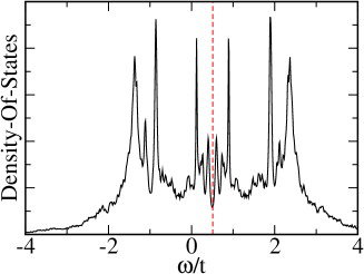
Figure 3: Ground-State Density-Of-States of the Hubbard Model on a 32 site chain with a constant Hubbard $U=1.0$ and density 1.0.

This paper presents DMRG++, a code to calculate properties of strongly correlated electron models with the DMRG method. The paper explains how to use the code for the Hubbard and spin 1/2 Heisenberg models on a one dimensional chain and on n-leg ladders, and how to add new models and geometries through the use of public interfaces. The rationale behind the design of the generic DMRG algorithm is also explained, as well as the implications for memory usage and performance. The ideas used in the code –and explained in the paper– regarding symmetry blocking, treatment of Hamiltonian connections and parallelization, can be of inspiration to other researchers. The code implements two efficiency techniques (suggested originally in re:white96 ): (i) the wave function transformation which transforms the wave function from the previous step to the current step to use as the initial vector for the Lanczos solver, and (ii) the use of different truncation values “m” for different finite size loops. Other efficiency improvements will be added to the present code in the future, for example, the use of “disk stacks” instead of memory stacks (std::stack will be replaced by a DiskStack class), and the implementation of the reflection symmetry for the infinite size algorithm (implying a factor of 2 gain during the infinite size algorithm phase). Future work will also include a systematic treatment of “correlation” observables of the type $\langle\hat{O}_{i}\hat{O}_{j}\rangle$, which can be addressed in a generic way.

6 Acknowledgments

The present code uses part of the psimag toolkit, http://psimag.org/. Thomas Schulthess and Michael Summers’s work on psimag has inspired some of the C++ templated classes used in DMRG++. I would like to thank Jose Riera and Ivan Gonzalez for helping me with the validation of results and extensive tests for the DMRG code on chains and ladders. I acknowledge the support of the Center for Nanophase Materials Sciences, sponsored by the Scientific User Facilities Division, Basic Energy Sciences, U.S. Department of Energy, under contract with UT-Battelle.

7 Test Run

1. Download source code from here http://www.ornl.gov/~gz1/dmrgPlusPlus/ (a stable version will be published by Computer Physics Communications)

2. Create a sample driver code (main.cpp file) for the program by executing:
   perl configure.pl
   and answering the questions regarding model and geometry. Defaults values can be chosen by pressing enter. This will also create a Makefile and sample input file.

3. Run make to compile and link the code. The LAPACK library is required by the program. File INSTALL contains more details on compilation.

4. Optionally, edit the sample input input.inp to adjust the parameters of the run. This file is self-explanatory.

5. Run the code with ./dmrg input.inp > output.dat

6. Note1: Progress is written to standard output. Energies and continued-fraction data is written to the file specified in input.inp:

   parameters.numberOfKeptStates=64
   parameters.linSize=8
   parameters.density=1
   ...
   (other echo of input omitted)
   #Energy=-3.57537
   #Energy=-5.62889
   #Energy=-7.69483
   #Energy=-9.76627
   ...
   

7. Note2: To obtain local density of states data (such as Fig. 3): (i) run the code with the option calculateLDOS (see file README for a description of the options line in the input file) and (ii) process the continued fraction data as follows:

   perl contfraction.pl data.txt 16 -4 4 0.01 > figure.dos
   

   where [-4,4] is the energy interval over which the local density of states calculation is to be performed and 0.01 is the energy step increment. The method used to compute the density of states data is the continued-fraction method re:hallberg95 . Other methods, such as the correction vector methodre:kuhner99 , have been proposed (see re:hallberg06 for a detailed review).

8. Note3: A detailed explanation of compilation instructions and required software can be found in the file INSTALL. A detailed explanation of input and output can be found in the file README.

References

- [1] White, S., Phys. Rev. Lett. 69 (1992) 2863.
- [2] Alvarez, G. et al., J. Phys.: Condens. Matter 19 (2007) 125213.
- [3] Hubbard, J., Proc. R. Soc. London Ser. A 276 (1963) 238.
- [4] Hubbard, J., Proc. R. Soc. London Ser. A 281 (1964) 401.
- [5] Spalek, J. and Oleś, A., Physica B 86-88 (1977) 375.
- [6] Spalek, J., Acta Physica Polonica A 111 (2007) 409.
- [7] Dagotto, E., Review of Modern Physics 66 (1994) 763.
- [8] Troyer, M. and Wiese, U.-J., Phys. Rev. Lett. 94 (2005) 170201.
- [9] Schollwöck, U., Rev. Mod. Phys. 77 (2005) 259.
- [10] Hallberg, K., Adv. Phys. 55 (2006) 477.
- [11] Rodriguez-Laguna, J., http://arxiv.org/abs/cond-mat/0207340, Real Space Renormalization Group Techniques and Applications, 2002.
- [12] F. Albuquerque et al. (ALPS collaboration), Journal of Magnetism and Magnetic Materials 310 (2007) 1187.
- [13] Chiara, G. D., Rizzi, M., Rossini, D., and Montangero, S., J. Comput. Theor. Nanosci. 5 (2008) 1277.
- [14] Lanczos, C., J. Res. Nat. Bur. Stand. 45 (1950) 255.
- [15] Pettifor, D. and Weaire, D., editors, The Recursion Method and Its Applications, Springer Series in Solid-State Sciences, volume 58, Springer Verlag, Berlin/Heidelberg, 1985.
- [16] White, S., Phys. Rev. Lett. 77 (1996) 3633.
- [17] Hallberg, K., Phys. Rev. B 52 (1995) 9827.
- [18] Kühner, T. and White, S., Phys. Rev. B 60 (1999) 335.