The gravitational wave background from star-massive black hole fly-bys

Abstract

Stars on eccentric orbits around a massive black hole (MBH) emit bursts of gravitational waves (GWs) at periapse. Such events may be directly resolvable in the Galactic centre. However, if the star does not spiral in, the emitted GWs are not resolvable for extra-galactic MBHs, but constitute a source of background noise. We estimate the power spectrum of this extreme mass ratio burst background (EMBB) and compare it to the anticipated instrumental noise of the Laser Interferometer Space Antenna (LISA). To this end, we model the regions close to a MBH, accounting for mass-segregation, and for processes that limit the presence of stars close to the MBH, such as GW inspiral and hydrodynamical collisions between stars. We find that the EMBB is dominated by GW bursts from stellar mass black holes, and the magnitude of the noise spectrum $(fS_{\rm GW})^{1/2}$ is at least a factor $\sim 10$ smaller than the instrumental noise. As an additional result of our analysis, we show that LISA is unlikely to detect relativistic bursts in the Galactic centre.

1 Introduction

A new opportunity to study stellar processes near massive black holes (MBHs) arises with the anticipated detection of gravitational waves (GWs) by the Laser Interferometer Space Antenna (LISA). LISA will be a space-based detector in orbit around the Sun, consisting of three satellites five million kilometres apart. It will be sensitive to GWs in a frequency range $10^{-4}{\,\rm Hz}\lesssim f\lesssim 10^{-2}$ Hz. An important source of GWs for LISA is the inspiral of compact objects onto MBHs in galactic nuclei (e.g. Hils & Bender 1995; Sigurdsson & Rees 1997; Ivanov 2002; Freitag 2003; Hopman & Alexander 2005, 2006a, 2006b; Amaro-Seoane et al. 2007; see Hopman 2006 for a review). These are sources on highly eccentric orbits with periapses slightly larger than the Schwarzschild radius $r_{S}=2GM_{\bullet}/c^{2}$ of the MBH, where $M_{\bullet}$ is the mass of the MBH. The star dissipates energy due to GW emission, and as a result spirals in. Such extreme mass ratio inspirals (EMRIs) can be observed by LISA to cosmological distances if the orbital period of the star is shorter than $P\lesssim 10^{4}$ sec (Finn & Thorne 2000; Barack & Cutler 2004; Gair et al. 2004; Glampedakis 2005). LISA will detect hundreds to thousands of such captures over its projected 3-5 yr mission life time (Gair et al., 2004; Gair, 2008).

For most of the inspiral the emitted GWs are not observable by LISA. These GWs give rise to a source of confusion noise, possibly obscuring other types of GW sources. The shape and overall magnitude of this EMRI background has been studied by Barack & Cutler (2004). They do not study the dynamical requirements of inspiral, but scale their result with possible EMRI rates of Freitag (2001, 2003). Therefore noise of stars that do not eventually spiral in is not included.

Rubbo et al. (2006) show that stars on long periods of a few years and nearly radial orbits that carry them near the Schwarzschild radius of the MBH, emit bursts of GWs that for the Galactic centre will give a signal to noise ratio larger than 5. Taking into account processes determining the inner radius of the density profile as well as mass segregation effects, Hopman et al. (2007) find that stellar mass black holes (BHs) have a burst rate of order $1$ yr^-1, while the rate is $\lesssim 0.1$ yr^-1 for main sequence stars (MSs) and white dwarfs (WDs).

Individual bursts from star-MBH fly-bys may be detected from our own Galactic centre, but it is unlikely they will be observed from other galactic nuclei. However, the accumulation of all bursts of all galaxies in the universe gives rise to an extreme mass ratio burst background (EMBB). Since the energy emitted per event is much higher for inspirals compared to fly-bys, but the event rate is much lower (Alexander & Hopman, 2003), it is not a priori clear which of these dominates the confuse background. In this paper we study the contribution of these fly-bys to the GW background. In §2 we derive an analytical expression for the event rate of GW bursts in a galactic nucleus. This model diverges at several boundaries, and we consider in §2.2 what the physical processes are that determine the range within which our model is valid. Our formalism is similar to that of the galactic burst rate of Hopman et al. (2007). We derive an expression for the emitted energy spectrum of GW bursts in a single galactic nucleus in §3. A relation for the EMBB from the accumulation of GW bursts from all redshifts observed by LISA is derived in §3.3. In §4 we compare the resulting EMBB to the instrumental noise of LISA (Larson, 2001), and to other astrophysical backgrounds. We conclude in §5 and discuss what our model implies for the possibility of directly detecting relativistic bursts of GWs from our Galactic centre.

2 The gravitational wave burst rate and spectrum from a single galactic nucleus

In this section, we present a simple model for a galactic nucleus and derive the burst rate for that model. We discard parts of phase-space in our model where stars are unlikely to exist due to various processes.

2.1 The gravitational wave burst rate

A MBH dominates the potential inside the radius of influence

$$r_{h}={GM_{\bullet}\over\sigma^{2}},$$ (1)

where $\sigma$ denotes the stellar velocity dispersion far away from the MBH. The MBH mass is empirically related to the velocity dispersion of the bulge by

$$M_{\bullet}=10^{8}\ M_{\odot}\ \left(\dfrac{\sigma}{200\ \mathrm{km\ s}^{-1}}\right)^{4}$$ (2)

(e.g. Merritt & Ferrarese 2001; Tremaine et al.2002). Inside the radius of influence, stellar orbits are assumed to be Keplerian.

Galactic nuclei with $M_{\bullet}\lesssim 10^{7}M_{\odot}$ have relaxation times less than a Hubble time and are dynamically relaxed, while for very massive MBHs, the distribution will depend on the initial conditions. However even in this case the inner region of the cusp may be of power-law form due to the effect caused by a slow growth of a black hole inside a stellar system (see e.g. Young, 1980; Quinlan et al., 1995). We will for simplicity assume that our models also apply for $M_{\bullet}>10^{7}M_{\odot}$. The contribution of such MBHs is only marginal for the EMBB, and this assumption does not affect our result.

We assume the distribution within $r_{h}$ to be spherically symmetric in space and approximately isotropic in velocity space. The radial density profile is approximated by a power law, $\nu\propto r^{-\alpha_{M}}$ (e.g. Peebles 1972; Bahcall & Wolf 1976), where the slope $\alpha_{M}$ depends on the stellar mass $M_{\star}$; due to mass segregation Spitzer (1987), larger masses have larger $\alpha_{M}$. The number of stars $n_{M}(a,J^{2})\ da\ dJ^{2}$ of type $M$ in an element $(a,\ a+da),(J^{2},\ J^{2}+dJ^{2})$ is then given by

$$n_{M}(a,J^{2})\ da\ dJ^{2}=(3-\alpha_{M})\ {C_{M}N_{h}\over r_{h}}\ \left({a\over r_{h}}\right)^{2-\alpha_{M}}\ {1\over J_{c}^{2}(a)}\ da\ dJ^{2},$$ (3)

where we assume $N_{h}={M_{\bullet}/M_{\odot}}$. The total number of stars of type $M$ within $r_{h}$ is defined as $C_{M}N_{h}$.

We calibrate the parameters $C_{M}$ using solutions to Fokker-Planck equations applied to the Galactic centre (Alexander & Hopman, 2009), such that the number of stars within $0.01\,\mathrm{pc}$ agrees with those simulations. Since the density distribution of a species $M$ is not a strict power law in the Fokker-Planck models, this implies that our density profile is a good approximation only at small radii. Since the burst rate is dominated at those small radii (see equation [2.1]), the small mismatch at larger radii will not strongly affect our conclusions.

A useful parametrisation of an orbit is the frequency a star would have on a circular orbit with radius of its periapse $r_{p}$,

$$\omega_{p}\equiv\sqrt{\dfrac{GM_{\bullet}}{r_{p}^{3}}}.$$ (4)

Note that for eccentric orbits $\omega_{p}\gg 1/P$ where $P(a)=2\pi(a^{3}/GM_{\bullet})^{1/2}$ is the orbital period. The number of stars $n(a,\omega_{p})\ da\ d\omega_{p}$ in an element $(a,\ a+da),(\omega_{p},\ \omega_{p}+d\omega_{p})$ is then

$$n_{M}(a,\omega_{p})=(3-\alpha_{M})\ \dfrac{4C_{M}N_{h}}{3r_{h}^{2}}\ (GM_{\bullet})^{1/3}\ \left(\dfrac{a}{r_{h}}\right)^{1-\alpha_{M}}\ \omega_{p}^{-5/3},$$ (5)

where it was assumed that $e\approx 1$.

A star on a highly eccentric orbit emits almost all of its GW energy at periapse in a single GW burst. The burst rate per logarithmic unit of the semi-major axis and frequency at which stars of species $M$ have a bursting interaction with the MBH is given by

$$\dfrac{d^{2}\Gamma_{M}}{d\ln a\ d\ln\omega_{p}}$$

$$=\frac{1}{P(a)}\ (3-\alpha_{M})\ \dfrac{4C_{M}N_{h}}{3r_{h}}\ (GM_{\bullet})^{1/3}\ \left(\dfrac{a}{r_{h}}\right)^{2-\alpha_{M}}\ \omega_{p}^{-2/3}$$ (6)

$$=5.7\times 10^{-7}\ \mathrm{yr^{-1}}\ (3-\alpha_{M})\ C_{M}\ \tilde{M}\ ^{\alpha_{M}/2+1/3}\ \tilde{a}\ ^{1/2-\alpha_{M}}\ \tilde{\omega}_{p}\ ^{-2/3},$$

where we convert to dimensionless units defined as $\tilde{M_{\bullet}}=M_{\bullet}/M_{\circ}$; $\tilde{a}=a/r_{h,\circ}$; $\tilde{\omega_{p}}=\omega_{p}/\omega_{\circ}$, and $M_{\circ}=10^{6}M_{\odot}$; $r_{h,0}=GM_{\circ}/\sigma_{\circ}^{2}\approx 1\,\mathrm{pc}$; $\omega_{\circ}=c^{3}/(GM_{\circ})\approx 0.2{\,\rm Hz}$.

2.2 The inner region of the stellar cusp

Since we describe the profile of the galactic nucleus by power laws, integration over orbital space leads to formal divergences, and it is therefore important to determine the boundaries of validity of our model. In the next section we consider a number of processes that can determine the inner edge of the stellar cusp. The burst rate is approximately proportional to $d\Gamma_{M}/d\ln a\propto a^{1/2-\alpha_{M}}$ (see equation [2.1]). As typical values for $\alpha$ are in the range $1.4-2$ (see e.g. Hopman & Alexander, 2006a; Freitag et al., 2006; Alexander & Hopman, 2009), the GW energy spectrum is dominated by GW bursts from stellar orbits at small radii and therefore we focus on the stellar dynamics in the vicinity of a MBH.

2.2.1 Gravitational wave inspiral

As a star loses energy repeatedly with every periapse passage due to GW emission, it spirals in. Unresolvable EMRIs constitute a background noise for LISA studied by Barack & Cutler (2004). Our study instead focuses on the subset of extreme mass ratio events that do not spiral in, and GW emission from EMRIs must be excluded. We note that the dynamics of the progenitors of EMRI noise and burst noise is very different. The part of phase space where stars spiral in is at any particular time typically not populated, so that, e.g., equation (2.1) does not apply.

The amount of energy $\Delta E_{\rm GW}$ that is lost in one period is given by Peters & Mathews (1963) as

$$\Delta E_{\rm GW} = \dfrac{8\pi}{5\sqrt{2}}\ f(e)\ \dfrac{M_{\star}}{M_{\bullet}}\ M_{\star}c^{2}\ \left(\dfrac{r_{p}}{r_{s}}\right)^{-7/2}$$ (7)

$$= 2.8\times 10^{49}\ \mathrm{erg}\ \tilde{M}_{\star}^{2}\ \tilde{M}_{\bullet}^{4/3}\ \tilde{\omega}_{p}^{7/3},$$

where for highly eccentric orbits $f(e)\approx 0.39$. We define the characteristic time for inspiral $t_{i}$ as the time it takes the initial orbital energy $\epsilon_{0}$ to grow formally to infinity,

$$t_{i} = \int_{\epsilon_{0}}^{\infty}\dfrac{d\epsilon}{d\epsilon/dt}\approx\int_{\epsilon_{0}}^{\infty}\dfrac{d\epsilon}{\Delta E_{\rm GW}/P(a)}$$ (8)

$$\approx 2.9\times 10^{2}\ \mathrm{yr}\ \tilde{M}_{\star}^{-1}\ \tilde{M}_{\bullet}^{-5/6}\ \tilde{a}^{1/2}\ \tilde{\omega}_{p}^{-7/3}.$$

While the orbit decays, two body scattering by other stars perturbs it, changing the orbital angular momentum by order of itself in a timescale $t_{J}$. The magnitude and direction of the step in angular momentum is a random walk process, and typically in a relaxation time the step is of the size of the circular angular momentum $J_{c}=(GM_{\bullet}a)^{1/2}$, and hence

$$t_{J}=\left(\dfrac{J}{J_{c}}\right)^{2}\ t_{\rm relax}.$$ (9)

In this expression $t_{\rm relax}$ is the relaxation time,

$$t_{\rm relax}=C_{\rm relax}\ \dfrac{\sigma^{3}}{G^{2}M_{\odot}^{2}n_{h}}\ \left({a\over r_{h}}\right)^{1/2},$$ (10)

where $C_{\rm relax}$ is a numerical constant that also absorbs the Coulomb logarithm, $\sigma$ is the velocity dispersion far away from the MBH, and $n_{h}\propto M_{\bullet}^{-1/2}$ is the density of stars at the radius of influence.

Due to strong mass-segregation (Alexander & Hopman, 2009; Keshet et al., 2009), at small radii the relaxation time is dominated by BH interactions, while at large distances the MSs dominate the relaxation rate. The true relaxation time is a combination of the BH and MS relaxation time, and in order to keep the calculation more tractable, we approximate it by a power law. As the burst rate is critically sensitive to the inner cut-off of the density profile, we chose the constant $C_{\rm relax}$ to calibrate the relaxation time at a small radius of $0.01\,\mathrm{pc}$ for the model in Alexander & Hopman (2009). For those values, we find $C_{\rm relax}=0.02$.

With this scaling the relaxation time and scatter time become

$$t_{\rm relax}\!=\!2.7\ {\,\rm Gyr}\ {C_{\rm relax}\over 0.02}\ \tilde{M_{\bullet}}\ \tilde{a}^{1/2};$$

$$t_{J}\!=\!240\ \mathrm{yr}\ {C_{\rm relax}\over 0.02}\ \tilde{M}_{\bullet}^{4/3}\ \tilde{a}^{-1/2}\ \tilde{\omega}_{p}^{-2/3}.$$ (11)

If $t_{J}>t_{i}$, stars spiral in faster than they are replenished by other stars. In the corresponding region of orbit space, any bursting star is quickly accreted, so this region is typically empty (see the appendix for further details). The fact that this part of phase-space is not populated has also consequences for the possibility of detecting relativistic bursts in the Galactic centre; see §5 for further details. Solving $t_{J}=t_{i}$ for $\omega_{p}$ gives an inner cut-off of

$$\tilde{\omega}_{p}<\tilde{\omega}_{i}\equiv 1.1\ (\dfrac{C_{relax}}{0.02})^{-3/5}\ \tilde{M_{\star}}^{-3/5}\ \tilde{M_{\bullet}}^{-13/10}\ \tilde{a}^{3/5}.$$ (12)

We assume that stars with $\tilde{\omega}_{p}>\tilde{\omega}_{i}$ always spiral in and we neglect these stars (noise for these stars was accounted for by Barack & Cutler 2004), while stars with $\tilde{\omega}_{p}<\tilde{\omega}_{i}$ never spiral in, and we take these stars into account as bursting sources.

2.2.2 The direct capture loss-cone

All stars with an angular momentum less than the last stable orbit $J_{\rm LSO}=4GM_{\bullet}/c$ (the “loss-cone”) are pulled into the MBH. Since a star in this region of orbit space is removed in a dynamical time, we do not consider stars in this region. Therefore stars only contribute GWs to the EMBB if

$$\tilde{\omega}_{p}<\tilde{\omega}_{lc}\equiv 4.41\times 10^{-2}\ \tilde{M}_{\bullet}^{-1}.$$ (13)

In reality the empty region inside the loss-cone will also affect the regions nearby in angular momentum space (Lightman & Shapiro, 1977), although this is partially erased by resonant relaxation (Rauch & Tremaine 1996; Rauch & Ingalls 1998). Here we assume that orbits outside the loss-cone are fully populated.

2.2.3 The tidal disruption loss-cone

Tidal effects can play a role when the star is not compact. The tidal forces from the MBH on the MS disrupt those MSs whose orbits carry them within the tidal radius $r_{t}\approx(2M_{\bullet}/M_{\star})^{1/3}R_{\star}$ of the MBH, where $R_{\star}$ denotes the radius of the MS. This effect leads to a depletion of MSs when $r<r_{t}$, called the loss-cone for tidal disruptions. We only consider MSs if

$$\tilde{\omega}_{p}<\tilde{\omega}_{t}\equiv 2.18\times 10^{-3}\ \left({M_{\star}\over M_{\odot}}\right)^{1/2}\ \left({R_{\star}\over R_{\odot}}\right)^{-3/2}.$$ (14)

Note that the break up frequency $\tilde{\omega}_{t}$ depends solely on the characteristics of the MS.

2.2.4 Hydrodynamical collisions

Close to a MBH, MSs are likely to undergo multiple collisions in their lifetime (see e.g. Spitzer & Saslaw, 1966). The rate $\Gamma_{\rm coll}$ at which a MS with radius $R_{\star}$ has grazing collisions can be estimated by

$$\Gamma_{\rm coll}=n\ \sigma_{\mathrm{cs}}\ v=\frac{3-\alpha_{\rm MS}}{4\pi}\ \frac{N_{h}}{r_{h}^{3}}\ \left(\frac{a}{r_{h}}\right)^{-\alpha_{\rm MS}}\ \pi R_{\star}^{2}\ \sqrt{\frac{GM_{\bullet}}{a}}.$$ (15)

Multiple collisions can lead to the disruption of the MS. Freitag & Benz (2005) showed that on average a MS is disrupted after $N_{\rm coll}\approx 30$ collisions. This implies that MSs are saved from disruption by collisions within a Hubble time, if their distance to the MBH is larger than

$$\tilde{a}>\tilde{a}_{\rm coll}\equiv 1.6\times 10^{-3}\ \left({30\over N_{\rm coll}}\right)^{10/19}\left({R_{\star}\over R_{\odot}}\right)^{20/19}\ \tilde{M}_{\bullet}^{7/19},$$ (16)

where it was assumed that $\alpha_{\rm MS}=1.4$ as in our main model. MSs are contributing GWs to the EMBB if their orbits obey $\tilde{a}>\tilde{a}_{\rm coll}$.

2.3 Model of a galactic nucleus

To summarise, the method to compute the GW burst rate of a single galactic nucleus is as follows. We consider four distinct species of stars, that is $10M_{\odot}$ BHs, $0.6M_{\odot}$ WDs, $1.4M_{\odot}$ neutron stars (NSs), and $1M_{\odot}$ MSs. Their density profile is given by a slope of $\alpha_{\mathrm{BH}}=2$, $\alpha_{\mathrm{WD}}=1.4$, $\alpha_{\mathrm{NS}}=1.5$, $\alpha_{\rm MS}=1.4$ (Alexander & Hopman, 2009). We assume that the enclosed number of MS stars within $r_{h}$ is $N_{h}=M_{\bullet}/M_{\odot}$. We calibrate our model such that for the Galactic centre, the number of stars within $0.01\,\mathrm{pc}$ is equal to that found in Alexander & Hopman (2009), to find $C_{\mathrm{BH}}=8\times 10^{-3}$, $C_{\mathrm{WD}}=0.09$, $C_{\mathrm{NS}}=0.01$, $C_{\rm MS}=1$. From their models, we find that the relaxation time at $0.01\,\mathrm{pc}$ in the Galactic centre is $0.78{\,\rm Gyr}$, leading to a calibration factor of $C_{\rm relax}=0.02$.

We also consider a model suggested by O’Leary et al. (2008). In this model, the density of the BHs at the radius of influence is higher by a factor 10 at $r_{h}$ compared to the main model, and the masses of the BHs are higher. Such models may be relevant for Galactic nuclei because of empirical hints that the initial mass function is much flatter than usual the Galactic centre (see e.g. Nayakshin & Sunyaev 2005; Maness et al. 2007). We note that there are no dynamical constraints on the amount or mass of BHs in the Galactic centre (e.g. Mouawad et al., 2005; Ghez et al., 2008). Since in systems with many, more massive BHs mass segregation is less pronounced, the scaling for the density profile is not straightforward; for example, the number of BHs enclosed within $0.01\,\mathrm{pc}$ is only a factor $\sim 2$ higher than in our main model. Using the relaxation times given in O’Leary et al. (2008), we find that for this model $M_{\rm BH}=18M_{\odot}$; $C_{M}=1.6\times 10^{-2}$; $\alpha_{\rm BH}=2$; and $C_{\rm relax}=3\times 10^{-3}$.

When using these models, we exclude certain orbits due to the four processes described in the previous section. Stars are only contributing GWs if the inequalities (12), (13), (14) and (16) are satisfied. As an illustration we show the orbit space around a MBH of $M_{\bullet}=10^{6}\ M_{\odot}$ for a BH of $M_{\star}=10\ M_{\odot}$ in figure (1a) and for a MS of $M_{\star}=1\ M_{\odot}$ in figure (1b). The boundaries of the populated parts of the orbit space of compact objects are caused by two processes; the inspiral process and the loss-cone. The cut-offs through the orbit space of MSs are caused by all four processes of §2.2. We note that the processes that limit the GW burst rate depend on the MBH mass.

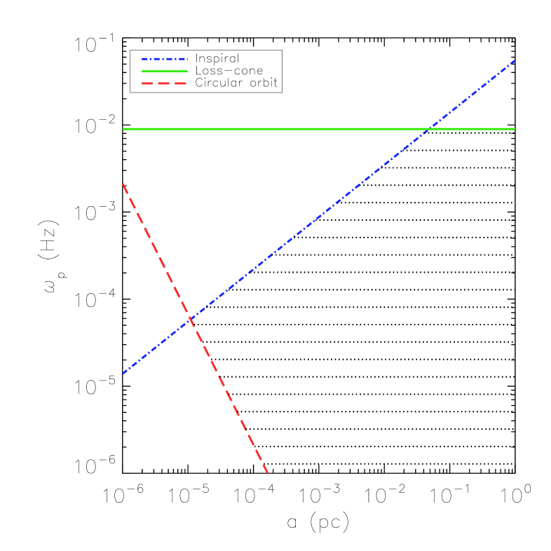
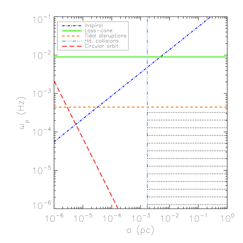
(a)	(b)

Figure 1: Boundaries in orbit space around a MBH of $M_{\bullet}=10^{6}M_{\odot}$ for a BH of $M_{\star}=10M_{\odot}$ in Fig. 1a and of a MS of $M_{\star}=1M_{\odot}$ in Fig. 1b. Stellar orbits are populated in the shaded area only. The figures are representative of all relevant stars and MBHs where the cuts scale according to Eq. (12), (13), (14) and (16). The red line indicates the boundary in orbit space resulting from the condition $r_{p}\leqslant a$. The result is not very sensitive to the inner cutoff; imposing a hard cutoff at $10^{-4}$ pc in figure (a) decreases $(fS_{\rm GW})^{1/2}$ by $\sim 50$ per cent.

3 Gravitational wave background

3.1 Gravitational wave energy in a single burst

For an eccentric Newtonian orbit, the amount of energy emitted in GWs in one period $\Delta E_{\rm GW}$ [see Eq. (7)] and the distribution of this energy over frequencies $dQ/df$ is studied by Peters & Mathews (1963). The emitted power peaks at a frequency $f$ that is twice the circular frequency at periapse $\omega_{p}$. To simplify our analysis we assume that all energy $\Delta E_{\rm GW}$ is emitted at $f=2\omega_{p}$, therefore

$$\dfrac{dQ}{df}=\Delta E_{\rm GW}\ \delta(f-2\omega_{p}).$$ (17)

In reality, the spectrum is quite broad, but the exact shape of the spectrum is not important, since we sum over a very large number of bursts.

3.2 Gravitational wave energy density

We next integrate this spectrum over $M_{\bullet}$ with the space number density of MBHs of Allen & Richstone (2002), which we assume to be constant throughout the history of the Universe,

$$\dfrac{dn_{\bullet}}{dM_{\bullet}}=\dfrac{10^{7}}{M_{\bullet}}\ \mathrm{Gpc}^{-3}\quad\quad\left(10^{5}\ M_{\odot}<M_{\bullet}<10^{8}\ M_{\odot}\right).$$ (18)

The upper boundary comes from a sharp drop in the observed MBH number density around $M_{\bullet}\approx 10^{8}\ M_{\odot}$. Due to a lack of information on MBHs of $M_{\bullet}<10^{6}\ M_{\odot}$, the lower boundary is arbitrarily chosen to be $10^{5}\ M_{\odot}$. Although at frequencies between $10^{-3}$ and $10^{-2}$ Hz, MBHs of the lowest masses contribute most to the EMBB, decreasing the lower bound only mildly affects the EMBB. The energy density of GW bursts emitted by stars of species $M$ is

$$\dot{\mathcal{E}}(f)=\int\limits_{\mathcal{V}}\dfrac{d^{2}\Gamma_{M}}{da\ d\omega_{p}}\ \Delta E_{\rm GW}\ \delta(f-2\omega_{p})\ \dfrac{dn_{\bullet}}{dM_{\bullet}}\ dM_{\bullet}\ d\omega_{p}\ da.$$ (19)

3.3 Observed gravitational wave energy density

The GW spectrum observed by LISA is the accumulation of the GW radiation of all galaxies in the universe. The emitted spectrum $\dot{\mathcal{E}}(f_{\rm em})df_{\rm em}$ is the rate per unit proper time and per unit co-moving volume at which GW energy in the frequency range $(f_{\rm em},f_{\rm em}+df_{\rm em})$ are emitted. The total GW energy density $(d\rho/df)df$ today with frequencies $f=f_{\rm em}/(1+z)$ in the range $(f,f+df)$ is then

$${d\rho\over df}df = df_{\rm em}\int dz\dfrac{dt}{dz}\frac{\dot{\mathcal{E}}(f_{\rm em})}{1+z}$$ (20)

$$= df\int dz\dfrac{dt}{dz}\dot{\mathcal{E}}[f(1+z)].$$

For $0<z<2$, we follow Barack & Cutler (2004) in approximating $t\approx t_{0}\ (1+z)^{-1.18}$, where a spatially flat Friedmann-Lemaître-Robertson-Walker Universe is assumed with $\Omega_{\Lambda}=0.70$ and $\Omega_{M}=0.30$ and the Universe’s current age is $t_{0}=0.964H_{0}^{-1}=1.39\times 10^{10}h_{70}^{-1}$ yr. For sources in the range $0<z<2$, this is accurate to within $\sim$3 per cent. The approximation is justified since the EMBB is dominated by the nearby universe and contributions from $1<z<2$ accounts for just 5-8 per cent of that of $0<z<2$.

3.4 Gravitational wave background for LISA

The energy density of an isotropic background of individually unresolvable GW sources is related to the spectral density in the LISA detector by $S_{\rm GW}(f)=4G/(\pi c^{2}f^{2})\ d\rho_{M}/df$ (Barack & Cutler, 2004), or

$$S_{\rm GW}(f)=\dfrac{4G}{\pi c^{2}f^{2}}\ \int\limits_{\mathcal{V}} dz\ dM_{\bullet}\ d\omega_{p}\ da\ \dfrac{dt}{dz}\dfrac{dn_{\bullet}}{dM_{\bullet}}\dfrac{d^{2}\Gamma_{M}}{da\ d\omega_{p}}\$$ (21)

$$\times\ \Delta E_{\rm GW}\ \delta[f(1+z)-2\omega_{p}]$$

where equations (19) and (20) were used. The integral is taken over $\mathcal{V}$ representing that part of orbit space that is populated according to §2.2.

4 Results

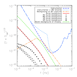
Figure 2: Comparison between the EMBB, instrumental noise of LISA (Larson 2001), the galactic WD binary background (Larson 2001) and the BH EMRI (inspiral) background (Barack & Cutler 2004) with an inspiral rate of $10^{-7}{\rm yr^{-1}}$. The EMBB is smaller than the other types of GW noise. The EMBB due to only BHs, WDs, NSs or MSs is shown in symbols and contributions from BHs dominate the spectrum. The EMBB of the O’Leary et al. (2008) model is also shown. Even though it is significantly higher than the EMBB in our preferred model, it is still lower than the instrumental noise of LISA.

For our main model, the resulting EMBB $(fS_{\rm GW})^{1/2}$ of the four species of stars is shown in figure (2). The EMBB is dominated by contributions from BHs. This is mainly due to two reasons. First, a single burst emitted by a BH is more energetic than a burst emitted by the other species of stars in a similar orbit. Second, the BH distribution is steeper due to mass-segregation which leads to a higher burst rate, see Eq. (2.1). Note that the EMBB due to MSs is cut off at $\sim 10^{-3}$ Hz, because tidal effects prohibit the existence of non-compact objects at small distances from the MBH.

The EMRI background is caused by BHs that spiral in to the MBH. These sources are excluded in our calculations by eliminating inspiral orbits, see §2.2.1. The expression for the EMRI background was taken from Barack & Cutler (2004) and scales with the inspiral rate. From Hopman & Alexander (2006b) we take an inspiral rate of $1\times 10^{-7}$ yr^-1 leading to a EMRI background at a level comparable to the instrumental noise of LISA.

In our favoured model the EMBB is well below the instrumental noise of LISA. At closest approach the EMBB $(fS_{\rm GW})^{1/2}$ is a factor $\sim$ 10 below the instrumental noise of LISA, and a factor $\sim$ 19 lower than the confusion noise of Galactic WD binaries. The EMBB is also lower than the EMRI background in the interesting frequency range where the noise from EMRIs is stronger than that of the instrument itself.

The O’Leary et al. (2008) model is also displayed in figure (2). In this model there are more, and more massive BHs, which raises the EMBB due to an increase in the number of BH bursts and an increase in the relaxation rate protecting stars from inspiral. Figure (2) shows the EMBB is raised by a factor $\sim 6$ on average with respect to our main model. However, even with this stellar distribution the EMBB is smaller than the instrumental noise of LISA by a factor $\sim 1.5$, and a factor $\sim 3$ including the noise of galactic WD binaries. Overall the sensitivity of the EMBB on the individual model parameters is not strong enough to raise the EMBB above the instrumental noise of LISA, without increasing $M_{\mathrm{BH}}$ by a factor 10 and other parameters by even more.

5 Summary and discussion

Stars whose orbits carry them near the Schwarzschild radius of a MBH emit gravitational waves in the LISA frequency band. If the orbit of the star is very eccentric, the star emits bursts of GWs each peri-centre passage without necessarily spiraling in. Most extra-galactic bursts are not individually resolvable and hence will constitute a gravitational wave background.

For our favoured model the EMBB is dominated by GW bursts from BHs, and is a factor $\sim 10$ lower than the instrumental noise of LISA. Including the WD Galactic background increases the insignificance of the EMBB to a factor $\sim 19$. Even for the O’Leary et al. (2008) model, which has a much flatter mass function, the EMBB is smaller than the instrumental noise of LISA by a factor $\sim 1.5$ (or a factor $\sim 3$ including the WD Galactic background). The EMBB is also well below the EMRI background (Barack & Cutler 2004). We conclude that the detection of GWs by LISA will not be hindered by a background of bursting sources.

As an additional application of our model, we revisit the possibility of direct detection of GW bursts in the Galactic centre, due to stars on relativistic orbits. Yunes et al. (2008) have investigated the impact of including relativistic corrections to the description of the star’s trajectory. The degree to which the relativistic corrections are important depends on the star’s orbit and is largest for small peri-centre distances. Yunes et al. (2008) find that orbits with peri-centre velocities $|v_{p}|>0.25c$ account for approximately half of the events within the orbit space considered by Rubbo et al. (2006) around a MBH of $3.7\times 10^{6}\ M_{\odot}$. However, Rubbo et al. (2006) incorporate tight, possibly relativistic orbits that are unpopulated according to our assumptions of the boundaries in orbitspace of §2.2 (see also the appendix). Assuming our main model of a galactic nucleus, a similar MBH mass as Rubbo et al. (2006) and integrating over all frequencies that can be detected by LISA (See Eq. (4) in Hopman et al. (2007) with a signal to noise of 5), relativistic orbits account for $\sim 1$ per cent of all events within the orbit space considered by our main model. We conclude that LISA is unlikely to detect relativistic bursts from the Galactic centre.

Appendix A Depletion of phase space due to gravitational wave inspiral

Throughout this paper, we have not considered the contribution of stars in the region where $t_{J}>t_{i}$ (see §2.2.1). Stars in this region do contribute to the EMBB: these stars spiral in and become eventually directly resolvable EMRIs. Before they can be resolved, however, they contribute to a stochastic background. This contribution to the EMBB was studied by Barack & Cutler (2004), and we find that it is dominant over the contribution of fly-bys (see figure 1).

We stress that our analysis as presented in this paper does not apply to the region $t_{J}>t_{i}$, because orbits in this region are less likely to be populated. In this appendix we analyse a toy model of Monte Carlo (MC) simulations based on the method by Shapiro & Marchant (1978) to show this. For details on the method, we refer to Shapiro & Marchant (1978) and Hopman (2009). The model does not include mass-segregation, and is not intended to faithfully represent a galactic nucleus, but is instead used to highlight the difference in the dynamics in the two regimes delineated by $t_{j}=t_{i}$.

Consider the following simple dynamical model:

Energy diffusion — Let the (scaled) energy $x$ perform a random walk such that the diffusion coefficient is

$$D_{xx}=85x^{9/4}.$$ (22)

The form of this coefficient is such that it reproduces the Bahcall & Wolf (1976) solution with distribution function $f(x)\propto x^{1/4}$; the prefactor is for consistency with Hopman (2009). (Here positive energy implies that the star is bound to the MBH).

Angular momentum diffusion — Let the angular momentum $j$ be scaled by the circular angular momentum, such that by definition $0<j<1$. Let $j$ perform a random walk such that the diffusion coefficient is (see Hopman (2009) for the prefactor)

$$D_{jj}=6.6x^{1/4}.$$ (23)

Boundary conditions — Let the actual angular momentum of the loss-cone be independent of energy, such that if it is scaled by the circular angular momentum, it becomes

$$j_{lc}(x)=\left({x\over x_{\rm max}}\right)^{1/2},$$ (24)

with $x_{\rm max}$ some maximal energy.

Energy loss by GWs — Let the loss of energy per unit time be

$$\dot{x}_{\rm GW}=x^{3/2}\left({j\over j_{lc}(x)}\right)^{-7}\tau^{-1},$$ (25)

which has a scaling such as that in GW emission, and the constant $\tau$ is chosen here to be $\tau=10^{-6}$.

This leads to the following dynamical equations

$$j_{t+\delta t}=j_{t}+r\sqrt{D_{jj}\delta t};$$ (26)

$$x_{t+\delta t}=x_{t}+r\sqrt{D_{xx}\delta t}+\dot{x}_{\rm GW}\delta t,$$ (27)

where in these equations $r$ is a normally distributed random variable with mean zero and unit variance. The three terms in the dynamical equations give rise to three time-scales: the time scale for changes in $j$ of order of itself due to scattering

$$t_{j}=D_{jj}^{-1}j^{2}=(1/6.6)x^{-1/4}j^{2};$$ (28)

the time scale for changes in $x$ of order of itself due to scattering

$$t_{x}=D_{xx}^{-1}x^{2}=(1/85)x^{-1/4};$$ (29)

and the time for changes in $x$ of order of itself due to GW emission

$$t_{i}={x\over\dot{x}_{\rm GW}}=x^{-4}j^{7}x_{\rm max}^{7/2}\tau.$$ (30)

We simulate the dynamical process described above with and without GW emission by means of a MC simulation with about $10^{6}$ particles. We follow the Shapiro & Marchant (1978) cloning scheme in order to resolve the distribution function over several orders of magnitude. We define the distribution $f(x,j^{2})$ as

$$f(x,j^{2})\equiv{x^{5/4}\over j^{2}}{d^{2}N(x,j^{2})\over d\ln xd\ln j^{2}},$$ (31)

where $N$ is the normalised number of particles and the prefactor $x^{5/4}/j^{2}$ was added in order to divide out the dependence on energy and angular momentum if the distribution is isotropic and there are no GWs. We show the resulting normalised steady state distribution in figure (3) for the case without GW emission and figure (4) for the case with GW emission. The figures clearly shows that the region where $t_{i}<t_{j}$ is depleted if there are energy losses to GWs.

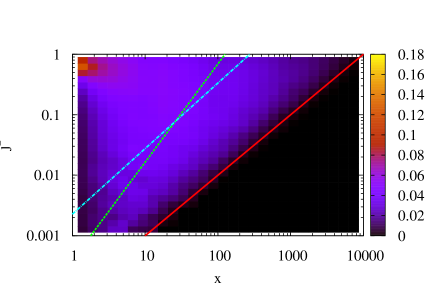
Figure 3: Distribution $f(x,j^{2})$ of stars without GW emission (arbitrary scale). The red solid line denotes the loss-cone, the blue dotted line delineates $t_{j}=t_{i}$, and the green dashed line delineates $t_{x}=t_{i}$.

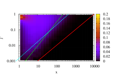
Figure 4: Same as previous figure, but now with energy losses to GWs. Comparison of the two figures shows that the distribution is depleted in presence of GW emission, approximately in the region where $t_{i}<\min(t_{j},t_{x})\sim t_{j}$. Note that some stars do remain within the $t_{i}<\min(t_{j},t_{x})$ region; these are inspiraling stars, and their contribution to the EMBB was accounted for by Barack & Cutler (2004).

References

- Alexander & Hopman (2003) Alexander T., Hopman C., 2003, ApJ, 590, L29
- Alexander & Hopman (2009) Alexander T., Hopman C., 2009, ArXiv e-prints, 697, 1861
- Allen & Richstone (2002) Allen M. C., Richstone D., 2002, AJ, 124, 3035
- Amaro-Seoane et al. (2007) Amaro-Seoane, P., Gair, J. R., Freitag, M., Miller, M. C., Mandel, I., Cutler, C. J., Babak, S., 2007, Clas. Quantum Gravity, 24, 113
- Bahcall & Wolf (1976) Bahcall J. N., Wolf R. A., 1976, ApJ, 209, 214
- Bahcall & Wolf (1977) Bahcall J. N., Wolf R. A., 1977, ApJ, 216, 883
- Barack & Cutler (2004) Barack L., Cutler C., 2004, Phys. Rev. D, 70, 122002 Cohn H., Kulsrud R. M., 1978, ApJ, 226, 1087
- Finn & Thorne (2000) Finn L. S., Thorne K. S., 2000, Phys. Rev. D, 62, 124021 Frank J., Rees M. J., 1976, MNRAS, 176, 633
- Freitag (2001) Freitag M., 2001, Clas. Quantum Gravity, 18, 4033
- Freitag (2003) Freitag M., 2003, ApJ, 583, L21
- Freitag & Benz (2005) Freitag M., Benz W., 2005, MNRAS, pp 245
- Freitag et al. (2006) Freitag M., Amaro-Seoane P., Kalogera V., 2006, ApJ, 649, 91
- Gair et al. (2004) Gair J. R., Barack L., Creighton T., Cutler C., Larson S. L., Phinney E. S., Vallisneri M., 2004, Clas. Quantum Gravity, 21, 1595
- Gair (2008) Gair J. R., 2008, ArXiv e-prints (arXiv: 0811.0188)
- Ghez et al. (2008) Ghez A. M., et al., 2008, IAU symposium, 248, 52
- Glampedakis (2005) Glampedakis K., 2005, Clas. Quantum Gravity, 22, 605
- Hils & Bender (1995) Hils D., Bender P. L., 1995, ApJ, 445, L7
- Hopman & Alexander (2005) Hopman C., Alexander T., 2005, ApJ, 629, 362
- Hopman & Alexander (2006a) Hopman C., Alexander T., 2006a, ApJ, 645, 1152
- Hopman & Alexander (2006b) Hopman C., Alexander T., 2006b, ApJ, 645, L133
- Hopman (2006) Hopman C., 2006, astro-ph/0608460
- Hopman (2009) Hopman C., 2009, ArXiv e-prints, arXiv:0906.0374
- Hopman et al. (2007) Hopman C., Freitag M., Larson S. L., 2007, MNRAS, 378, 129
- Ivanov (2002) Ivanov P. B., 2002, MNRAS, 336, 373
- Keshet et al. (2009) Keshet, U., Hopman, C., Alexander, T. 2009, ArXiv e-prints, arXiv:0901.4343
- Larson (2001) Larson S. L., Online Sensitivity Curve Generator, 2001, based on Larson, S. L., Hellings, R. W. & Hiscock, W. A., 2002, Phys.; located at http://www.srl.caltech.edu/shane/sensitivity/ Rev. D, 66, 062001.
- Lightman & Shapiro (1977) Lightman A. P., Shapiro S. L., 1977, ApJ, 211, 244
- Maness et al. (2007) Maness Hl, et al., 2007, 669, 1024
- Merritt & Ferrarese (2001) Merritt D., Ferrarese L., 2001, MNRAS, 320, L30
- Mouawad et al. (2005) Mouawad N., Eckart A., Pfalzner S., Schödel R., Moultaka J., Spurzem R., 2005, Astron. Nachr., 326, 83
- Nayakshin & Sunyaev (2005) Nayakshin S., Sunyaev R., 2005, MNRAS, 364, L23
- O’Leary et al. (2008) O’Leary R. M., Kocsis B., Loeb A., 2008, ArXiv e-prints, 807
- Peebles (1972) Peebles P. J. E., 1972, ApJ, 178, 371
- Peters & Mathews (1963) Peters P. C., Mathews J., 1963, Phys. Rev., 131, 435
- Quinlan et al. (1995) Quinlan G. D., Hernquist L., Sigurdsson S., 1995, ApJ, 440, 554
- Rauch & Tremaine (1996) Rauch K. P., Tremaine S., 1996, New Astron., 1, 149
- Rauch & Ingalls (1998) Rauch K. P., Ingalls B., 1998, MNRAS, 299, 1231
- Rubbo et al. (2006) Rubbo L. J., Holley-Bockelmann K., Finn L. S., 2006, ApJ, 649, L25
- Shapiro & Marchant (1978) Shapiro, S. L., & Marchant, A. B. 1978, ApJ, 225, 603
- Sigurdsson & Rees (1997) Sigurdsson S., Rees M. J., 1997, MNRAS, 284, 318
- Spitzer & Saslaw (1966) Spitzer L. J., Saslaw W. C., 1966, ApJ, 143, 400
- Spitzer (1987) Spitzer, L. 1987, Dynamical evolution of globular clusters, ed. L. Spitzer
- (43) Tremaine S., et al., 2002, ApJ, 574, 704
- Young (1980) Young P., 1980, ApJ, 242, 1232
- Yunes et al. (2008) Yunes N., Sopuerta C. F., Rubbo L. J., Holley-Bockelmann K., 2008, ApJ, 675, 604