Threshold corrections to the $\gamma t\bar{t}$ vertex at ${\cal O}(\alpha\alpha_{s})$

Abstract

In these proceedings a recent calculation of the last missing piece of the two-loop ${\cal O}(\alpha\alpha_{s})$ corrections to $\gamma t\bar{t}$ vertex at the $t\bar{t}$ threshold due to the exchange of a $W$ boson and a gluon is summarised. The calculation constitutes a building block of the top quark threshold production cross section at electron positron colliders.

1 Introduction

The measurement of the total $t\bar{t}$ cross section constitutes a major part of the top physics program at a future $e^{+}e^{-}$ International Linear Collider (ILC). Due to the large top quark mass and the large width $\Gamma_{t}\gg\Lambda_{QCD}$, non perturbative effects are strongly suppressed at energies around the threshold. Therefore it is possible to determine top quark properties like the mass $m_{t}$ and the width $\Gamma_{t}$, but also the strong coupling $\alpha_{s}$ with high precision. In Ref. [2] it has been shown that an uncertainty of below 100 MeV can be obtained for $m_{t}$ from a threshold scan of the cross section.

The feasibility of such high-precision measurements requires a theory prediction of the total cross section $\sigma(e^{+}e^{-}\rightarrow t\bar{t})$ with high accuracy (preferably $\delta\sigma/\sigma\leq 3\%$). The study of $t\bar{t}$ threshold production is performed in the framework of non-relativistic QCD (NRQCD) [3] which separates the hard and soft scales involved in the process. The next-to-next-to-leading order (NNLO) calculation [4] turned out to be as large as the NLO one. Only the (partial) NNNLO [5, 6] results show a good convergence of the perturbative expansion and a strong reduction of the scale dependence from NNLO to NNNLO can be observed. The remaining uncertainty turns out to be of the order of 10%. A similar value is obtained from the approach based on the resummation of logarithmically enhanced terms which have been considered in Refs. [7, 8].

In order to reach a theory goal of $\delta\sigma/\sigma\leq 3\%$ it is necessary to include in the prediction next to the one-loop electroweak corrections, which are known since quite some time [9] (see also [10]), also higher order effects. The evaluation of ${\cal O}(\alpha\alpha_{s})$ corrections has been started in Ref. [11], where the two-loop mixed electroweak and QCD corrections to the matching coefficient of the vector current has been computed due to a Higgs or $Z$ boson exchange in addition to a gluon. In these proceedings the calculation of ${\cal O}(\alpha\alpha_{s})$ for the two-loop vertex diagrams mediated by a $W$ boson and gluon exchange is summarised [12]. This result completes the vertex corrections of order $\alpha\alpha_{s}$ — a building block for the top quark production cross section. Assuming the (numerically well justified) power counting $\alpha\sim\alpha_{s}^{2}$ one can see that these corrections are formally of NNNLO.

In order to complete the matching corrections of order $\alpha\alpha_{s}$ also the two-loop box diagrams contributing to $e^{+}e^{-}\to t\bar{t}$ have to be considered. Actually, only the proper combination of the box, vertex and self-energy contributions (the latter can, e.g., be found in Refs. [13, 14]) forms a gauge independent set.

2 Threshold cross section

Within the framework of NRQCD [3] the total cross section for the top quark production can be cast in the form

$$R\left(e_{L}^{+}e_{R}^{-}\rightarrow t\bar{t}X\right) = \frac{8\pi}{s}\,{\rm Im}\big{[}\,\left(h_{R,V}\right)^{\,2}H_{V}+\left(h_{R,A}\right)^{\,2}H_{A}\big{]}\,,$$ (1)

where $s$ is the square of the centre-of-mass energy and $R(e_{L}^{+}e_{R}^{-}\rightarrow t\bar{t}X)$ is the cross section normalised to $\sigma(e^{+}e^{-}\rightarrow\mu^{+}\mu^{-})=(4\pi\alpha^{2})/(3s)$. For illustration we consider in Eq. (1) left-landed positrons and right-handed electrons. For $e^{+}_{R}e^{-}_{L}$ in the initial state a similar expression is obtained by replacing R by L in Eq. (1). Note that in the SM the initial states $e^{+}_{R}e^{-}_{R}$ and $e^{+}_{L}e^{-}_{L}$ are suppressed by a factor $(m_{e}/M_{W})^{2}\sim 10^{-10}$ and are thus negligible. We denote $h_{R,V}$ and $h_{R,A}$ by helicity amplitudes which absorb the matching coefficients representing the effective coupling of the effective operators. They take care of the hard part of the reaction. The first subscript of $h$ refers to helicity of the electron, and the second one to the vector ($J_{V}^{\mu}=\bar{\psi}\gamma^{\mu}\psi$) or axial-vector coupling ($J_{A}^{\mu}=\bar{\psi}\gamma^{\mu}\gamma_{5}\psi$) of the gauge bosons to the top quark current. The bound-state dynamics is contained in the so-called hadronic part which is denoted by $H_{V}$ and $H_{A}$ in Eq. (1).

In the cross section formula (1) “${\rm Im}$” refers to those cuts which correspond to the $t\bar{t}X$ final state. This means that we have to select special cuts which correspond to the final state we are interested in. This requires a dedicated study incorporating the experimental setup. For the one-loop electroweak correction this treatment was performed in [15]. In [12] we did not pursue this problem further.

The evaluation of $H_{V}$ and $H_{A}$ requires to integrate out the low-energy modes of QCD, the soft, potential and ultrasoft gluons contained in NRQCD [16, 17]. For the top quark system this can be done perturbatively. In a first step one integrates out the soft and potential gluons which results in the effective field theory Potential NRQCD [18, 19]. The

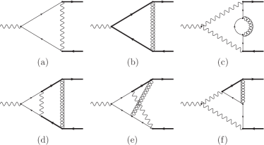
Figure 1: Sample Feynman diagrams contributing to the matching coefficient of the vector current at order $\alpha$ (a), $\alpha_{s}$ (b) and $\alpha\alpha_{s}$ (c)-(f). The thick (thin) straight lines represent top (bottom) quarks, wavy lines stand for $W$ bosons and the curly ones for gluons.

corresponding Lagrangian is known to NNNLO [20]. To integrate out nonrelativistic top and anti-top quark fields the Rayleigh-Schrödinger perturbation theory can be applied as was initiated in Ref. [22] and performed to NNNLO for $H_{V}$ and $H_{A}$ in Refs. [6] and [23], respectively. Integrating out the ultrasoft gluon was completed recently in Ref. [5]. For the details of these steps we refer to the original papers and references cited therein (see also Refs. [24, 25, 26, 27, 28]).

In these proceedings we report on a recent publication, where corrections of ${\cal O}(\alpha\alpha_{s})$ to $h_{I,F}$ were computed. Some sample vertex diagrams which have to be evaluated at threshold are shown in Fig. 1. Let us mention that the corresponding two-loop QCD corrections have been presented in Refs. [29, 30] and the three-loop corrections induced by a light quark loop in Ref. [31].

3 Calculation of the vertex diagrams

The two-loop diagrams which have to be evaluated are generated with QGRAF [32] and further processed with q2e and exp [33, 34]. The reduction of the integrals is performed with the program crusher [35] which implements the Laporta algorithm [36, 37]. We arrive at 29 master integrals (MI). Some MIs factorise into one-loop integrals or contain only one dimensionful scale. Most of these integrals are available in the literature and can, e.g., be found in Refs. [38, 39, 40, 41, 11, 42].

The two-scale MIs are evaluated via an expansion in $z=M_{W}^{2}/m_{t}^{2}$. A promising method to obtain the results is based on differential equations (see Ref. [43] for a recent review) which provide the expansion in an automatic way once the initial conditions are specified. With the help of the ansatz

$$\text{MI}=\sum c_{ijk}\,\epsilon^{i}z^{j}(\ln z)^{k},$$ (2)

the differential equations can be expanded in $\epsilon$ and $z$. As a result they reduce to algebraic equations for the coefficients $c_{ijk}$, which can be solved trivially. In every order in $\epsilon$ there is one constant $c_{ijk}$ which can not be determined with this procedure. It is obtained from the initial condition at $z=0$. Unfortunately, we could not get analytic results for five coefficients in the $\epsilon$-expansion of four MIs at $z=0$. We calculated these coefficients using the Mellin-Barnes method (see, e.g., Ref [44]) where we used the program packages AMBRE [45] and MB [46].

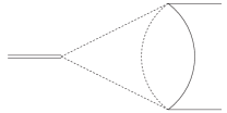
Figure 2: Solid(dotted) lines correspond to propagators with mass $m_{t}$(0). Single external lines are on the mass shell with mass $m_{t}$ whereas double external line have mass $2m_{t}$.

The Mellin-Barnes representation for a given integral is not unique. In particular it might happen that the convergence of the resulting numerical integration turns out to be good in one case whereas a poor convergence is observed in other cases. The crucial quantity in this respect is the asymptotic behaviour of the $\Gamma$ function for large imaginary part which is given by

$$\Gamma(a\pm ib)\stackrel{{\scriptstyle\tiny b\to\infty}}{{\simeq}}\sqrt{2\pi}e^{\pm i\frac{\pi}{4}(2a-1)}e^{\pm ib(\ln b-1)}e^{-\frac{b\pi}{2}}b^{a-\frac{1}{2}}\,,$$ (3)

where the first two exponential factors lead to oscillations. Let us discuss this in more detail for the Mellin-Barnes representation of one of the MIs, which is depicted in Fig. 2:

MI $$= \left(\frac{e^{\gamma_{E}}\mu^{2}}{m_{t}^{2}}\right)^{2\epsilon}\int_{-i\infty}^{+i\infty}\frac{dz_{1}}{2\pi i}\int_{-i\infty}^{+i\infty}\frac{dz_{2}}{2\pi i}\,e^{i\pi(2\epsilon+z_{1})}4^{-2\epsilon-z_{2}}$$ (4)

$$\times\frac{\Gamma(1-\epsilon)\Gamma(-\epsilon-z_{1}+1)\Gamma(-z_{1})\left[\Gamma(-2\epsilon-z_{2}+1)\right]^{2}}{\Gamma(-3\epsilon-z_{1}+2)\Gamma(-2\epsilon-z_{1}+2)\Gamma(-4\epsilon-2z_{2}+2)}$$

$$\times\Gamma(-4\epsilon-z_{1}-z_{2}+2)\Gamma(z_{1}-z_{2})\Gamma(\epsilon+z_{2})\Gamma(2\epsilon+z_{2})\,,$$

where $\gamma_{E}=0.577216\dots$ and the contour of integration is chosen in such a way that the poles of the $\Gamma$ functions with $+z_{i}$ are separated from the poles of the $\Gamma$ functions with $-z_{i}$. Using the package MB we can expand the integrand in $\epsilon$. For the finite contribution this leads to a sum of an analytic part, a one-dimensional Mellin-Barnes integral and a two-dimensional one. The latter correspond to the integral in Eq. (4) for $\epsilon=0$. If we insert in this expression the asymptotic behaviour for the $\Gamma$ functions as given in Eq. (3) one observes that the integrand of the two-dimensional integral falls off exponentially, except for $\mbox{Im}(z_{2})=0,\mbox{Im}(z_{1})<0$. On this line the drop-off only shows a power-law behaviour which is dictated by the last factor of Eq. (3). In our particular case the drop-off turns out to be extremely slow for the integration contour chosen by MB which corresponds to $\mbox{Re}(z_{1})=-1/4$ and $\mbox{Re}(z_{2})=-1/2$. Thus it is hard to get an accurate result by the numerical integration since a highly oscillating functions has to be integrated. A closer look to the fall-off behaviour in Eq. (3) shows that it is possible to improve the drop-off for Im$(z_{1})\to-\infty$ by taking residues of the integrand in $z_{2}$ and thus shifting the integration contour for $z_{2}$ more and more to positive values for Re$(z_{2})$. In this way the integrand becomes well-behaved and can be integrated numerically with sufficiently high precision.

It has already been pointed out in [46] that for certain kinematical configurations the Mellin-Barnes integrals exhibit poor convergence behaviour. We have shown that at least for the threshold integrals needed in our calculation, it is possible to choose the integration paths in a way to make the numerical integration possible. One may hope that with the approach described here it will turn out to be possible to use Mellin-Barnes integration for other troublesome integrals, too.

The other integrals which were solved using the Mellin-Barnes method show similar properties than the MI above. In all cases it is possible to end up with integrals which could be integrated numerically. The accuracy for the finite part of these integrals is sufficient to obtain the final result with four significant digits.

Note that contrary to the default settings of MB we do not use Vegas for the multidimensional numerical integrations. Instead we use Divonne which is available from the Cuba library [47]. For the integrals we have considered it leads to more accurate results using less CPU time.

We have performed an independent check of the initial conditions for all the MIs employing the method of sector decomposition. In particular we used the program FIESTA [48].

4 Results

The hard part of the cross section in (1) at tree level is given by

$$h_{I,V/A}^{\rm tree} = Q_{e}Q_{t}+\frac{s\,\beta_{I}^{\,e}\,\beta_{V/A}^{\,t}}{s-M_{Z}^{2}}~{}~{}~{}{\rm with}~{}~{}\beta_{V/A}^{\,t}=\frac{\beta_{R}^{\,t}\pm\beta_{L}^{\,t}}{2},$$ (5)

where the $\beta_{I}^{\,f}$ is the coupling of a fermion ($f=e,t$) with helicity $I$ to the $Z$ boson [12]. We denote by $\Gamma_{A}^{\,t}$ the contribution of the sum of all one-particle-irreducible diagrams to the $\gamma t\bar{t}$ vertex and parametrise the radiative corrections in the form

$$\hat{\Gamma}_{A}^{\,t}=Q_{t}+{\hat{\Gamma}}_{A}^{\,t,\,(0,1)}+{\hat{\Gamma}}_{A}^{\,t,\,(1,0)}+\hat{\Gamma}_{A}^{\,t,\,(1,1)}\,,$$ (6)

where the hat denotes renormalised quantities and the subscripts $(i,j)$ indicate corrections of ${\cal O}(\alpha^{i}\alpha_{s}^{j})$. Substituting $\hat{\Gamma}_{A}^{\,t}$ for the $Q_{t}$ in Eq. (5) and retaining the relevant orders in the electroweak and strong couplings leads to the corrections to the helicity amplitudes, $h_{I,V}^{(0,1)},h_{I,V}^{(1,0)}$ and $h_{I,V}^{(1,1)}$. We further decompose $\hat{\Gamma}_{A}^{\,t}$ (and similarly the quantities on the right-hand side of Eq. (6)) according to the contributions from the Higgs, $Z$ and $W$ boson exchanges:

$$\hat{\Gamma}_{A}^{\,t}=\hat{\Gamma}_{A,H}^{\,t}+\hat{\Gamma}_{A,Z}^{\,t}+\hat{\Gamma}_{A,W}^{\,t}\,.$$ (7)

The results for the electroweak corrections read [9, 11, 12]

$$\hat{\Gamma}_{A,H}^{t,(1,0)}=21.1\times 10^{-3}~{}(10.6\times 10^{-3})~{}~{}~{}\mbox{for}~{}~{}M_{H}=120~{}(200)~{}{\rm GeV}\,,$$

$$\hat{\Gamma}_{A,W}^{t,(1,0)}=3.0\times 10^{-3}\,,$$

$$\hat{\Gamma}_{A,Z}^{t,(1,0)}=1.7\times 10^{-3}\,,$$

$$\hat{\Gamma}_{A,H}^{t,(1,1)}=-17.6\times 10^{-3}~{}(-6.6\times 10^{-3})~{}~{}~{}\mbox{for}~{}~{}M_{H}=120~{}(200)~{}{\rm GeV}\,,$$

$$\hat{\Gamma}_{A,W}^{t,(1,1)}=0.2\times 10^{-3}\,,$$

$$\hat{\Gamma}_{A,Z}^{t,(1,1)}=-1.0\times 10^{-3}\,.$$ (8)

One observes quite small corrections from the $W$ and $Z$ boson induced contributions. From Eq. (8) one can read off that relatively big one-loop effects are obtained for light Higgs boson masses. However, there is a strong cancellation between the one- and two-loop terms resulting in corrections which have the same size as the sum of the one- and two-loop contributions of the $W$ and $Z$ boson diagrams. In general moderate effects are observed suggesting that in the electroweak sector perturbation theory works well, which is in contrast to the pure QCD corrections. Let us in the end mention that $\hat{\Gamma}_{A,W}^{t,(1,1)}$ leads to a correction of $0.1\%$ to $R$.

5 Acknowledgements

Y. Kiyo and M. Steinhauser are gratefully acknowledged for the collaboration. Diagrams have been drawn with Axodraw/Jaxodraw [49, 50].

References

-
[1]
Presentation:
http://ilcagenda.linearcollider.org/contributionDisplay.py?contribId=91&sessionId=18&confId=2628 - [2] M. Martinez and R. Miquel, Eur. Phys. J. C 27 (2003) 49 [arXiv:hep-ph/0207315].
- [3] G. T. Bodwin, E. Braaten and G. P. Lepage, Phys. Rev. D 51 (1995) 1125 [Erratum-ibid. D 55 (1997) 5853] [arXiv:hep-ph/9407339].
- [4] A. H. Hoang et al., Eur. Phys. J. direct C 2 (2000) 1 [arXiv:hep-ph/0001286].
- [5] M. Beneke, Y. Kiyo and A. A. Penin, Phys. Lett. B 653 (2007) 53 [arXiv:0706.2733 [hep-ph]]; M. Beneke and Y. Kiyo, Phys. Lett. B 668 (2008) 143 [arXiv:0804.4004 [hep-ph]].
- [6] M. Beneke, Y. Kiyo and K. Schuller, PoS RADCOR2007 (2007) 051 [arXiv:0801.3464 [hep-ph]].
- [7] A. H. Hoang, Acta Phys. Polon. B 34 (2003) 4491 [arXiv:hep-ph/0310301].
- [8] A. Pineda and A. Signer, Nucl. Phys. B 762 (2007) 67 [arXiv:hep-ph/0607239].
- [9] R. J. Guth and J. H. Kühn, Nucl. Phys. B 368 (1992) 38.
- [10] A. H. Hoang and C. J. Reisser, Phys. Rev. D 74 (2006) 034002 [arXiv:hep-ph/0604104].
- [11] D. Eiras and M. Steinhauser, Nucl. Phys. B 757 (2006) 197 [arXiv:hep-ph/0605227].
- [12] Y. Kiyo, D. Seidel and M. Steinhauser, JHEP 0901 (2009) 038 [arXiv:0810.1597 [hep-ph]].
- [13] B. A. Kniehl, Nucl. Phys. B 347 (1990) 86.
- [14] A. Djouadi and P. Gambino, Phys. Rev. D 49 (1994) 3499 [Erratum-ibid. D 53 (1996) 4111] [arXiv:hep-ph/9309298].
- [15] A. H. Hoang and C. J. Reisser, Phys. Rev. D 71 (2005) 074022 [arXiv:hep-ph/0412258].
- [16] M. E. Luke and M. J. Savage, Phys. Rev. D 57 (1998) 413 [arXiv:hep-ph/9707313].
- [17] M. Beneke and V. A. Smirnov, Nucl. Phys. B 522 (1998) 321 [arXiv:hep-ph/9711391].
- [18] A. Pineda and J. Soto, Nucl. Phys. Proc. Suppl. 64 (1998) 428 [arXiv:hep-ph/9707481].
- [19] N. Brambilla, A. Pineda, J. Soto and A. Vairo, Nucl. Phys. B 566 (2000) 275 [arXiv:hep-ph/9907240].
- [20] B. A. Kniehl, A. A. Penin, V. A. Smirnov and M. Steinhauser, Nucl. Phys. B 635 (2002) 357 [arXiv:hep-ph/0203166].
- [21] A. V. Smirnov, V. A. Smirnov and M. Steinhauser, Phys. Lett. B 668 (2008) 293 [arXiv:0809.1927 [hep-ph]].
- [22] V. S. Fadin and V. A. Khoze, JETP Lett. 46 (1987) 525 [Pisma Zh. Eksp. Teor. Fiz. 46 (1987) 417].
- [23] A. A. Penin and A. A. Pivovarov, Phys. Atom. Nucl. 64 (2001) 275 [Yad. Fiz. 64 (2001) 323] [arXiv:hep-ph/9904278].
- [24] B. A. Kniehl and A. A. Penin, Nucl. Phys. B 563 (1999) 200 [arXiv:hep-ph/9907489].
- [25] A. V. Manohar and I. W. Stewart, Phys. Rev. D 63 (2001) 054004 [arXiv:hep-ph/0003107].
- [26] B. A. Kniehl, A. A. Penin, M. Steinhauser and V. A. Smirnov, Phys. Rev. Lett. 90 (2003) 212001 [arXiv:hep-ph/0210161]; Phys. Rev. Lett. 91 (2003) 139903, Erratum.
- [27] A. H. Hoang, Phys. Rev. D 69 (2004) 034009 [arXiv:hep-ph/0307376].
- [28] A. A. Penin, V. A. Smirnov and M. Steinhauser, Nucl. Phys. B 716 (2005) 303 [arXiv:hep-ph/0501042].
- [29] A. Czarnecki and K. Melnikov, Phys. Rev. Lett. 80 (1998) 2531 [arXiv:hep-ph/9712222].
- [30] M. Beneke, A. Signer and V. A. Smirnov, Phys. Rev. Lett. 80 (1998) 2535 [arXiv:hep-ph/9712302].
- [31] P. Marquard, J. H. Piclum, D. Seidel and M. Steinhauser, Nucl. Phys. B 758 (2006) 144 [arXiv:hep-ph/0607168].
- [32] P. Nogueira, J. Comput. Phys. 105 (1993) 279.
- [33] R. Harlander, T. Seidensticker and M. Steinhauser, Phys. Lett. B 426 (1998) 125 [hep-ph/9712228].
- [34] T. Seidensticker, hep-ph/9905298.
- [35] P. Marquard and D. Seidel, unpublished.
- [36] S. Laporta and E. Remiddi, Phys. Lett. B 379 (1996) 283 [arXiv:hep-ph/9602417].
- [37] S. Laporta, Int. J. Mod. Phys. A 15 (2000) 5087 [arXiv:hep-ph/0102033].
- [38] R. Scharf and J. B. Tausk, Nucl. Phys. B 412 (1994) 523.
- [39] J. Fleischer, F. Jegerlehner, O. V. Tarasov and O. L. Veretin, Nucl. Phys. B 539 (1999) 671 [Erratum-ibid. B 571 (2000) 511] [arXiv:hep-ph/9803493].
- [40] D. Seidel, Phys. Rev. D 70 (2004) 094038 [arXiv:hep-ph/0403185].
- [41] M. Y. Kalmykov, JHEP 0604 (2006) 056 [arXiv:hep-th/0602028].
- [42] J. H. Piclum, “Heavy quark threshold dynamics in higher order,” Dissertation, Hamburg University, 2007.
- [43] M. Argeri and P. Mastrolia, Int. J. Mod. Phys. A 22 (2007) 4375 [arXiv:0707.4037 [hep-ph]].
- [44] V. A. Smirnov, “Evaluating Feynman Integrals,” Springer Tracts Mod. Phys. 211 (2004) 1.
- [45] J. Gluza, K. Kajda and T. Riemann, Comput. Phys. Commun. 177 (2007) 879 [arXiv:0704.2423 [hep-ph]].
- [46] M. Czakon, Comput. Phys. Commun. 175 (2006) 559 [arXiv:hep-ph/0511200].
- [47] T. Hahn, Comput. Phys. Commun. 168 (2005) 78 [arXiv:hep-ph/0404043].
- [48] A. V. Smirnov and M. N. Tentyukov, arXiv:0807.4129 [hep-ph].
- [49] J. A. M. Vermaseren, Comput. Phys. Commun. 83 (1994) 45.
- [50] D. Binosi, J. Collins, C. Kaufhold and L. Theussl, arXiv:0811.4113 [hep-ph]. D. Binosi and L. Theussl, Comput. Phys. Commun. 161 (2004) 76 [arXiv:hep-ph/0309015].