A general two-cycle network model of molecular motors

Abstract

Molecular motors are single macromolecules that generate forces at the piconewton range and nanometer scale. They convert chemical energy into mechanical work by moving along filamentous structures. In this paper, we study the velocity of two-head molecular motors in the framework of a mechanochemical network theory. The network model, a generalization of the recently work of Liepelt and Lipowsky (PRL 98, 258102 (2007)), is based on the discrete mechanochemical states of a molecular motor with multiple cycles. By generalizing the mathematical method developed by Fisher and Kolomeisky for single cycle motor (PNAS(2001) 98(14) P7748-7753), we are able to obtain an explicit formula for the velocity of a molecular motor.

PACS: 87.16.Nn, 87.16.A-, 82.39.-k, 05.40.Jc

Keywords: molecular motors, mechanochemical network

1 Introduction

In biological cells, molecular motors are individual protein molecules that are responsible for many of the biophysical functions of the cellular movement and mechanics. Important examples of motor proteins are kinesin [1, 2, 3], dynein [4, 5], mysion [6, 7, 8] and $F_{0}F_{1}$-ATP synthase [9]. Molecular motors are mechanochemical force generators which convert biochemical energy (stored as ATP, adenosine triphosphate) into mechanical work in a thermal environment [10, 11]. Many molecular motors, due to their two-head nature and hand-over-hand mechanism, can move processively along their tracks for a long time before its dissociation from the track. For example, myosin slides along an actin filament, kinesin and dynein along microtubule (MT). The velocity of molecular motors is quite fast, with mean velocity at about several hundreds nanometers per second [12]. Understanding how the various molecular motors operate is a significant scientific challenge with important nano-engineering implications.

To understand the principle of molecular motors, a good mathematical model is essential. Much progress has been made in recent years in theoretical analysis of molecular motors. Mainly two different approaches have been taken: The ratchet models that consider motor chemical transitions occur without explicit coupling to motor steppings [13, 14], and the discrete chemical models that contain only a single chemomechanical cycle [15, 16]. Recently, however, Liepelt and Lipowsky [17, 18] introduced a six-state network to model the chemomechanical motor cycles, in which the dynamics of two-head motor molecule is described by a Markovian jump process. In [19], Schmiedl and Seifert used a two states network to discuss the efficiency of the molecular motors. The importance of the latter development is in introducing futile cycles into the discrete chemical model, thus making the discrete chemical approach and continuous Brownian approach more connected. Their results indicate that the network modeling approach is a good choice for the theoretical analysis of the molecular motors. In the past, a great deal of mathematical analysis is based on the Brownian ratchet formalism. Similar network models has also be used successfully in the theoretical analysis of other biochemical processes [20, 21].

In this paper, we shall generalize the network model to include arbitrary $2N$ number of states. In particular, we shall use the network model to analyze the movement of molecular motors. Mathematically, therefore, the models developed in [18, 19] and even those in [20, 21] can be regarded as special cases of our network model. In the framework of this network model, we further develop a method pioneered by Derrida, Fisher and Kolomeisky [22, 23, 24] to compute the mean velocity of a molecular motor.

In our model, a two-head molecular motor with hand-over-hand mechanism is assumed to have $2N$ mechanochemical states in their movement, denoted by $0,1,2,\cdots,2N-1$ (see Figure 1). The two heads moves exactly with half of cycle out of phase. If there are 2N states in the hydrolysis kinetic cycle of a single head; we have states $(0,N),(1,N+1),(2,N+2),\cdots,(2N-2,N-2)$, and $(2N-1,N-1)$ for the motor with two heads. The hand-over-hand mechanism means the motor “walks” a step with the transition $(N,0)\rightarrow(0,N)$, switching the leading and the trailing head. However, it is possible that the translocation does not occur, and the kinetic cycle is completed as a futile cycle, with two ATP hydrolyzed, one by each head.

From now one, we shall use the state of the leading head to denote the state of the motor; and denote the forward and backward rate parameters at state $i$ as $u_{i}$ (i.e., $i\to i+1$) and $w_{i}$ ($i\to i-1$) respectively, which satisfy $u_{2N+i}=u_{i}$ and $w_{2N+i}=w_{i}$ (since molecular motors move forward periodically). Generally, the transition rates $u_{i}$ and $w_{i}$ depend on the external force $F_{ext}$ and the free energy $\triangle G$ released by the fuel molecular. The transition rates between state $N$ and $0$, the hand-over-hand, are $u$ and $w$. In the following, we suppose that all these transition rates are known explicitly.

The transition from $N\to 0$ represents the switching between the leading and trailing heads, thus moves one motor step. If a mechanochemical process takes $0\to 1\to\cdots\to N\to N+1\to\cdots\to 2N-1\to 0$, the molecular motors make no mechanical step while hydrolyzing two ATP. However, if the process takes $0\to 1\to\cdots\to N\to 0\to 1\to\cdots N\to 0$, then the motor hydrolyzed two ATP and moved two steps. It can be readily found that, for $N=3$, this model reduces to the 6 states network model in [17], for $N=1$, this model reduces to the 2 states model in [19].

In the next section, we shall give the formulation of the velocity of molecular motors using the network model. We will discuss some special cases in section 3. The force dependence of the transition rates $u_{i},w_{i}$ and $u,w$ is discussed in section 4. In section 5, we will discuss the continuous mechanochemical sate case of our multi-cycle model, and section 6 contains concluding remarks.

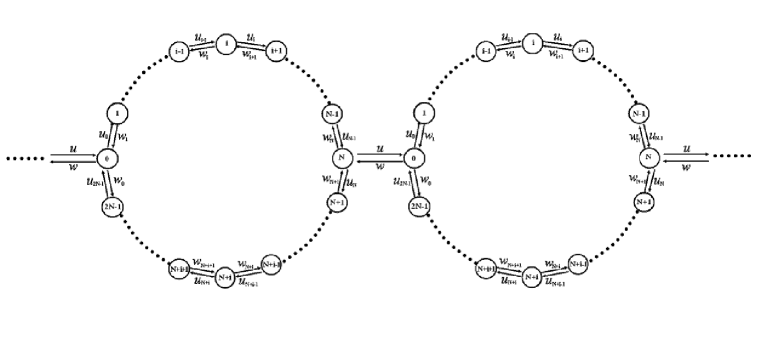
Figure 1: A schematic depiction of the $2N$ states network model for molecular motors. One forward step of molecular motors is completed only in the biochemical process $N\to 0$. In mechanochemical process $0\to 1\to\cdots\to N\to N+1\to\cdots\to 2N-1\to 0$, the molecular motors make no mechanical step while hydrolyzing two ATP.

2 The velocity of molecular motors

In this section, we will calculate the velocity of the molecular motors in the framework of our network model. The method used in the following is similar to the one used in [22, 23] and [24].

Let $\rho_{i}(t)$ be the probability density for finding molecular motors in state $i$ at time $t$. The evolution of the probability density $\rho_{i}(t)$ is governed by the following master equations

$$\frac{d\rho_{i}}{dt}= (\rho_{i-1}u_{i-1}+\rho_{i+1}w_{i+1})-\rho_{i}(u_{i}+w_{i})$$ (1)

$$= (\rho_{i-1}u_{i-1}-\rho_{i}w_{i})-(\rho_{i}u_{i}-\rho_{i+1}w_{i+1})$$

$$\triangleq J_{i}-J_{i+1}\qquad\textrm{for}\ 1\leq i\leq N-1\ \textrm{or}\ N+1\leq i\leq 2N-1$$

and

$$\begin{aligned} \frac{d\rho_{0}}{dt}=&(\rho_{2N-1}u_{2N-1}-\rho_{0}w_{0})-(\rho_{0}u_{0}-\rho_{1}w_{1})+(\rho_{N}u-\rho_{0}w)\cr\triangleq&J_{2N}-J_{1}+J\end{aligned}$$ (2)

$$\begin{aligned} \frac{d\rho_{N}}{dt}=&(\rho_{N-1}u_{N-1}-\rho_{N}w_{N})-(\rho_{N}u_{N}-\rho_{N+1}w_{N+1})-(\rho_{N}u-\rho_{0}w)\cr\triangleq&J_{N}-J_{N+1}-J\end{aligned}$$

where

$$J_{i}=\rho_{i-1}u_{i-1}-\rho_{i}w_{i}\qquad J=\rho_{N}u-\rho_{0}w$$ (3)

$J_{i}$ is the probability flux from mechanochemical state $i-1$ to state $i$, and $J$ is the probability flux from mechanochemical state $N$ to state $0$. At steady state,

$$J_{1}=J_{2}=\cdots=J_{N}\quad J_{N+1}=J_{N+2}=\cdots=J_{2N}\quad J_{1}=J_{2N}+J$$ (4)

By Eqs. (1-4), one can know that

$$\rho_{k}=\rho_{0}\prod_{i=1}^{k}\left(\frac{u_{i-1}}{w_{i}}\right)-\left[1+\sum_{i=1}^{k-1}\prod_{j=i}^{k-1}\left(\frac{u_{j}}{w_{j}}\right)\right]\frac{J_{1}}{w_{k}}$$ (5)

$$\rho_{N+k}=\rho_{N}\prod_{i=1}^{k}\left(\frac{u_{N+i-1}}{w_{N+i}}\right)-\left[1+\sum_{i=1}^{k-1}\prod_{j=i}^{k-1}\left(\frac{u_{N+j}}{w_{N+j}}\right)\right]\frac{J_{1}-J}{w_{N+k}}$$

where $1\leq k\leq N-1$ and

$$\rho_{N}=\rho_{0}\prod_{i=1}^{N}\left(\frac{u_{i-1}}{w_{i}}\right)-\left[1+\sum_{i=1}^{N-1}\prod_{j=i}^{N-1}\left(\frac{u_{j}}{w_{j}}\right)\right]\frac{J_{1}}{w_{N}}$$ (6)

$J_{2N}=J_{1}-J$ means $\rho_{2N-1}u_{2N-1}-\rho_{0}w_{0}=J_{1}-J$, so

$$\rho_{0}= \frac{\rho_{2N-1}u_{2N-1}}{w_{0}}-\frac{J_{1}-J}{w_{0}}$$ (7)

$$= \rho_{N}\prod_{i=1}^{N}\left(\frac{u_{N+i-1}}{w_{N+i}}\right)-\left[1+\sum_{i=1}^{N-1}\prod_{j=i}^{N-1}\left(\frac{u_{N+j}}{w_{N+j}}\right)\right]\frac{J_{1}-(\rho_{N}u-\rho_{0}w)}{w_{0}}$$

Substituting (6) into (7), one obtains

$$\rho_{0}=\frac{A}{B}J_{1}$$ (8)

where

$$A=\left[1+\sum_{i=1}^{2N-1}\prod_{j=i}^{2N-1}\left(\frac{u_{j}}{w_{j}}\right)\right]\frac{1}{w_{0}}+\left[1+\sum_{i=1}^{N-1}\prod_{j=i}^{N-1}\left(\frac{u_{j}}{w_{j}}\right)\right]\left[1+\sum_{i=N+1}^{2N-1}\prod_{j=i}^{2N-1}\left(\frac{u_{j}}{w_{j}}\right)\right]\frac{u}{w_{0}w_{N}}$$ (9)

and

$$B=\left[\frac{u}{w_{N}}\prod_{i=0}^{N-1}\left(\frac{u_{i}}{w_{i}}\right)-\frac{w}{w_{0}}\right]\left[1+\sum_{i=N+1}^{2N-1}\prod_{j=i}^{2N-1}\left(\frac{u_{j}}{w_{j}}\right)\right]+\prod_{i=0}^{2N-1}\left(\frac{u_{i}}{w_{i}}\right)-1$$ (10)

So

$$J=\left\{\left[u\prod_{i=1}^{N}\left(\frac{u_{i-1}}{w_{i}}\right)-w\right]\frac{A}{B}-\left[1+\sum_{i=1}^{N-1}\prod_{j=i}^{N-1}\left(\frac{u_{j}}{w_{j}}\right)\right]\frac{u}{w_{N}}\right\}J_{1}=:CJ_{1}$$ (11)

By (5) (6) (8) (11), we get the expressions of probabities $\rho_{k}$ and $\rho_{N+k}$ as functions of $J_{1}$:

$$\rho_{k}=\left\{\frac{Aw_{0}}{B}\prod_{i=0}^{k-1}\left(\frac{u_{i}}{w_{i}}\right)-\sum_{i=1}^{k-1}\prod_{j=i}^{k-1}\left(\frac{u_{j}}{w_{j}}\right)-1\right\}\frac{J_{1}}{w_{k}}$$ (12)

$$\rho_{N+k}= \left\{\frac{Aw_{0}}{B}\prod_{i=0}^{N+k-1}\left(\frac{u_{i}}{w_{i}}\right)-\sum_{i=1}^{N+k-1}\prod_{j=i}^{N+k-1}\left(\frac{u_{j}}{w_{j}}\right)\right.$$ (13)

$$+\left.C\sum_{i=N+1}^{N+k-1}\prod_{j=i}^{N+k-1}\left(\frac{u_{j}}{w_{j}}\right)-(1-C)\right\}\frac{J_{1}}{w_{N+k}}$$

Conservation of probability requires

$$\sum_{k=0}^{2N-1}\rho_{k}=1$$ (14)

So, from (12) (13) (14), one knows

$$J_{1}=\frac{1}{D}$$ (15)

where

$$D= \frac{A}{B}\left\{\sum_{k=1}^{2N-1}\left[\frac{w_{0}}{w_{k}}\prod_{i=0}^{k-1}\left(\frac{u_{i}}{w_{i}}\right)\right]+1\right\}-\sum_{k=1}^{2N-1}\left[\frac{1}{w_{k}}\sum_{i=1}^{k-1}\prod_{j=i}^{k-1}\left(\frac{u_{j}}{w_{j}}\right)\right]$$ (16)

$$-\sum_{k=1}^{2N-1}\left(\frac{1}{w_{k}}\right)+C\sum_{k=N+1}^{2N-1}\frac{1}{w_{k}}\left[1+\sum_{i=N+1}^{k-1}\prod_{j=i}^{k-1}\left(\frac{u_{j}}{w_{j}}\right)\right]$$

In view of (11) and (15), one obtains

$$J=CJ_{1}=\frac{C}{D}$$ (17)

So the mean velocity of the molecular motors is

$$V=JL=\frac{CL}{D}$$ (18)

where $L$ is the stepsize of the molecular motors (8.2nm for motor protein kinesin). Certainly, the explicit expresions of probabilities $\rho_{k}(0\leq k\leq 2N-1)$ also can be obtained by (6) (8) (12) (13).

3 The special cases of the network model

In this section, we consider some special cases of the network model.

(1) $w_{0}=w_{2N-1}=w_{2N-2}=\cdots=w_{N+1}=0$, and $u_{N}=u_{N+1}=\cdots=u_{2N-1}=0$ (see Figure 2 (Up)):

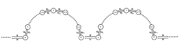
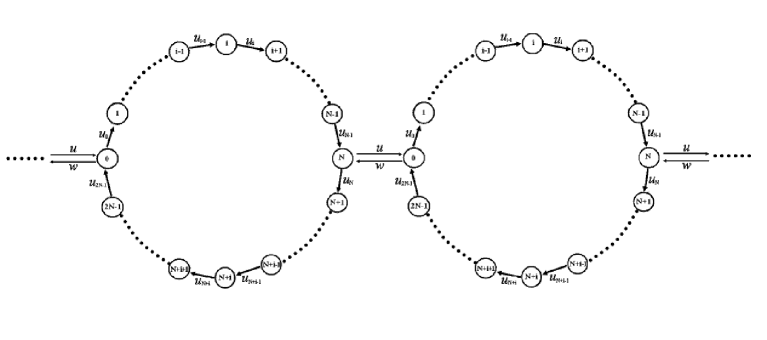
Figure 2: Special cases of the network model: (Up) in which $w_{0}=w_{2N-1}=w_{2N-2}=\cdots=w_{N+1}=0$, and $u_{N}=u_{N+1}=\cdots=u_{2N-1}=0$. (Down) in which $w_{0}=w_{1}=\cdots=w_{2N-1}=0$.

In this case, our network model reduces to the usual one dimensional hopping model [24, 23]. It can be easily found that $J_{i}=\rho_{i-1}u_{i-1}-\rho_{i}w_{i}=0$ for $N+1\leq i\leq 2N$, and $J=\rho_{N}u-\rho_{0}w=\rho_{0}u_{0}-\rho_{1}w_{1}=J_{1}$. By $J_{1}=J_{2}=\cdots=J_{N}$, one obtains

$$\rho_{k}=\rho_{0}\prod_{i=1}^{k}\left(\frac{u_{i-1}}{w_{i}}\right)-\left[1+\sum_{i=1}^{k-1}\prod_{j=i}^{k-1}\left(\frac{u_{j}}{w_{j}}\right)\right]\frac{J}{w_{k}}$$ (19)

and $\rho_{N}=\rho_{0}\prod_{i=1}^{N}\left(\frac{u_{i-1}}{w_{i}}\right)-\left[1+\sum_{i=1}^{N-1}\prod_{j=i}^{N-1}\left(\frac{u_{j}}{w_{j}}\right)\right]\frac{J}{w_{N}}$. At the same time, $\rho_{N}u-\rho_{0}w=J$ implies

$$\frac{J+\rho_{0}w}{u}=\rho_{N}=\rho_{0}\prod_{i=1}^{N}\left(\frac{u_{i-1}}{w_{i}}\right)-\left[1+\sum_{i=1}^{N-1}\prod_{j=i}^{N-1}\left(\frac{u_{j}}{w_{j}}\right)\right]\frac{J}{w_{N}}$$ (20)

which gives

$$\rho_{0}=\frac{1+\left[1+\sum_{i=1}^{N-1}\prod_{j=i}^{N-1}\left(\frac{u_{j}}{w_{j}}\right)\right]\frac{u}{w_{N}}}{u\prod_{i=1}^{N}\left(\frac{u_{i-1}}{w_{i}}\right)-w}J$$ (21)

Combing (19) (21), we get

$$\rho_{k}=\left\{\frac{1+\left[1+\sum_{i=1}^{N-1}\prod_{j=i}^{N-1}\left(\frac{u_{j}}{w_{j}}\right)\right]\frac{u}{w_{N}}}{u\prod_{i=1}^{N}\left(\frac{u_{i-1}}{w_{i}}\right)-w}\prod_{i=1}^{k}\left(\frac{u_{i-1}}{w_{i}}\right)-\left[1+\sum_{i=1}^{k-1}\prod_{j=i}^{k-1}\left(\frac{u_{j}}{w_{j}}\right)\right]\frac{1}{w_{k}}\right\}J$$ (22)

Finally, $\sum_{k=0}^{N}\rho_{k}=1$ gives

$$J=\frac{1}{\bar{A}}$$ (23)

where

$$\bar{A}=\frac{1+\left[1+\sum_{i=1}^{N-1}\prod_{j=i}^{N-1}\left(\frac{u_{j}}{w_{j}}\right)\right]\frac{u}{w_{N}}}{u\prod_{i=1}^{N}\left(\frac{u_{i-1}}{w_{i}}\right)-w}\sum_{k=0}^{N}\left[\prod_{i=1}^{k}\left(\frac{u_{i-1}}{w_{i}}\right)\right]-\sum_{k=0}^{N}\left\{\left[1+\sum_{i=1}^{k-1}\prod_{j=i}^{k-1}\left(\frac{u_{j}}{w_{j}}\right)\right]\frac{1}{w_{k}}\right\}$$ (24)

So in this case, the mean velocity of molecular motors is $V=JL=L/\bar{A}$, and the probabilities $\rho_{k}$ are given by Eqs. (21) (22).

(2) $w_{0}=w_{1}=\cdots=w_{2N-1}=0$ (see Figure 2 (Down)):

In this case, $J_{i}=\rho_{i-1}u_{i-1}$ for $1\leq i\leq 2N$, and $J=\rho_{N}u-\rho_{0}w$. At the steady state

$$\rho_{k}=\frac{u_{0}}{u_{k}}\rho_{0}\qquad\rho_{N+k}=\frac{u_{N}}{u_{N+k}}\rho_{N}\quad\textrm{for}\quad 0\leq k\leq N-1$$ (25)

Due to $J_{N+1}+J=J+{N-1}$, one knows

$$\rho_{N}(u+u_{N})=\rho_{0}(u_{0}+w)$$ (26)

i.e.

$$\rho_{N}=\frac{u_{0}+w}{u+u_{N}}\rho_{0}$$ (27)

in view of (25) (27) and $\sum_{k=0}^{2N-1}\rho_{k}=1$, one obtains

$$\rho_{0}=\frac{1}{u_{0}\sum_{k=0}^{N-1}\frac{1}{u_{k}}+\frac{u_{N}(u_{0}+w)}{u+u_{N}}\sum_{k=N}^{2N-1}\frac{1}{u_{k}}}$$ (28)

hence

$$J= \rho_{N}u-\rho_{0}w=\left(\frac{u(u_{0}+w)}{u+u_{N}}-w\right)\rho_{0}$$ (29)

$$= \frac{uu_{0}-u_{N}w}{u_{0}(u+u_{N})\sum_{k=0}^{N-1}\frac{1}{u_{k}}+u_{N}(u_{0}+w)\sum_{k=N}^{2N-1}\frac{1}{u_{k}}}$$

and the probabilities $\rho_{k}$ can be obtained by Eqs. (25) (27) (28).

(3) $N=1$:

In this case,

$$A=\frac{u_{{1}}+u+w_{{1}}}{w_{0}w_{{1}}}\qquad B=\frac{uu_{{0}}-ww_{{1}}+u_{{0}}u_{{1}}-w_{{1}}w_{{0}}}{w_{{1}}w_{{0}}}$$ (30)

$$C=\left({\frac{uu_{{0}}}{w_{{1}}}}-w\right)\left({\frac{u_{{1}}}{w_{{1}}w_{{0}}}}+{w_{{0}}}^{-1}+{\frac{u}{w_{{1}}w_{{0}}}}\right)\left({\frac{uu_{{0}}}{w_{{1}}w_{{0}}}}-{\frac{w}{w_{{0}}}}+{\frac{u_{{0}}u_{{1}}}{w_{{1}}w_{{0}}}}-1\right)^{-1}-{\frac{u}{w_{{N}}}}$$

$$D=\left({\frac{u_{{1}}}{w_{{1}}w_{{0}}}}+{w_{{0}}}^{-1}+{\frac{u}{w_{{1}}w_{{0}}}}\right)\left({\frac{u_{{0}}}{w_{{1}}}}+1\right)\left({\frac{uu_{{0}}}{w_{{1}}w_{{0}}}}-{\frac{w}{w_{{0}}}}+{\frac{u_{{0}}u_{{1}}}{w_{{1}}w_{{0}}}}-1\right)^{-1}-{w_{{1}}}^{-1}$$

and

$$J=\frac{\frac{\left({\frac{uu_{{0}}}{w_{{1}}}}-w\right)\left({\frac{u_{{1}}}{w_{{1}}w_{{0}}}}+{w_{{0}}}^{-1}+{\frac{u}{w_{{1}}w_{{0}}}}\right)}{{\frac{uu_{{0}}}{w_{{1}}w_{{0}}}}-{\frac{w}{w_{{0}}}}+{\frac{u_{{0}}u_{{1}}}{w_{{1}}w_{{0}}}}-1}-{\frac{u}{w_{{N}}}}}{\frac{\left({\frac{u_{{1}}}{w_{{1}}w_{{0}}}}+{w_{{0}}}^{-1}+{\frac{u}{w_{{1}}w_{{0}}}}\right)\left({\frac{u_{{0}}}{w_{{1}}}}+1\right)}{{\frac{uu_{{0}}}{w_{{1}}w_{{0}}}}-{\frac{w}{w_{{0}}}}+{\frac{u_{{0}}u_{{1}}}{w_{{1}}w_{{0}}}}-1}-\frac{1}{w_{1}}}$$ (31)

The probability flux of the special case (1) is

$$J={\frac{uu_{{0}}-ww_{{1}}}{u_{{0}}+w_{{1}}+u+w}}$$ (32)

The probability flux of the special case (2) is

$$J={\frac{uu_{{0}}-u_{{1}}w}{u+u_{{1}}+u_{{0}}+w}}$$ (33)

(4) $N=2$:

In this case, the probability flux (23) is

$$J={\frac{w_{{1}}w_{{2}}w_{{3}}w_{{0}}}{u_{{1}}u_{{2}}u_{{3}}+u_{{2}}u_{{3}}w_{{1}}+w_{{1}}w_{{2}}w_{{3}}+w_{{1}}w_{{2}}u_{{3}}+uw_{{1}}w_{{3}}+uw_{{1}}u_{{3}}+uu_{{1}}w_{{3}}+uu_{{1}}u_{{3}}}}$$ (34)

the probability flux (29) is

$$J={\frac{\left(uu_{{0}}-u_{{2}}w\right)u_{{1}}u_{{3}}}{uu_{{1}}u_{{3}}+u_{{3}}uu_{{0}}+u_{{1}}u_{{2}}u_{{3}}+u_{{3}}u_{{0}}u_{{2}}+u_{{1}}u_{{0}}u_{{3}}+u_{{1}}u_{{0}}u_{{2}}+u_{{1}}wu_{{3}}+u_{{1}}u_{{2}}w}}$$ (35)

4 The force dependence of the transition rates

As pointed out in the introduction, the transition rates $u_{i},w_{i},u,w$ depend on the external force $F$. For nonzero external force $F$, the force dependence of the transition rates $u_{i},w_{i},u,w$ can be modeled as the following

$$u=k^{+}e^{-\beta\delta FL_{\delta}}\ \ \quad w=k^{-}e^{\beta(1-\delta)FL_{\delta}}$$ (36)

$$u_{i}=k_{i}^{+}e^{-\beta\delta_{i}FL_{i}}\quad w_{i+1}=k_{i+1}^{-}e^{\beta(1-\delta_{i})FL_{i}}\qquad 0\leq i\leq 2N-1$$

where $\beta=1/k_{B}T$, $0\leq\delta,\delta_{i}\leq 1$ are load distribution factors that reflect how the external force affects the individual rates [19, 22, 21] (see Figure 3), $L_{0}+L_{1}+\cdots+L_{N-1}+L_{\delta}=L$, $L_{0}+L_{1}+\cdots+L_{N-1}=L_{N}+L_{N+1}+\cdots+L_{2N-1}$.

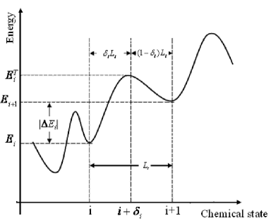
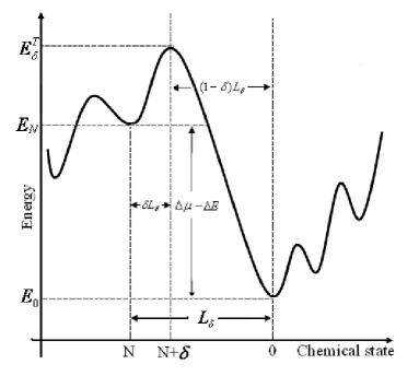
Figure 3: Energy profile of a molecular motor in the neighborhood of local equilibrium mechanochemical state: (Left) Molecular motor undergoes thermal fluctuations around the $i-$th local equilibrium position with potential $E_{i}$, which corresponds to mechanochemical state $i$. It moves forward (to the right) or backward (to the left) when it acquires enough energy to across the energy barriers $E^{T}_{i}$ or $E^{T}_{i-1}$. The local equilibrium position $i$ and $i+1$ are separated by characteristic distance $L_{i}$, the local equilibrium state $i$ and the transition state ${i+\delta_{i}}$ with energy $E^{T}_{i}$ are separated by characteristic distance $\delta_{i}L_{i}$, and the local equilibrium state $i+1$ and the transition state ${i+\delta_{i}}$ are separated by characteristic distance $(1-\delta_{i})L_{i}$. The energy difference between state $i$ and $i+1$ is $\triangle E_{i}=E_{i}-E_{i+1}$. (Right) Molecular motor undergoes thermal fluctuations around the $N-$th local equilibrium position with potential $E_{N}$, which corresponds to mechanochemical state $N$. It moves forward (to the right) when it acquires enough energy to across the energy barriers $E^{T}_{\delta}$. The local equilibrium $N$ and $0$ are separated by characteristic distance $L_{\delta}$, the local equilibrium $N$ and the transition state $N+\delta$ with energy $E^{T}_{\delta}$ are separated by characteristic distance $\delta L_{\delta}$, the local equilibrium $0$ and the transition state $N+\delta$ are separated by characteristic distance $(1-\delta)L_{\delta}$. The energy difference between state $0$ and $N$ is $\triangle\mu-\triangle E$.

In (36), the load distribution factors $\delta$ and $\delta_{i}$ can be determined by experimental data as in [25, 26, 27, 28]. Thermodynamic consistency requires $k_{i}^{+}/k_{i+1}^{-}=e^{\beta\triangle E_{i}}$ and $k^{+}/k^{-}=e^{\beta(\triangle\mu-\triangle E)}$, where $\triangle E_{i}=E_{i}-E_{i+1}$ is the potential energy difference between mechanochemical states $i$ and $i+1$ (see Figure 3), $\triangle E=\sum_{i=0}^{N-1}\triangle E_{i}=E_{0}-E_{N}$ is the potential energy difference between mechanochemical states $0$ and state $N$, in the no external force case, which is the energy barrier of the movement of molecular motors. $\triangle\mu$ is the chemical energy transferred to the motors in one mechachemical step, which comes from the hydrolysis of the fuel molecule ATP (see Figure 4).

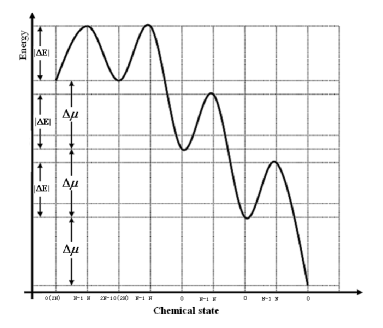
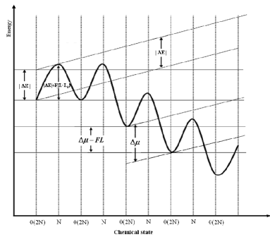
Figure 4: The energy profile in mechanochemical cycles: (Left) No external force case: the energy barrier between mechanochemical states $0$ and $N$ is $|\triangle E|$. After mechanochemical state $N$, the molecular motor might back to state $0$ through mechanochemical passway $N\to N-1\to\cdots\to 0$ or $N\to N+1\to\cdots\to 2N(0)$. In this case, the molecular motor makes no any mechanical steps. Also, the molecular motor might back to state $0$ immediately through mechanochemical passway $N\to 0$. In such case, molecular motor completes one forward mechanical step, with one fuel molecule ATP is hydrolyzed. The free energy released by one ATP molecule is $\triangle\mu$. (Right) Nonzero external force $F$ case: in this case, the energy barrier between mechanochemical states $0$ and $N$ is $|\triangle E|+F(L-L_{\delta})$, which is bigger than the no external force case. So it will be more difficult for molecular motors to make a forward step. During one forward step, the energy dissipation is $\triangle\mu-FL$, which is small than the no external force case, since part of the energy $\triangle\mu$ released by the ATP is used to do useful mechanical work.

5 Continuous mechanochemical state multi-cycle network model

As the number of mechanochemical states $2N$ tends to infinite, our multi-cycle network model (see Figure 1) can be approximated by the continuous mechanochemical state model (see Figure 5).

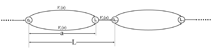
Figure 5: Depiction of continuous mechanochemical state multi-cycle network model: There’re two chemical passway between mechanochemical state $0_{k}$ and $1_{k}$, in which the potentials are $V_{1}(x)$ and $V_{2}(x)$ ($kL\leq x\leq kL+a$) respectively. The potential between mechanochemical state $1_{k}$ and $0_{k+1}$ is $V_{3}(x)$ ($kL+a\leq x\leq(k+1)L$).

In this model, there’re two chemical passway from state $0_{k}$ to state $1_{k}$ with different potentials $V_{1}(x)$ and $V_{2}(x)$ ($kL\leq x\leq kL+a$) respectively. From state $1_{k}$ to state $0_{k+1}$, the potential function is $V_{3}(x)$ ($kL+a\leq x\leq(k+1)L$). Biophysically, the potentials $V_{i}(x)$ are periodical, i.e $V_{i}(x+L)=V(x)$, and satisfy $V_{1}(0_{k})=V_{2}(0_{k}),V_{1}(1_{k})=V_{2}(1_{k})=V_{3}(1_{k})$.

In the $i-$th chemical passway, the motion of molecular motors can be described by the following Fokker-Planck equation:

$$\frac{\tilde{\rho}_{i}(x,t)}{\partial t}=\frac{\partial}{\partial x}\left(\frac{\tilde{\rho}_{i}(x,t)}{\gamma}\frac{\partial V_{i}(x)}{\partial x}+D\frac{\partial\tilde{\rho}_{i}(x,t)}{\partial x}\right)=-\frac{\partial\tilde{J}_{i}}{\partial x}$$ (37)

$$\textrm{where}\qquad kL\leq x\leq kL+a\qquad\qquad\ \textrm{for}\quad i=1,2$$

$$\qquad\qquad\ \ kL+a\leq x\leq(k+1)L\qquad\textrm{for}\quad i=3$$

in which $\gamma$ is viscous friction coefficient, $D$ is free diffusion coefficient which satisfies Einstein relation $D=k_{B}T/\gamma$, $\tilde{\rho}_{i}(x,t)$ is probability density for finding molecular motors at mechanochemical state $x$ in $i-$th passway at time $t$ and $\tilde{J}_{i}(x,t)$ is the probability flux. Define

$$\rho_{i}(x,t)=\sum_{k=-\infty}^{\infty}\tilde{\rho}_{i}(x+kL,t)\qquad J_{i}(x,t)=\sum_{k=-\infty}^{\infty}\tilde{J}_{i}(x+kL,t)$$ (38)

it can be readily verified that

$$\frac{\rho_{i}(x,t)}{\partial t}=\frac{\partial}{\partial x}\left(\frac{\rho_{i}(x,t)}{\gamma}\frac{\partial V_{i}(x)}{\partial x}+D\frac{\partial\rho_{i}(x,t)}{\partial x}\right)=-\frac{\partial J_{i}}{\partial x}$$ (39)

$$\textrm{where}\qquad 0\leq x\leq a\qquad\textrm{for}\quad i=1,2$$

$$\qquad\qquad\ a\leq x\leq L\qquad\textrm{for}\quad i=3$$

At steady state, the probability flux $J_{i}$ is constant and the probability $\rho_{i}(x)$ satisfies

$$\frac{\partial\rho_{i}(x,t)}{\partial x}+\frac{\partial V_{i}(x)}{\partial x}\frac{\rho_{i}(x,t)}{k_{B}T}=-\frac{J_{i}}{D}$$ (40)

$$\textrm{where}\qquad 0\leq x\leq a\qquad\textrm{for}\quad i=1,2$$

$$\qquad\qquad\ a\leq x\leq L\qquad\textrm{for}\quad i=3$$

Under the following constraints

$$\int_{0}^{a}\rho_{1}(x)dx+\int_{0}^{a}\rho_{2}(x)dx+\int_{a}^{b}\rho_{3}(x)dx=1$$ (41)

$$\rho_{1}(0)=\rho_{2}(0)=\rho_{3}(L)\quad\rho_{1}(a)=\rho_{2}(a)=\rho_{3}(a)\quad J_{1}+J_{2}=J_{3}$$

we can get the solutions of (40)

$$\rho_{i}(x)=\left(C_{i}-\frac{J_{i}}{D}\int_{0}^{x}e^{\frac{V_{i}(y)}{k_{B}T}}dy\right)e^{-\frac{V_{i}(x)}{k_{B}T}}\quad\textrm{for}\ \ i=1,2$$ (42)

$$\rho_{3}(x)=\left(C_{3}-\frac{J_{3}}{D}\int_{a}^{x}e^{\frac{V_{3}(y)}{k_{B}T}}dy\right)e^{-\frac{V_{3}(x)}{k_{B}T}}$$

where the constants $C_{1},C_{2},C_{3}$ are the following

$$C_{1}=C_{2}=\frac{\left[\int_{0}^{a}\left(e^{\frac{V_{1}(y)}{k_{B}T}}+e^{\frac{V_{2}(y)}{k_{B}T}}\right)dy\right]\left(\int_{a}^{L}e^{\frac{V_{3}(y)}{k_{B}T}}dy\right)+\left(\int_{0}^{a}e^{\frac{V_{1}(y)}{k_{B}T}}dy\right)\left(\int_{0}^{a}e^{\frac{V_{2}(y)}{k_{B}T}}dy\right)}{e^{\frac{V_{3}(L)-V_{1}(0)}{k_{B}T}}\Delta}$$

$$C_{3}=\frac{\left[\int_{0}^{a}\left(e^{\frac{V_{1}(y)}{k_{B}T}}+e^{\frac{V_{2}(y)}{k_{B}T}}\right)dy\right]\left(\int_{a}^{L}e^{\frac{V_{3}(y)}{k_{B}T}}dy\right)e^{\frac{V_{1}(0)-V_{3}(L)}{k_{B}T}}+\left(\int_{0}^{a}e^{\frac{V_{1}(y)}{k_{B}T}}dy\right)\left(\int_{0}^{a}e^{\frac{V_{2}(y)}{k_{B}T}}dy\right)}{\Delta}$$

and the probability fluxes $J_{1},J_{2},J_{3}$ are

$$J_{1}=\left.\left(e^{\frac{V_{1}(0)-V_{3}(L)}{k_{B}T}}-1\right)\left(\int_{0}^{a}e^{\frac{V_{2}(y)}{k_{B}T}}dy\right)D\right/\Delta$$ (43)

$$J_{2}=\left.\left(e^{\frac{V_{2}(0)-V_{3}(L)}{k_{B}T}}-1\right)\left(\int_{0}^{a}e^{\frac{V_{1}(y)}{k_{B}T}}dy\right)D\right/\Delta$$

$$J_{3}=J_{1}+J_{2}$$

The expression $\Delta$ is

$$\Delta= \left[\left(\int_{0}^{a}e^{\frac{V_{1}(y)}{k_{B}T}}dy\right)\left(\int_{0}^{a}e^{\frac{V_{2}(y)}{k_{B}T}}dy\right)+\left(\int_{0}^{a}e^{\frac{V_{2}(y)}{k_{B}T}}dy\right)\left(\int_{a}^{L}e^{\frac{V_{3}(y)}{k_{B}T}}dy\right)\right.$$

$$+\left.\left(\int_{0}^{a}e^{\frac{V_{1}(y)}{k_{B}T}}dy\right)\left(\int_{a}^{L}e^{\frac{V_{3}(y)}{k_{B}T}}dy\right)\right]$$

$$\times\left[\int_{0}^{a}e^{-\frac{V_{1}(y)}{k_{B}T}}dy+\int_{0}^{a}e^{-\frac{V_{2}(y)}{k_{B}T}}dy+\int_{a}^{L}e^{-\frac{V_{3}(y)}{k_{B}T}}dy\right]e^{\frac{V_{1}(0)-V_{3}(L)}{k_{B}T}}$$

$$+\left[\left(\int_{0}^{a}e^{\frac{V_{1}(y)}{k_{B}T}}dy\right)\left(\int_{0}^{a}e^{\frac{V_{2}(y)}{k_{B}T}}dy\right)\left(\int_{a}^{L}e^{-\frac{V_{3}(y)}{k_{B}T}}dy\right)\right.$$

$$+\left.\left(\int_{0}^{a}\int_{0}^{x}e^{\frac{V_{2}(y)-V_{2}(x)}{k_{B}T}}dydx+\int_{a}^{L}\int_{a}^{x}e^{\frac{V_{3}(y)-V_{3}(x)}{k_{B}T}}dydx\right)\left(\int_{0}^{a}e^{\frac{V_{1}(y)}{k_{B}T}}dy\right)\right.$$

$$+\left.\left(\int_{0}^{a}\int_{0}^{x}e^{\frac{V_{1}(y)-V_{1}(x)}{k_{B}T}}dydx+\int_{a}^{L}\int_{a}^{x}e^{\frac{V_{3}(y)-V_{3}(x)}{k_{B}T}}dydx\right)\left(\int_{0}^{a}e^{\frac{V_{2}(y)}{k_{B}T}}dy\right)\right]$$

$$\times\left(1-e^{\frac{V_{1}(0)-V_{3}(L)}{k_{B}T}}\right)$$

$$= \left(\int_{0}^{a}e^{\frac{V_{1}(y)}{k_{B}T}}dy\right)\left(\int_{0}^{a}e^{\frac{V_{2}(y)}{k_{B}T}}dy\right)\left(\int_{a}^{L}e^{-\frac{V_{3}(y)}{k_{B}T}}dy\right)$$

$$+\left(\int_{0}^{a}\int_{0}^{x}e^{\frac{V_{2}(y)-V_{2}(x)}{k_{B}T}}dydx+\int_{a}^{L}\int_{a}^{x}e^{\frac{V_{3}(y)-V_{3}(x)}{k_{B}T}}dydx\right)\left(\int_{0}^{a}e^{\frac{V_{1}(y)}{k_{B}T}}dy\right)$$

$$+\left(\int_{0}^{a}\int_{0}^{x}e^{\frac{V_{1}(y)-V_{1}(x)}{k_{B}T}}dydx+\int_{a}^{L}\int_{a}^{x}e^{\frac{V_{3}(y)-V_{3}(x)}{k_{B}T}}dydx\right)\left(\int_{0}^{a}e^{\frac{V_{2}(y)}{k_{B}T}}dy\right)$$

$$+\left\{\left(\int_{0}^{a}\int_{x}^{a}e^{\frac{V_{2}(y)-V_{2}(x)}{k_{B}T}}dydx+\int_{a}^{L}\int_{x}^{L}e^{\frac{V_{3}(y)-V_{3}(x)}{k_{B}T}}dydx\right)\left(\int_{0}^{a}e^{\frac{V_{1}(y)}{k_{B}T}}dy\right)\right.$$

$$+\left(\int_{0}^{a}\int_{x}^{a}e^{\frac{V_{1}(y)-V_{1}(x)}{k_{B}T}}dydx+\int_{a}^{L}\int_{x}^{L}e^{\frac{V_{3}(y)-V_{3}(x)}{k_{B}T}}dydx\right)\left(\int_{0}^{a}e^{\frac{V_{2}(y)}{k_{B}T}}dy\right)$$

$$+\left[\left(\int_{0}^{a}e^{\frac{V_{2}(y)}{k_{B}T}}dy\right)\left(\int_{a}^{L}e^{\frac{V_{3}(y)}{k_{B}T}}dy\right)+\left(\int_{0}^{a}e^{\frac{V_{1}(y)}{k_{B}T}}dy\right)\left(\int_{a}^{L}e^{\frac{V_{3}(y)}{k_{B}T}}dy\right)\right]$$

$$\times\left.\left[\int_{0}^{a}e^{-\frac{V_{1}(y)}{k_{B}T}}dy+\int_{0}^{a}e^{-\frac{V_{2}(y)}{k_{B}T}}dy\right]\right\}e^{\frac{V_{1}(0)-V_{3}(L)}{k_{B}T}}$$

$$> 0$$

Therefore, in the framework of this continuous mechanochemical state multi-cycle network model, the expression of the mean velocity of molecular motors is

$$V=(J_{1}+J_{2})a+J_{3}(L-a)=\frac{\left(e^{\frac{V_{1}(0)-V_{3}(L)}{k_{B}T}}-1\right)\left[\int_{0}^{a}\left(e^{\frac{V_{1}(y)}{k_{B}T}}+e^{\frac{V_{2}(y)}{k_{B}T}}\right)dy\right]DL}{\Delta}$$ (44)

Obviously, $V>0$ if $V_{1}(0)>V_{3}(L)$ and $V<0$ if $V_{1}(0)<V_{3}(L)$. It can be readily verified that the equations (1) (2) can be obtained by applying spatial discretization to Fokker-Planck equation (37), with some detailed expression of the transition rate $u_{i},w_{i}$ (see [29]).

6 Concluding remarks

In this paper, a general multi-cycle network model of molecular motors is theoretically discussed. The explicit formulation of the velocity has been obtained. This model can be regarded as a generalization of the one designed by Liepelt and Lipowsky in [18] and the one used by T. Schmiedl and U. Seifert in [19]. The method used in this paper is similar as the methods used by Derrida, Fisher and Kolomeisky [22, 23, 24].

Acknowledgments

This work was funded by National Natural Science Foundation of China (Grant No. 10701029).

References

• [1] DavidΒ D. Hackney. Processive motor movement. Science, 316:58–59, 2007.
• [2] N.Β J. Carter and R.Β A. Cross. Mechanics of the kinesin step. Nature, 435:308–312, 2005.
• [3] Y.Β Taniguchi, M.Β Nishiyama, Y.Β Ishhi, and T.Β Yanagida. Entropy rectifies the brownian step of kinesin. Nature Chemical Biology, 1:342–347, 2005.
• [4] R.Β D. Vale. The molecular motor toolbox for intracellular transport. Cell, 112:467–480, 2003.
• [5] H.Β Sakakibara, H.Β Kojima, Y.Β Sakai, E.Β Katayama, and K.Β Oiwa. Inner-arm dynein c of chlamydomonas flagella is a single-headed processive motor. Nature, 400:596–589, 1999.
• [6] A.Β M. Hooft, E.Β J. Maki, K.Β K. Cox, and J.Β E. Baker. An accelerated state of myosin-based actin motility. Biochemistry, 46:3513–3520, 2007.
• [7] J.Β Christof, M.Β Gebhardt, Anabel E.-M. Clemen, Johann Jaud, and Matthias Rief. Myosin-v is a mechanical ratchet. PNAS, 103:8680–8685, 2006.
• [8] Katsuyuki Shiroguchi and KazuhikoΒ Kinosita Jr. Myosin v walks by lever brownian motion. Science, 316:1208–1212, 2007.
• [9] H.Β Noji, R.Β Yasuda, M.Β Yoshida, and Jr.Β K. Kinosita. Direct observation of the rotation of f1-atpase. Nature, 386:299–302, 1997.
• [10] J.Β Howard. Mechanics of Motor Proteins and the Cytoskeleton. Sinauer Associates, Sunderland, MA, 2001.
• [11] Yunxin Zhang. The efficiency of molecular motors. Journal of Statistical Physics, 134:669–679, 2009.
• [12] K.Β Svoboda and S.M. Block. Force and velocity measured for single kinesin molecules. Cell, 77:773–784, 1994.
• [13] Frank JΓΌlicher, Armand Ajdari, and Jacques Prost. Modeling molecular motors. Reviews of Modern Physics, 69(4):1269–1281, 1997.
• [14] Hong Qian. Cycle kinetics, steady state thermodynamics and motors a paradigm for living matter physics. Journal of Physics: Condensed Matter, 17:S3783–S3794, 2005.
• [15] AnatolyΒ B. Kolomeisky and MichaelΒ E. Fisher. Molecular motors: A theorist s perspective. Annual Review of Physical Chemistry, 58:675–695, 2007.
• [16] Hong Qian. A simple theory of motor protein kinetics and energetics. Biophysical Chemistry, 67:263–267, 1997.
• [17] Steffen Liepelt and Reinhard Lipowsky. Kinesin s network of chemomechanical motor cycles. Physical Review Letters, 98(25):258102, 2007.
• [18] Steffen Liepelt and Reinhard Lipowsky. Operation modes of the molecular motor kinesin. Physical Review E, 79(1):011917, 2009.
• [19] T.Β Schmiedl and U.Β Seifert. Efficiency of molecular motors at maximum power. Europhysics Letters, 83:30005, 2008.
• [20] Field Cady and Hong Qian. Open-system thermodynamic analysis of DNA polymerase fidelity. Preprint, 2009.
• [21] A.Β W.Β C. Lau, D.Β Lacoste, and K.Β Mallick. Nonequilibrium fluctuations and mechanochemical couplings of a molecular motor. Physical Review Letters, 99:158102, 2007.
• [22] MichaelΒ E. Fisher and AnatolyΒ B. Kolomeisky. Simple mechanochemistry describes the dynamics of kinesin molecules. Proceedings of the National Academy of Sciences, 98(14):7748–7753, 2001.
• [23] AnatolyΒ B. Kolomeisky and MichaelΒ E. Fisher. Periodic sequential kinetic models with jumping, branching and deaths. Physica A, 279:1–20, 2000.
• [24] Bernard Derrida. Velocity and diffusion constant of a periodic one-dimensional hopping model. Journal of Statistical Physics, 31(3):433–450, 1983.
• [25] Masayoshi Nishiyama, Hideo Higuchi, and Toshio Yanagida. Chemomechanical coupling of the forward and backward steps of single kinesin molecules. Nature Cell Biology, 4:790–797, 2002.
• [26] Masayoshi Nishiyama, Hideo Higuchi, Yoshiharu Ishii, Yuichi Taniguchi, and Toshio Yanagida. Single molecule processes on the stepwise movement of atp-driven molecular motors. BioSystems, 71:145–156, 2003.
• [27] Yuichi Taniguchi, Masayoshi Nishiyama, Yoshiharu Ishhi, and Toshio Yanagida. Entropy rectifies the brownian step of kinesin. Nature Chemical Biology, 1:342–347, 2005.
• [28] Yunxin Zhang. Three phase model of the processive motor protein kinesin. Biophysical Chemistry, 136:19–22, 2008.
• [29] Hongyun Wang, CharlesΒ S. Peskin, and TimothyΒ C. Elston. A robust numerical algorithm for studying biomolecular transport processes. Journal of Theoretical Biology, 221:491–511, 2003.