Kinematics of the Outer Pseudorings and the Spiral Structure of the Galaxy

Abstract

The kinematics of the outer rings and pseudorings is determined by two processes: the resonance tuning and the gas outflow. The resonance kinematics is clearly observed in the pure rings, while the kinematics of the gas outflow is manifested itself in the pseudorings. The direction of systematical motions in the pure rings depends on the position angle of a point with respect to the bar major axis and on the class of the outer ring. The direction of the radial and azimuthal components of the residual velocities of young stars in the Perseus, Carina, and Sagittarius regions can be explained by the presence of the outer pseudoring of class $R_{1}R_{2}^{\prime}$ in the Galaxy. We present models, which reproduce the directions and values of the residual velocities of OB-associations in the Perseus and Sagittarius regions, and also model reproducing the directions of the residual velocities in the Perseus, Sagittarius, and Carina regions. The kinematics of the Sagittarius region accurately defines the solar position angle with respect to the bar elongation, $\theta_{b}=45\pm 5^{\circ}$.

20093500001[000]

November 11, 2008; in final form, February 04, 2009

1 INTRODUCTION

1.1 The Galactic spiral structure

Figure 1: (a) The residual velocities of OB-associations projected onto the galactic plane. The union of OB-associations into regions of intense star formation. (b) The average velocities, $V_{R}$ and $V_{\theta}$, of OB-associations in the regions of intense star formation. The X-axis is directed away from the center, the Y-axis is in the direction of the Galactic rotation. The Sun is at the origin.

The spiral structure is clearly observed in many external galaxies viewed face-on, but in the Galaxy we are faced with a difficulty of the distance determination for the indicators of spiral structure. On the other hand, in the Galaxy we can study the field of space velocities using both line-of-sight velocities and proper motions, whereas with other galaxies we are almost completely limited to line-of-sight velocities.

One of the best tracers of the spiral structure are HII regions – gas clouds which are ionized by young hot stars. These can be seen as bright radio objects throughout the disc of the Galaxy (Georgelin and Georgelin 1976; Russeil 2003; and other papers). Though the distances for the distant HII regions, $r>4$ kpc, are determined from observations badly (usually they are derived from the kinematical models) the distribution of HII regions displays the most general features of the Galactic spiral structure which can be formulated as follows.

• The Galactic spiral structure is most pronounced at the Galactocentric distances $R=5-9$ kpc.

• The pitch angle of the Galactic spirals is quite small, $i<20^{\circ}$.

• Many researchers believe the Galaxy is 4-armed.

In the vicinity of 3 kpc from the Sun the optical data has revealed the existence of three fragments of the spiral structure: Sagittarius-Carina, Cygnus-Orion, and Perseus ones. The characteristic of these regions is the intense star formation manifested as increased concentration of young clusters and OB-associations (Humphreys 1979; and other papers)

The Sagittarius-Carina and Perseus arm-fragments are often thought to be part of the global spiral structure (Georgelin and Georgelin 1976; Efremov 1998; Russeil 2003; Vallée 2005; and other papers). The Cygnus-Orion fragment is usually regarded as the local arm. This conception appears mostly because of its location between two global arms.

The study of the Galactic structure in the neutral hydrogen revealed the existence of regions with systematical non-circular motions which were later identified with spiral arms (Burton 1971). The investigation of the Perseus region in OB-associations, red supergiants, molecular and neutral hydrogen showed the presence of systematical motions which were interpreted as motions directed towards the Galactic center (Burton and Bania 1974; Humphreys 1976; Avedisova and Palous 1989; Brand and Blitz 1993; and other papers). Recent studies agree with this result (Melnik et al. 2001; Sitnik 2003; and other papers).

The density-wave theory which had been already developed by the end of the 60s (Lin et al. 1969, Lin 1970; Roberts 1969) afforded an opportunity to determine the location of spiral arms with respect to the corotation radius (CR) through the direction of gas streaming motions in spiral arms. The direction of streaming motions in the Perseus region strongly suggests that its location is inside the CR.

The density-wave theory describes the kinematics of young stars and gas in the Perseus, Cygnus, and Carina regions quite well (Melnik 2003). Nevertheless its application to the whole 3-kpc solar neighborhood encounters some difficulties. Young stars in the Carina and Sagittarius regions, through which the spiral arm is traditionally drawn, have different systematical motions and cannot be fragments of the same density-wave spiral arm. Moreover, the young stars with the systematical non-circular motions directed towards the Galactic center (the Perseus, Cygnus, and Carina regions) which could belong to the same, perhaps patchy, spiral arm fall nicely on a large-scale structure which appears to be the leading spiral arm (Melnik 2006).

In the present paper we intend to build the dynamical models that reproduce the kinematics of young stars in the 3-kpc solar neighborhood. We’ll show that model of the Galaxy with an outer ring of class $R_{1}R_{2}^{\prime}$ can explain the kinematics of young stars in some regions.

1.2 The kinematics of young stars within 3 kpc of the Sun

Table 1: Average residual velocities of OB-associations

Region	R, kpc	$V_{R}$,	$V_{\theta}$,	l, deg.	r, kpc	Associations
		km s-1	km s-1
Sagittarius	5.6	$+11\pm 3$	$-1\pm 1$	8–23	1.3–1.9	Sgr OB1, OB7, OB4, Ser OB1, OB2,
						Sct OB2, OB3;
Carina	6.5	$-6\pm 2$	$+5\pm 3$	286–315	1.5–2.1	Car OB1, OB2, Cru OB1, Cen OB1,
						Coll 228, Tr 16, Hogg 16, NGC 3766, 5606;
Cygnus	6.9	$-7\pm 3$	$-11\pm 2$	73–78	1.0–1.8	Cyg OB1, OB3, OB8, OB9;
Local System	7.4	$+5\pm 3$	$+0\pm 3$	0–360	0.1–0.6	Per OB2, Mon OB1, Ori OB1, Vela OB2,
						Coll 121, 140, Sco OB2;
Perseus	8.4	$-7\pm 2$	$-5\pm 2$	104–135	1.8–2.8	Per OB1, NGC 457, Cas OB8, OB7, OB6,
						OB5, OB4, OB2, OB1, Cep OB1;

OB-associations are the most suitable objects for the kinematical investigations in the wide solar neighborhood. These loose groups of high-luminosity stars have quite reliable distances (the average accuracy is about 15%). This good accuracy appears due to young clusters which often enter OB-associations (Garmany and Stencel 1992). But unlike young clusters OB-associations contain a sufficient number of stars with known line-of-sight velocities and proper motions. On average the space velocities of OB-associations are determined over 11 stars. The stellar proper motions were taken from the Hipparcos catalog (1997). The electronic version of the catalog of line-of-sight velocities and proper motions of OB-associations is available at http://lnfm1.sai.msu.ru/$\sim$anna/page3.html (for more details, see Melnik et al. 2001).

Fig. 1a shows the residual velocities of OB-associations in a projection onto the Galactic plane. The residual velocities were calculated as the differences between the observed heliocentric velocities and the velocities due to the circular rotation law and the solar motion relative to the centroid of OB-associations. The parameters of the circular Galactic rotation law and the components of the solar motion were derived from the sample of OB-associations located within 3 kpc from the Sun (Melnik et al. 2001). In such a large region systematical non-circular motions of OB-associations can be regarded as random deviations from the rotation curve. The obtained parameters describe the rotation of the low-dispersed Galactic subsystem. Calculation of the residual velocities with respect to the rotation curve derived from the same objects yields minimal residual velocities, any other rotation curve would produce larger, on average, deviations. Besides, the use of the self-consistent distance scale also decreases the deviations from the rotation curve (Sitnik and Melnik 1996; Dambis et al. 2001). The derived rotation curve is nearly flat and corresponds to the linear velocity at the solar distance $\Theta_{0}=215$ km s^-1, the value of $\Theta$ remains constant inside 3 kpc from the Sun with the accuracy $\pm 3$%. We adopted the Galactocentric distance of the Sun to be $R_{0}=7.1$ kpc (Dambis at al. 1995; Glushkova et al. 1998; and other papers). The distances for OB-associations from the catalog by Blaha and Humphreys (1989) were multiplied by a factor of $0.8$ to be consistent with the so-called short distance scale for classical Cepheids (Berdnikov et al. 2000).

Fig. 1a also shows the union of OB-associations into regions of intense star formation which practically coincide with the stellar-gas complexes united by Efremov and Sitnik (1988). Fig. 1b represents the average residual velocities of OB-associations in regions of intense star formation in projection onto the radial, $V_{R}$, and azimuthal, $V_{\theta}$, directions. It is a generalization of Fig. 1a. The average residual velocities and their random errors are given in Table 1, which also contains the average Galactocentric distances $R$, the intervals of galactic longitudes $l$, the intervals of heliocentric distances $r$, and names of OB-association the region includes.

The study of the Hipparcos catalog (1997) shows that systematical errors in positions of bright stars ($m<9^{m}$) don’t exceed 0.0001 arcsec (Kovalevsky, 2002). Stars of the Blaha and Humphreys’ catalog (1989) having the known proper motion are bright enough, their average magnitude equals $m_{V}=7.3^{m}$ in the region $0<r<3$ kpc and $m_{V}=7.8^{m}$ in the region $1.5<r<3$ kpc. Since the mission of Hipparcos (1997) continued several years (37 months), we can suppose that systematical errors of proper motions of stars of OB-associations don’t exceed 0.0001 arcsec yr^-1, that corresponds to the velocity of 1 km s^-1 at the distance of $r=2$ kpc. Besides, the contribution of systematical errors decreases after averaging of proper motions over a large area: most of OB-associations occupy on the sky more than 10 square degrees.

The velocity $V_{R}$ in the Perseus, Cygnus and Carina regions is directed towards the Galactic center and is about $V_{R}=-7$ km s^-1. In the Sagittarius region it is directed away from the Galactic center, $V_{R}=+11$ km s^-1. This means that Sagittarius and Carina regions cannot belong to the same trailing density-wave spiral arm. The Carina region has kinematics typical for a spiral arm inside the CR, whereas the Sagittarius region has kinematics typical for its being outside the CR. However, their kinematics contradicts their location: the Sagittarius region ($R=5.6$ kpc) is located closer to the Galactic center than the Carina region ($R=6.5$ kpc). Thus, the simple trailing density-wave spiral arm is not applicable to the Galaxy.

The velocity $V_{\theta}$ is conspicuous only in the Carina, Cygnus, and Perseus regions. In the Carina region the velocity $V_{\theta}$ is directed in the sense of Galactic rotation ($V_{\theta}=+5$ km s^-1), while in the Perseus ($V_{\theta}=-5$ km s^-1) and Cygnus ($V_{\theta}=-11$ km s^-1) regions it is in the opposite sense.

1.3 Morphology and modelling of the outer pseudorings

The essential characteristic of the galaxies with the outer rings and pseudorings – incomplete rings made up of spiral arms – is the presence of the bar (Buta 1995; Buta and Combes 1996). Two main classes of the outer rings and pseudorings have been identified: the $R_{1}$ rings ($R^{\prime}_{1}$ pseudorings) elongated perpendicular to the bar and the $R_{2}$ rings ($R^{\prime}_{2}$ pseudorings) elongated parallel to the bar. In addition, there is a combined morphological type $R_{1}R_{2}^{\prime}$ which shows elements of both classes. The $R_{2}$ rings have elliptical shape, but the $R_{1}$ rings are often “dimpled” near the bar ends. There is also a lot of outer rings/pseudorings that cannot be classified into previous classes because their morphological characteristics are unclear or the inclination prevents detailed classification (Buta 1995; Buta and Crocker 1991; Buta et al. 2007).

The outer rings are typically observed in early-type galaxies. For the galaxies in the lower red-shift range the frequency of the outer rings is found to be about 10% of all types of spiral galaxies. But for the early-type sample it increases to 20% (Buta and Combes 1996). A study by Buta (1995) shows the following distribution among the main outer ring types: 18% ($R_{1}$), 37% ($R_{1}^{\prime}$), under 1% ($R_{2}$), 35% ($R_{2}^{\prime}$), and 9% ($R_{1}R_{2}^{\prime}$). The small fraction of the complete $R_{2}$ rings may be due to the selection effects – they lack conspicuous features, for example, ”dimples”, and so their definite classification can be difficult due to orientation uncertainties.

The test particle simulations (Schwarz 1981; Byrd et al. 1994; Rautiainen and Salo 1999) and N-body simulations (Rautiainen and Salo 2000) show that the outer pseudorings are typically located in the region of the Outer Lindblad Resonance (OLR) and are connected with two main families of periodic orbits. Main families of stable periodic orbits are followed by most non-periodic orbits after the introduction of the bar potential (Contopoulos and Papayannopulos 1980). The $R_{1}$ rings are supported by periodic orbits lying inside the OLR and elongated perpendicular to the bar, while the $R_{2}$ rings are supported by orbits situated outside the OLR and elongated along the bar.

As convincingly shown by Schwarz (1981) the pseudorings appear before the pure rings. According to Schwarz (1981, 1984), the type of an outer ring is determined by two factors: the bar’s strength and the initial distribution of gas particles. Under the stronger bar forcing the pure $R_{1}$ ring no longer forms, instead, particles move outside through the OLR and form the pseudoring $R_{2}^{\prime}$. However, this idea contradicts observations: the $R_{2}^{\prime}$ pseudorings are more frequently observed in SAB galaxies than in SB ones (Buta 1995).

Simulations demonstrate that such factors as the strong bar, a large radius of the initial particle distribution, and a large model time favor the formation of the $R_{2}$ component. Byrd et al. (1994) find that the $R_{1}$ component appears quickly and the $R_{2}$ component forms slower. All their models yield the $R_{1}^{\prime}$ pseudoring at the earlier time and the $R_{2}^{\prime}$ or the combined $R_{1}R_{2}^{\prime}$ pseudoring at the later time.

In some galaxies with the combined morphology the $R_{1}$ component can be seen in infrared, but the $R_{2}^{\prime}$ component is usually prominent only in blue. Byrd et al. (1994) explain this fact by the age difference between two components. N-body simulations suggest another explanation. Rautiainen and Salo (2000) think that at least some stellar $R_{1}^{\prime}$ rings are not remnants of previous ring-shaped star formation episode, but forms due to self-gravity in the stellar subsystem.

Galactic disks in some simulations demonstrate the presence of the slow modes near the radius of the outer ring (Rautiainen and Salo 1999, 2000). We like to emphasize that the present paper explains the kinematics of young stars without invoking the slow modes.

1.4 The bar, rotation curve, and a prototype of the Galaxy

Our Galaxy certainly has the bar. The gas kinematics in the central region, infrared photometry, star counts, and other modern tests confirm this fact (Weiner and Sellwood, 1999; Benjamin et al. 2005; Englmaier and Gerhard 2006; Habing et al. 2006; Cabrera-Lavers et al. 2007; and other papers). There is ample evidence suggesting that the major axis of the bar is oriented in the direction $\theta_{b}=15\textrm{--}45^{\circ}$ in such a way that the end of the bar closest to the Sun lies in the first quadrant. However, the angular speed of the bar $\Omega_{b}$ and its length are determined from observations badly. Some researchers believe that the CR of the bar lies at the distance range $R=3\textrm{--}4$ kpc (Englmaier and Gerhard 2006; Habing et al. 2006; and references therein), whereas others suggest that the Galaxy has a longer bar with the major axis of $a=4\textrm{--}5$ kpc (Weiner and Sellwood, 1999; Benjamin et al. 2005; Cabrera-Lavers et al. 2007; and references therein).

Analysis of orbits in barred galaxies shows that a bar cannot reach beyond its CR – outside this radius the main family of periodic orbits becomes oriented perpendicular to the bar, thus unable to support it (Contopoulos and Papayannopulos 1980). This sets an upper limit for the angular speed of the bar. However, the lower limit is less clear. In general the CR is believed to lie within 1.0 – 1.4 $R_{bar}$, although higher values for $R_{CR}/R_{bar}$ has also been suggested for some galaxies (for example, Rautiainen et al. 2005).

For our study the more important thing is the location of the OLR which is supposed to lie in the solar neighborhood (Kalnajs 1991; and other papers). For a flat rotation curve, the location of the OLR between the Sagittarius ($R=5.6$ kpc) and Perseus ($R=8.4$ kpc) regions corresponds to $\Omega_{b}$ lying within the limits $\Omega_{b}=43\textrm{--}65$ km s^-1 kpc^-1 and the CR within the range $R_{CR}=3.3\textrm{--}5.0$ kpc.

Observations don’t give an unambiguous answer on the question about the form of the Galactic rotation curve in the central region, $R<3$ kpc. The line-of-sight velocities at the tangential points indicate a peak ($R\approx 0.3$ kpc) and a local minimum ($R\approx 3$ kpc) on the rotation curve, though the depth of the minimum is less than 50 km s^-1 (Burton and Gordon 1978). However, the apparent peak and minimum can be due to the perturbation of the circular velocities by the bar (Englmaier and Gerhard 2006; and other papers). In the outer region the Galactic rotation curve is nearly flat. The line-of-sight velocities for HII-regions, molecular clouds, and Cepheids suggest this idea (Brand and Blitz 1993; Dambis et al. 1995; Russeil 2003; and other papers). Our hypothesis is that the Galactic rotation curve is nearly flat at the distance range $R=1-12$ kpc, though it can have a small peak and a local minimum in the central region.

As will be shown below, the kinematics of young stars in the Perseus region indicates the existence of the $R_{2}$ ring, while the velocities in the Sagittarius region suggest the presence of the $R_{1}$ ring in the Galaxy. We suggest that the Galaxy has the combined morphology $R_{1}R_{2}^{\prime}$. Buta and Crocker (1991) regard the galaxies ESO 509-98 and ESO 507-16 as typical examples of the $R_{1}R_{2}^{\prime}$ morphology. Here are some other examples of galaxies with the $R_{1}R_{2}^{\prime}$ morphology which can be also supposed as possible prototypes of the Galaxy: ESO 245-1, NGC 1079, NGC 1211, NGC 3081, NGC 5101, NGC 5701, NGC 6782, and NGC 7098.

2 Models

Figure 2: Left panel: the rotation curves in models 1–3. The continuous lines show the total curve (km s^-1), while the dashed, dotted and dash-dotted lines show the contribution of the bulge, bar, and halo, respectively. Right panel: the curves of the angular speeds. The continuous lines indicate the angular speeds $\Omega_{0}$ and $\Omega_{0}\pm\kappa/2$, while the dashed lines – $\Omega_{0}\pm\kappa/4$ (km s^-1 kpc^-1). The straight dotted line represents the angular speed of the bar $\Omega_{bar}$ in each case. The resonance distances are determined by its intersections with the curves of angular speeds. Distances are given in kpc.

Table 2: The potential components

Model	1	2	3
bulge
mass [$10^{10}\ M_{\odot}$]	1.22	1.21	0.72
$r_{b}$ [kpc]	0.31	0.33	0.34
halo
$r_{c}$ [kpc]	8.0	4.15	4.20
$v_{max}\ [\mathrm{km\ s^{-1}}]$	251.6	209.5	217.3
bar
mass [$10^{10}\ M_{\odot}$]	1.82	0.99	1.08
a,b [kpc]	3.82, 1.20	3.98, 1.25	4.03, 1.26

The simulation program we use was developed by Salo (1991). It has been used in both self-gravitating simulations (Rautiainen and Salo 1999) and models where the gravitational potential has been derived from infrared observations (for example, Rautiainen et al. 2005). Here we use analytical expressions for the potential components, as was also done by Byrd et al. (1994) in simulations with an earlier version of the same code.

We constructed a series of models which have essentially flat rotation curve in the region corresponding to the solar neighborhood. The galactic potential in all models consists of three components: a bulge, halo, and a bar (Fig. 2). We have not additionally included a disc component, because a flat rotation curve can be achieved without it.

The bulge potential is a Plummer sphere (see, for example, Binney and Tremaine 2008) which defines the slope of the rotation curve in the inner region. The outer part is dominated by a halo whose rotation curve is

$$v^{2}(r)=v_{max}^{2}r^{2}/(r^{2}+r_{c}^{2}),$$ (1)

where $v_{max}$ is the asymptotic maximum on the halo rotation curve and $r_{c}$ is a core radius. This should not be considered as a pure halo component, because, strictly speaking, we do not make specific assumptions of the halo-disc mass ratio. We are making two-dimensional simulations without self-gravity: the particles are feeling the axisymmetric potential (essentially the rotation curve and its slope, see Binney and Tremaine 2008) and the non-axisymmetric bar perturbation. The disc in this case can be thought to consist both of the bar and part of the halo. This approach is common in studies of ring formation or orbits in barred galaxies. The gravitational effects of the rings and spiral arms are omitted in this stage of study.

The bar is modelled as a Ferrers ellipsoid, whose density distribution is

$$\rho=\left\{\begin{array}[]{l}\rho_{0}(1-m^{2})^{n},\ m\leq 1\\ 0,\ m>1,\\ \end{array}\right.$$ (2)

where $m$ equals $m^{2}=x^{2}/a^{2}+y^{2}/b^{2}$ and in our case $n=1$. The Ferrers ellipsoid is often used in gasdynamical simulations and in orbital analysis (for example, Athanassoula 1992; Romero-Gomez et al. 2007).

The parameters of the previously mentioned gravitation potential components were scaled so that the linear velocity of the rotation curve at the solar distance equals observational one (215 km s^-1). We achieved the best fit between the model and observed velocities using small variations in the scale and in the solar position angle. In particular, we suppose that the Sagittarius region (5.6 kpc) is lying near the point D of the $R_{1}$ ring, where the velocities $V_{\theta}$ equal zero (see section 3.2). In simulation units the values of the bar’s semi-axes, $a$ and $b$, are the same in all models, but the fine-tuning introduces small differences in the length scales (Table 2). One time unit in our simulations corresponds to the physical time of $T=62\textrm{--}75$ Myr. The angular speed of the bar has the value of $\Omega_{bar}=52\textrm{--}55$ km s^-1 kpc^-1 which corresponds to the bar rotation period of $T=112\textrm{--}118$ Myr.

In our models, the non-axisymmetric perturbation is gradually turned on during four bar rotation periods. This was done to avoid possible transient effects. The initial stage assumes only small deviations from the circular motion. One should especially note that the bar mass is included in the models from the beginning: initially only its $m=0$ component has a non-zero value.

The gas subsystem is modelled by 50 000 massless test particles (the initial surface density is uniform in the occupied region) that can collide with each other inelastically. Initially, the gas disk is cold, its velocity dispersion corresponds to only few km s^-1. The velocity dispersion rises during simulation, but does not exceed the typical values seen in the galaxies. To detect regions corresponding to OB-associations, we used a simple recipe of the star formation: in each collision there is a small probability (typically 0.1) that the gas cloud becomes a massless “OB-association”. These associations have a limited lifetime before returning as gas particles. With the adopted units of lengths and velocities it corresponds to about four million years.

Our analysis includes both gas particles and OB-particles. Though their behavior is quite similar, there are also some differences: the collision-based star formation recipe favors regions where orbits are crossing. Thus, the density of OB-particles is not directly proportional to the density of gas clouds.

Fig. 3 shows the distribution of OB-particles in models 1–3 at the different time steps. The evolution of models can be briefly described as follows. When the bar is turned on a nuclear ring and an inner ring are quickly forming near the inner Lindblad resonance and the inner 4/1-resonance, respectively (see, for example, Buta and Combes 1996). These rings also quickly disappear, only model 3 keeps a well-defined inner ring by the moment $T=7.5$. As for the outer region, all models form an outer pseudoring $R_{2}^{\prime}$ by the time $T=7.5$ and nearly pure rings of class $R_{1}R_{2}$ by the moment $T=15$. In its early evolution the $R_{2}^{\prime}$ pseudoring is not oriented strictly parallel to the bar, its major axis is slightly leading with respect to the bar (T=11.5, models 1 and 3), but by the time $T=15$ it adjusts to parallel or almost parallel alignment with the bar. In a long simulation, the $R_{1}$ and $R_{2}$ rings acquire a more circular form (T=25). In the case of the strong bar (model 1) the evolution is faster in general.

The evolution in the outer region depends also on the initial gas particle distribution. If the gas disc is very extended, an outer pseudoring of class $R_{2}^{\prime}$ can form almost as fast as the $R_{1}^{\prime}$ component, but if its extent is small ($R_{cut}<R_{OLR}$), the $R_{2}^{\prime}$ component forms more slowly. A very small radius of the initial particle distribution can delay the appearance of the outer pseudorings and even inhibit the formation of an $R_{2}^{\prime}$ pseudoring.

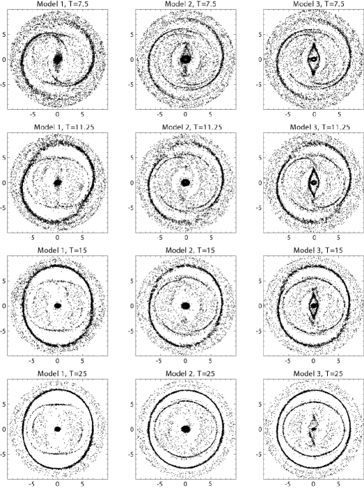
Figure 3: The distribution of OB-particles in models 1–3 at $T=7.5$, $11.25$, $15.0$, and $25.0$.

3 Kinematics of the outer rings and pseudorings

3.1 The resonance kinematics

Table 3: Amplitudes of the velocity oscillations at the distance of $R=7.38$ kpc

Model	1	2	3
T=7.5
$f_{R}$, $f_{\theta}$, km s-1	24, 16	22, 12	24, 13
T=15
$f_{R}$, $f_{\theta}$, km s-1	31, 15	23, 12	25, 12
T=25
$f_{R}$, $f_{\theta}$, km s-1	25, 12	12, 6	15, 8

The modelling suggests that the kinematics of the outer rings and pseudorings is determined by two processes: the resonance tuning and the gas outflow. The resonance kinematics is clearly observed in the pure rings, while the kinematics of the gas outflow is manifested itself in the pseudorings.

Fig. 4 exhibits the distribution of gas particles and OB-particles with the positive and negative residual velocities in projection onto the radial and azimuthal directions at the time moment $T=15$ ($\sim 8$ bar rotation periods). Model 1 was chosen for illustration only, other models display a very similar velocity distribution. The residual velocities were calculated as differences between the model velocities and the velocities due to the rotation curve. The alternation of the quadrants with the negative and positive residual velocities is clearly observed in the pure rings. Besides, particles located at the same azimuthal angle $\theta$ but forming either the $R_{2}$ or the $R_{1}$ ring have the opposite residual velocities. The oscillations of the azimuthal velocities, $V_{\theta}$, are shifted by the angle $\theta\approx\pi/4$ with respect to the radial-velocity oscillations.

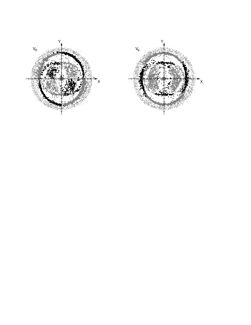
Figure 4: The distribution of particles (gas+OB) with the negative and positive residual velocities in model 1 at the moment $T=15$. The bar is oriented along the Y-axis, the galaxy rotates clockwise, a division on the $X$- and $Y$-axis corresponds to 1 kpc. The left panel represents the radial velocities, while the right one – the azimuthal ones. Only 20% of particles are shown. Particles with the positive residual velocities ($V_{R}>5$ km s^-1 or $V_{\theta}>5$ km s^-1) are indicated by black circles, while particles with the negative ones ($V_{R}<-5$ km s^-1 or $V_{\theta}<-5$ km s^-1) – by grey circles. Particles with the velocities close to zero ($-5<V_{R}<+5$ km s^-1 or $-5<V_{\theta}<+5$ km s^-1) are shown by points.

To study oscillations of the residual velocities we selected particles (gas+OB) located in the narrow annulus of $R=7.38\pm 0.16$ kpc in different models at different moments. Fig. 5 shows the velocity oscillations of selected particles in model 2 at $T=15$. The position of the selected particles corresponds to the average radius of the $R_{2}$ ring. The velocity profiles made at the same radius but for different models and moments resemble each other, the main difference is seen in velocity amplitudes. Table 3 represents the amplitudes of velocity oscillations, $f_{R}$ and $f_{\theta}$, calculated for selected particles in different models at different moments. The highest velocity amplitudes are observed in model 1, while the amplitudes in models 2 and 3 are lower. In each model the lowest velocity amplitudes are observed at $T=25$.

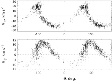
Figure 5: The oscillations of the velocities, $V_{R}$ and $V_{\theta}$, of particles (gas+OB) located in the narrow annulus $R=7.38\pm 0.16$ kpc in model 2 at $T=15$.

We combined the samples of gas particles and OB-particles, because their kinematics is very similar. That is not surprising, because ”OB-associations” in our models have the velocities of their parent gas clouds.

3.2 The orbital kinematics in the resonance region

The resonance between the epicyclic and orbital motions adjusts the epicyclic motions of gas clouds in accordance with orbital rotation. That creates systematical non-circular motions of gas clouds whose direction depends on the position angle of a point with respect to the bar major axis and on the class of the outer ring.

Fig. 6 shows the directions of the residual velocities at the different points of the outer pseudorings. It schematically represents the bar and two main families of periodic orbits. The galaxy rotates clockwise. Motions are considered in the reference frame rotating with the angular speed of the bar. In this frame stars located near the OLR rotate with the speed $(\Omega-\Omega_{b})$ counterclockwise.

Let us consider the family of periodic orbits elongated along the bar and located outside the OLR (Fig. 6). It is represented by the orbit passing through the points 1-2-3-..-8. This family is the backbone of the $R_{2}$ ring. The points 1 and 5 are the peri-centers of the orbit, but the points 3 and 7 are the apo-centers. The epicycles drawing along the border of the figure demonstrate the position of a particle on the epicyclic orbit at the points 1–8. The arrows show the additional velocities caused by the epicyclic motion which can be regarded as the residual velocities. Let us consider the projection of the residual velocities onto the radial and azimuthal directions. At the points 2 and 6 the velocity $V_{R}$ is directed away from the galactic center and achieves its extremal positive value, while at the points 4 and 8 it is directed toward the galactic center and exhibits its extremal negative value. Stars have the negative radial velocities on the orbital segments 3-5 and 7-1 which are marked by dashed lines. Azimuthal residual velocity, $V_{\theta}$, equals zero at the points 2, 4, 6, and 8; it achieves its extremal positive amount at the points 1 and 5 and its extremal negative value at the points 3 and 7.

Another family of periodic orbits oriented perpendicular to the bar is represented by the orbit passing through the points A-B-C-..-H (Fig. 6). The ”dimples” near the points C and G appear due to a relatively large size of the epicycle in comparison with the orbital radius. This family is the backbone of the $R_{1}$ ring. The radial velocity, $V_{R}$, achieves its extremal positive value at the points D and H and the extremal negative one at the points B and F. Points B, D, F, and H are located not at the middles of the corresponding segments but a bit closer to the bar’s ends. The azimuthal velocity, $V_{\theta}$, is zero at the points B, D, F, and H; it achieves its extremal positive value at the points C and G and the extremal negative one at the points A and E.

The directions of the residual velocities in models 1–3 at the moment $T=15$ (Fig. 4) are in a good agreement with the resonance kinematics shown in Fig. 6. Probably, the kinematics of the pure rings (T=15, T=25) is determined by the resonant orbits only.

In the epicyclic approximation the elongation of the outer rings can be explained through the subtraction and addition of the size of the epicycle to the average radius of the ring. In this case the outer rings must demonstrate the following tendency: the smaller the elongation of the ring, the smaller the residual velocities. Models 1–3 confirm this dependence. The outer rings become more round by the time $T=25$ (Fig. 3), that is accompanied with the decreasing velocity amplitudes (Table 3).

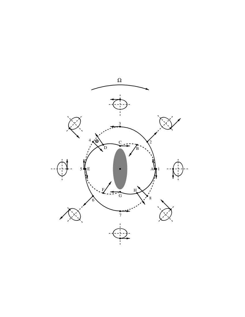
Figure 6: Orbital kinematics in the resonance region. It shows the bar and two main families of periodic orbits in the region of the OLR. The galaxy rotates clockwise. Motions are considered in the reference frame rotating with the speed of the bar. The orbit going through the points 1-2-3-4-5-6-7-8 represents the family of periodic orbits elongated along the bar. The orbit A-B-C-D-E-F-G-H denotes the family of periodic orbits elongated perpendicular to the bar. The epicycles drawing on the border of the picture show the position of a particle on the epicyclic orbit at the points 1–8. The vectors show the directions of the additional (residual) velocities due to the epicyclic motion. The dashed lines indicate the orbital segments with the negative radial velocities, while the solid lines – those with the positive velocities $V_{R}$. The likely position of the Sun is shown by the specific symbol.

3.3 Kinematics of the gas outflow

The main kinematical feature of the outer pseudorings is the preponderance of positive radial velocities against negative ones. All models considered demonstrate the gas outflow at early moments of their evolution. Fig. 7 represents the distribution of particles (gas+OB) with the positive and negative residual velocities in model 1 at $T=7.5$ ($\sim 4$ bar rotation periods), other models have a very similar velocity distribution. Left panel of Fig. 7 clearly shows that particles with the positive radial velocities concentrate to the spiral arms. Right panel of Fig. 7 demonstrates another kinematical feature of the pseudorings: particles located in the inner parts of the spiral arms ($R<R_{OLR}$) have only positive azimuthal velocities $V_{\theta}$, while those forming the outer parts of the spiral arms ($R>R_{OLR}$) have only negative ones.

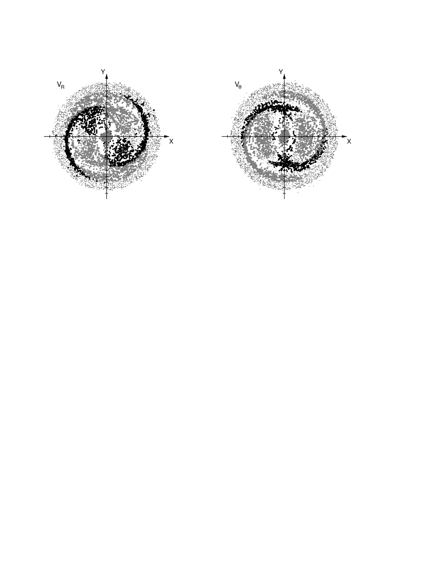
Figure 7: The distribution of gas+OB particles with the negative and positive residual velocities in model 1 at T=7.5. Particles with the positive residual velocities are indicated by black circles, while particles with the negative ones – by grey circles. Particles with the residual velocities close to zero are shown by points. For more details see the caption to Fig. 4.

Schwarz (1981, 1984) finds that the gas outflow to the periphery plays an important role in the formation of the outer rings. Fig. 8 shows the profiles of the surface density of particles (gas+OB) in models 1–3 at different moments. At the initial moment the surface density is constant in the interval $R=1\textrm{--}10$ kpc in all models. At the moment $T=15$ all density profiles have a well-defined maximum corresponding to the location of the $R_{2}$ ring ($R=7\textrm{--}8$ kpc). It grows faster in model 1 than in models 2 and 3 what indicates the more intense gas outflow in model 1. In all models the maximum corresponding to to the $R_{1}$ ring is lying in the vicinity of the outer 4/1 resonance, while the maximum corresponding to the $R_{2}$ ring is shifted $\sim 0.5$ kpc outside the OLR.

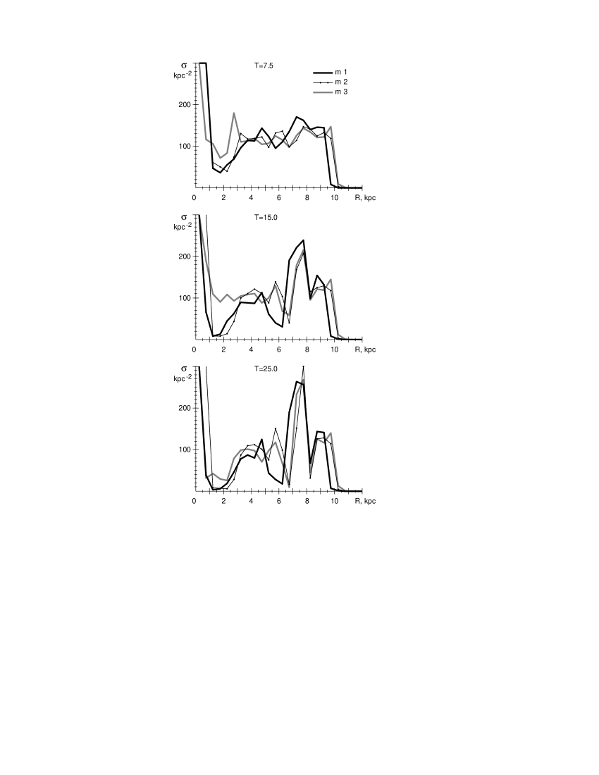
Figure 8: Profiles of the surface density of particles (gas+OB) in models 1–3 at different moments. At the initial moment the surface density is constant in the interval $R=1-10$ kpc.

4 Comparison with the Galaxy

4.1 Positions of the stellar-gas complexes with respect to the outer rings

Let us suppose that the kinematics of young stars in the solar neighborhood is determined by their position with respect to the outer rings. Observations suggest that the Sun goes $\theta_{b}=15\textrm{--}45^{\circ}$ behind the bar elongation, so all complexes studied must be located near the segments 3–5 and C–E of the outer rings (Fig. 6). The Perseus, Cygnus, and Carina regions having the negative velocities $V_{R}$ must belong to the ring/pseudoring $R_{2}$, but the Sagittarius region with the positive velocities $V_{R}$ – to the ring/pseudoring $R_{1}$.

There is some problem with the Perseus ($R=8.4$ kpc) and Carina ($R=6.5$ kpc) regions: they have very different Galactocentric distances $R$ and they both cannot accurately lie on the same ring. Otherwise the ring $R_{2}$ must be highly elongated: the ratio $q$ of the minor and major axis must be of $q\approx 0.6$. However, the observations suggest that the rings/pseudorings $R_{2}$ are not so much elongated: their average axis ratio is $q=0.9$ (Buta and Combes 1996). So the Perseus region must lie a bit outside the $R_{2}$ ring, while the Carina region – a bit inside it.

The kinematics of the Sagittarius region is very important for the definition of a type of the Galactic morphology. The nearly zero residual azimuthal velocities, $V_{\theta}=-1$ km s^-1, here suggest the presence of the $R_{1}$ ring in the Galaxy but not of the spiral arms. Particles located in the inner parts of the spiral arms have only positive velocities $V_{\theta}$ (Fig. 7, right panel) and cannot reproduce $V_{\theta}=-1$ km s^-1. Thus, the Galaxy must also include the $R_{1}$ ring.

4.2 Comparison between models and observations

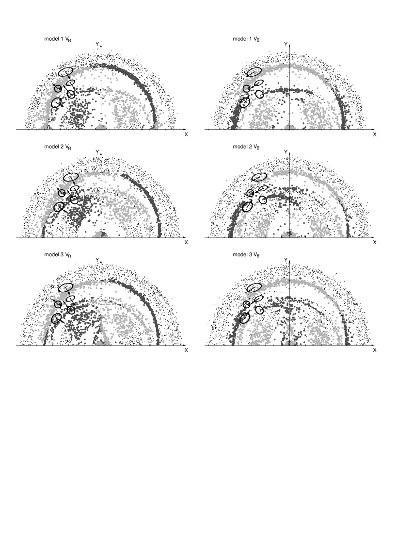
Figure 9: The boundaries of the stellar-gas complexes overlaid above the distribution of particles with the positive and negative residual velocities in models 1–3 at the moment $T=15$. The velocity vectors represent the observed residual velocities. Particles with the positive residual velocities ($V_{R}>5$ km s^-1 or $V_{\theta}>5$ km s^-1) are indicated by black-grey circles, while particles with the negative ones ($V_{R}<-5$ km s^-1 or $V_{\theta}<-5$ km s^-1) – by light-grey circles. Particles with the residual velocities close to zero are shown by points. For more details see the caption to Fig. 4.

Table 4: Model 1. Average residual velocities

Region	$V_{R}$	$\sigma_{R}$	$V_{\theta}$	$\sigma_{\theta}$	n
	km s-1	km s-1	km s-1	km s-1
T=7.5
Sagittarius	21	10	10	12	164
Carina	18	14	8	11	322
Cygnus	-23	3	7	2	33
Local System	-15	4	3	2	63
Perseus	-4	1	-1	2	191
T=15.0
Sagittarius	24	6	0	5	41
Carina	-4	20	10	9	91
Cygnus	-24	4	1	3	18
Local System	-24	3	-5	3	159
Perseus	-4	5	-5	7	207

Table 5: Model 2. Average residual velocities

Region	$V_{R}$	$\sigma_{R}$	$V_{\theta}$	$\sigma_{\theta}$	n
	km s-1	km s-1	km s-1	km s-1
T=7.5
Sagittarius	11	3	0	3	87
Carina	12	4	0	7	183
Cygnus	-16	2	11	2	49
Local System	-13	2	6	4	50
Perseus	-4	2	-2	2	197
T=15.0
Sagittarius	10	3	2	3	98
Carina	9	6	1	8	149
Cygnus	-16	1	8	3	5
Local System	-20	2	1	3	127
Perseus	-7	6	-5	4	187

Table 6: Model 3. Average residual velocities

Region	$V_{R}$	$\sigma_{R}$	$V_{\theta}$	$\sigma_{\theta}$	n
	km s-1	km s-1	km s-1	km s-1
T=7.5
Sagittarius	13	4	-1	4	105
Carina	15	6	1	9	246
Cygnus	-17	2	10	2	31
Local System	-13	2	6	3	43
Perseus	-4	1	-2	1	179
T=15.0
Sagittarius	13	4	1	4	106
Carina	7	9	2	11	138
Cygnus	-18	5	6	2	12
Local System	-21	2	1	3	144
Perseus	-8	7	-6	5	191

Table 7: Comparison between models and observations

Region	$V_{R\mbox{ mod}}$	$V_{R\mbox{ obs}}$	$V_{\theta\mbox{ mod}}$	$V_{\theta\mbox{ obs}}$
	km s-1	km s-1	km s-1	km s-1
Sagittarius	$(+10,+24)$	$+11\pm 3$	$(-1,+2)$	$-1\pm 2$
Carina	$(-4,+9)$	$-6\pm 2$	$(+1,+10)$	$+5\pm 3$
Cygnus	$(-24,-16)$	$-7\pm 3$	$(+1,+8)$	$-11\pm 2$
Local System	$(-24,-20)$	$+5\pm 3$	$(-5,+1)$	$0\pm 3$
Perseus	$(-4,-7)$	$-7\pm 2$	$(-5,-6)$	$-5\pm 2$

To compare models with observations we chose the moment $T=15$ when the resonance kinematics is best-defined. Fig. 9 shows the boundaries of the stellar-gas complexes overlaid above the distribution of particles with the positive and negative residual velocities at the moment $T=15$. The solar position angle is supposed to be $\theta_{b}=45^{\circ}$ in models 1 and 3 and $\theta_{b}=40^{\circ}$ in model 2 (explanation will be given below). Tables 4–6 exhibit the average residual velocities, $V_{R}$ and $V_{\theta}$, of particles located within the boundaries of the stellar-gas complexes in models 1–3 at the moments $T=7.5$ and $15.0$. They also contain the velocity dispersions, $\sigma_{R}$ and $\sigma_{\theta}$, and the number $n$ of particles (gas+OB) which appear to fall within the complex at a certain time moment.

Table 7 represents the model and observed residual velocities for each region. The interval of the model velocities demonstrates the minimal and maximal velocity obtained in models 1–3 at $T=15$.

The Perseus region ($R=8.4$ kpc) has the negative values of the average velocities, $V_{R}$ and $V_{\theta}$, in all models (Table 7). Though the amplitude of the radial velocities at the average distance of the $R_{2}$ ring ($R=7.4$ kpc) is fairly large, $f_{R}=23\textrm{--}31$ km s^-1 (Table 3, $T=15$), its value drops to $f_{R}=4\textrm{--}7$ km s^-1 at the distance of $R=8.4$ kpc. The decrease in the velocity amplitude is due to the fact that the Perseus region is situated a bit outside the $R_{2}$ ring and has less elongated orbit. Altogether, our models reproduce well the kinematics in the Perseus region: the difference between the model and observed velocities don’t exceed 3 km s^-1.

The Sagittarius region ($R=5.6$ kpc) lies near the point D of the $R_{1}$ ring due to the proper scaling and choice of the solar position angle (Fig. 6). Particles located near the point D have the positive velocity $V_{R}$ and nearly zero velocity $V_{\theta}$. Model 1 yields a very large value of the radial velocity, $V_{R}=24$ km s^-1, but models 2 and 3 create the velocities in a reasonable range, $V_{R}=10\textrm{--}13$ km s^-1. In models 2 and 3 the difference between the model and observed velocities don’t exceed 3 km s^-1. Interestingly, that at the moment $T=7.5$ model 1 produces the large positive azimuthal velocity in the Sagittarius region ($V_{\theta}=+10$ km s^-1), but by the moment $T=15$ its value drops to $V_{\theta}=0$ km s^-1 (Table 4). Probably, the large velocity $V_{\theta}$ in model 1 is due to the intense gas outflow at $T=7.5$. Models 2 and 3 do not show such feature (Tables 5-6).

The Carina region ($R=6.5$ kpc) consists of two groups of particles with different velocities (Fig. 9). One group belongs to the ring $R_{1}$, but another – to the ring $R_{2}$. The mixture of two streams produces the larger values of the velocity dispersions, $\sigma_{R}$ and $\sigma_{\theta}$, here in comparison with the other regions (Tables 4-6, $T=15$). The velocities of particles in the ring $R_{2}$ are consistent with observations, so the increase of their relative number in the Carina region brings approaching between the model and observed velocities. All models reproduce the direction of the observed azimuthal residual velocity, but only model 1 reproduces the direction of the radial one. Model 1 has more elongated ring $R_{2}$, what causes more particles of the ring $R_{2}$ to fall within the boundaries of the Carina region. Note that a small rescaling of models can significantly change the average velocity of particles in the Carina region.

The Cygnus region ($R=6.9$ kpc) is located between two outer rings where only a few particles are located. Although the direction of the model radial velocity agrees with observations, its absolute value is too high. As for the azimuthal velocities, none of our models can reproduce the observed negative azimuthal velocity here (Table 7).

The Local System ($R=7.4$ kpc) lies in the vicinity of the $R_{2}$ ring in all models. It contains more particles at the moment $T=15$ than at $T=7.5$. In the context of morphology the moment $T=7.5$ is more suitable for a comparison with observations, because at this moment the break in the $R_{2}$ ring is fairly wide yet (Fig. 3). Our models reproduce well the nearly zero azimuthal velocity, but they cannot create the observed positive radial velocity here (Table 7).

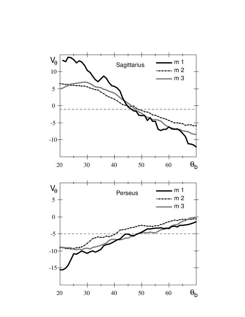
Figure 10: The dependence of the model azimuthal velocity $V_{\theta}$ (km s^-1) in the Sagittarius and Perseus regions ($T=15$, models 1–3) on the solar position angle $\theta_{b}$ (deg.)

Thus, models 2 and 3 reproduce well the values and directions of the residual velocities in the Perseus and Sagittarius regions, but model 1 reproduces the directions of the residual velocities in the Perseus, Sagittarius, and Carina regions. Probably, the kinematics of young stars in the Perseus, Sagittarius, and Carina regions is determined mostly by the resonance, while other processes are dominant in the Cygnus region and in the Local System.

The value of the model azimuthal velocity $V_{\theta}$ in the Sagittarius and Perseus regions is especially sensitive to the choice of the solar position angle $\theta_{b}$. An increase of the angle $\theta_{b}$ causes a decrease of the velocity $V_{\theta}$ in the Sagittarius region and an opposite effect in the Perseus one. Fig. 10 exhibits the variations of the average velocity $V_{\theta}$ in the Sagittarius and Perseus regions with the change of the angle $\theta_{b}$. It is seen that all models reproduce the value of $V_{\theta}=-1$ km s^-1 in the Sagittarius region under $\theta_{b}=45\textrm{--}48^{\circ}$. But in this range model 2 creates the small absolute values of the velocity $V_{\theta}$ in the Perseus region, $|V_{\theta}|=3$ km s^-1. To get the larger value of $|V_{\theta}|$ in Perseus we adopted $\theta_{b}=40^{\circ}$ for model 2.

5 Conclusions

The kinematics of the outer rings and pseudorings is determined by two processes: the resonance tuning and the gas outflow. The resonance kinematics is clearly observed in the pure rings, while the kinematics of the gas outflow is manifested itself in the pseudorings. The resonance between the epicyclic and orbital motion in the reference frame rotating with the bar speed adjusts the epicyclic motions of particles in accordance with the bar rotation. This adjustment creates the systematical non-circular motions, whose direction depends on the position angle of a point with respect to the bar elongation and on the class of the outer ring.

Models of the Galaxy with the $R_{1}R_{2}^{\prime}$ pseudoring reproduce well the radial and azimuthal components of the residual velocities of OB-associations in the Perseus and Sagittarius regions: the difference between the model and observed velocities does not exceed 3 km s^-1 (models 2 and 3, $T=15$). The kinematics in the Perseus region indicates the presence of the $R_{2}$ ring in the Galaxy, while the velocities in the Sagittarius region suggest the existence of the $R_{1}$ ring. The azimuthal velocities in the Sagittarius region accurately defines the solar position angle with respect to the bar elongation, $\theta_{b}=45\pm 5^{\circ}$. Besides, model 1 reproduces the directions of the radial and azimuthal residual velocities in the Perseus, Sagittarius, and Carina regions. Probably, the kinematics of young stars in the Perseus, Sagittarius, and Carina regions is determined mostly by the resonant orbits.

Our models have nearly flat rotation curve. The ring $R_{1}R_{2}^{\prime}$ is forming after several bar rotation periods. The $R_{1}$ ring lies in the vicinity of the outer 4/1-resonance, while the $R_{2}^{\prime}$ pseudoring is shifted $\sim 0.5$ kpc outside the OLR. We found that the mixed $R_{1}R_{2}^{\prime}$ morphology appears when the bar is not very strong: in the case of a strong bar the $R_{1}$ ring disappears. The strong bar and the initial distribution of particles in the disk of a large radius accelerate the formation of the $R_{2}$ rings.

The major semi-axis of the bar in our models has the value of $a=3.8\textrm{--}4.0$ kpc which amounts 55% of the solar Galactocentric distance, $R_{0}=7.1$ kpc, adopted here. The relatively large size of the bar and the large value of the solar position angle, $\theta_{b}=45\pm 5^{\circ}$, agree well with studies in which authors find the presence of a long bar in the Galaxy (Weiner and Sellwood, 1999; Benjamin et al. 2005; Cabrera-Lavers et al. 2007; and other papers).

The model of the Galaxy with the $R_{1}R_{2}^{\prime}$ pseudoring can explain some large-scale morphological features of the Galactic spiral structure. The so-called Carina spiral arm (Russeil 2003) falls nicely onto the segment of the $R_{2}$ ring. Note that two outer rings, which are stretched perpendicular to each other, can look like a 4-armed spiral pattern, especially if the ascending parts of the rings are brighter than the descending ones. But this spiral pattern appears not as a result of the spiral perturbation of the disk potential, but due to the existence of specific orbits in the barred galaxies.