Evolution of Cluster Red-Sequence Galaxies from redshift 0.8 to 0.4: ages, metallicities and morphologies

We present a comprehensive analysis of the stellar population properties (age, metallicity and the alpha-element enhancement [E/Fe]) and morphologies of red-sequence galaxies in 24 clusters and groups from $z\sim 0.75$ to $z\sim 0.45$. The dataset, consisting of 215 spectra drawn from the ESO Distant Cluster Survey, constitutes the largest spectroscopic sample at these redshifts for which such an analysis has been conducted. Analysis reveals that the evolution of the stellar population properties of red-sequence galaxies depend on their mass: while the properties of most massive are well described by passive evolution and high-redshift formation, the less massive galaxies require a more extended star formation history. We show that these scenarios reproduce the index-$\sigma$ relations as well as the galaxy colours. The two main results of this work are (1) the evolution of the line-strength indices for the red-sequence galaxies can be reproduced if 40% of the galaxies with $\sigma<$ 175 kms^-1 entered the red-sequence between $z=0.75$ to $z=0.45$, in agreement with the fraction derived in studies of the luminosity functions, and (2) the percentage the red-sequence galaxies exhibiting early-type morphologies (E and S0) decreases by 20% from $z=0.75$ to $z=0.45$. This can be understood if the red-sequence gets populated at later times with disc galaxies whose star formation has been quenched. We conclude that the processes quenching star formation do not necessarily produce a simultaneous morphological transformation of the galaxies entering the red-sequence.

1 Introduction

Early-type galaxies are strongly clustered (e.g., Loveday et al. 1995; Hermit et al. 1996; Willmer et al. 1998; Shepherd et al. 2001), making galaxy clusters an ideal place for their study. Stellar population studies have shown that both, local and high-redshift early-type galaxies follow tight correlations between the colors and line-strength features and other properties of the galaxies (mostly related with their masses) (e.g. Bower et al. 1992; Kuntschner 2000; Trager et al. 2000a; Bernardi et al. 2005; Sánchez-Blázquez et al. 2006b) The mere existency of these correlations, as well as their evolution with redshift, seem to be consistent with a very early (z$\geq$2) and coordinated formation of their stars (Visvanathan & Sandage 1977; Bower et al. 1992; Ellis et al. 1997; Kodama & Arimoto 1998; Stanford et al. 1998; Kelson et al. 2001; Bender et al. 1998; Ziegler et al. 2001). However, the evolution of the cluster red-sequence luminosity function with redshift challenges this view (De Lucia et al. 2004; De Lucia et al. 2007; Kodama et al. 2004, Rudnick et al. 2008, in preparation; although see Andreon (2008) for contradictory results), and so does the morphological evolution since $z=0.4$ (e.g., Dressler et al. 1997), and the evolution of the blue/star-forming fraction (Butcher & Oemler 1984; Poggianti et al. 2006) in clusters.

A deeper understanding of the nature of the evolution of the cluster red-sequence requires to go beyond colors (affected by the age-metallicity degeneracy) and derive the stellar populations parameters (age and chemical abundances) with time, using stellar population models. However, breaking the age-metallicity degeneracy requires a combination of indices with different sensitivities to both parameters (see, e.g., Rabin 1982). Unfortunately, instrumental limitations have long prevented accurate measurements of absorption line indices at high redshift. Recent observational advances, on the ground and in space, now allow such measurements in intermediate and high redshift galaxies, both in clusters and in the field (Ziegler et al. 2001; Barr et al. 2005; Schiavon et al. 2006; Jørgensen et al. 2005). The analysis of these data have revealed that, indeed, the age-metallicity degeneracy is confusing the interpretation of the scaling relations: large spreads in galaxy luminosity weighted ages and metallicities at high redshift have been found in datasets showing very tight Faber-Jackson, Mgb-$\sigma$ and Fundamental plane (FP) relations, challenging the classical interpretation of the tightness of the scaling relations.

High redshift spectroscopic samples are, however, still restricted to a maximum of $\sim$30 galaxies. Moreover, they often target a single cluster (Kelson et al. 2001; Jørgensen et al. 2005; Tran et al. 2007; Kelson et al. 2006). This could be biasing the results, as studies at low redshift have shown that the star formation histories of early-type galaxies might depend on cluster properties (e.g., compare Kuntschner & Davies 1998; Caldwell et al. 2003; Sánchez-Blázquez et al. 2003; Jørgensen 1999; Nelan et al. 2005; Trager et al. 2008). Therefore, a study based on a large sample of galaxies in clusters covering a large range in cluster masses is necessary to obtain a complete picture of galaxy evolution.

The present work is based on 24 clusters with redshifts between 0.39 and 0.8 from the ESO Distant Cluster Survey (hereafter, EDisCS). The major novelty of the present work is that we do not only consider very massive structures; our sample spans a large range in cluster velocity dispersions. Therefore, we minimize possible biases due to the relationship between galaxy properties and environment.

It is now common to study red-sequence galaxies rather than morphologically classified early-type galaxies, as colours are easier to measure in large datasets than morphology, and they appear to be more correlated with environment (Kauffmann et al. 2004; Blanton et al. 2005; Martínez & Muriel 2006). Nonetheless, observations have also revealed the existence of an intrinsic spread in morphology at given colour (e.g., Conselice 2006; Baldry et al. 2004; Cross et al. 2004). This stress the need for investigating the relation between morphology and colour, and their evolution with redshift and, therefore, this is the strategy we adopt.

Our sample of red-sequence galaxies is much larger than those used in previous efforts. It encompasses 337 galaxies, distributed in 24 clusters and groups, for which we study stellar populations and morphologies. Our sample of red-sequence galaxies is not restricted to the most massive, but span a wide range of internal velocity dipsersion (100-350 km/s), comparable to the samples analysed at low-redshift.

Throughout the paper, we adopt a concordance cosmology with $\Omega_{\rm M}=0.3$, $\Omega_{\Lambda}=0.7$, H₀=70 km s^-1 Mpc^-1. All magnitudes are quoted in the Vega system.

2 The sample

The ESO Distant Cluster Survey (EDisCS) is a photometric and spectroscopic survey of galaxies in 20 fields containing clusters with redshifts between 0.39 and 0.96. These fields were selected from the Las Campanas Distant Cluster Survey (Gonzalez et al. 2001), specifically from the 30 highest surface brightness candidates. A full description of the sample selection can be found in White et al. (2005). EDisCS includes structures with velocity dispersions from $\sim$150 to $\sim$1100 km s^-1, i.e. from small groups to clusters.

Deep optical photometry with VLT/FORS2 (White et al. 2005), near-IR photometry with SOFI on the ESO/NTT (Aragón-Salamanca et al., in preparation), and deep-multi-slit spectroscopy with VLT/FORS2 were acquired for each field. The same high-efficiency grism was used in all observing runs (grism 600RI+19, $\lambda_{0}$ = 6780Å ). The wavelength range varies with the field and the x-location of the slit on the mask (see Milvang-Jensen et al. 2008, for details), but it was chosen to cover, at least, a rest-frame wavelength range from 3670 to 4150 Å (in order to include [OII] and H$\delta$ lines) for the assumed cluster redshift.

The spectral resolution is $\sim$6 Å (FWHM), corresponding to rest-frame 3.3 Å  at $z=0.8$ and 4.3 Å at $z=0.4$. Typically, four- and two-hour exposures were obtained for the high$-z$ and mid$-z$ samples, respectively. The spectroscopic selection, observations, data reduction and catalogs are presented in detail in Halliday et al. (2004) and Milvang-Jensen et al. (2008). In brief, standard reduction procedures (bias subtraction, flat fielding, cosmic-ray removal, geometrical distortion corrections, wavelength calibration, sky subtraction and flux calibration) were performed with IRAF. Particular attention was paid to the sky-subtraction that was performed before any interpolation or rebinning of the data (see Milvang-Jensen et al. 2008, for details). This dataset has also been complemented with 80 orbits of HST/ACS imaging in F814W of the highest redshift clusters (Desai et al. 2007), H$\alpha$ narrow-band imaging (Finn et al. 2005), and XMM-Newton/EPIC X-ray observations (Johnson et al. 2006).

26 structures (groups or clusters) were identified in the 20 EDisCS fields (Halliday et al. 2004; Milvang-Jensen et al. 2008). Two of these structures were not considered in this paper. The first one, cl1103.7-1245, because its spectroscopic redshift (0.96) is too far away from the redshift targeted by the photo-z-based selection (0.70). This can introduce observational biases. The second one, cl1238.5-1144, because it could only be observed for 20 minutes and the S/N of the spectra is not sufficient for our analysis.

To define the red-sequence, we use total-I magnitudes, estimated by adding, to the Kron magnitudes, a correction appropriate for a point source measured within an aperture equal to the galaxy’s Kron aperture. These corrections are obtained empirically from unsaturated and isolated stars on each convolved I-band image (see White et al. 2005 for details).

A galaxy is considered a member of a given cluster (or group) if its redshift falls within 3$\times\sigma_{\rm cluster}$ of the cluster redshift, where $\sigma_{\rm cluster}$ is the cluster velocity dispersion presented in Halliday et al. (2004) and Milvang-Jensen et al. (2008). Similarly to all other EDisCS analyses, galaxy groups are identified by $\sigma_{\rm cluster}<400$ km/s. We define red-sequence galaxies as those with secure redshifts, and colours between $\pm$0.3 mag from the best linear fit (with slope fixed to $-0.09$) to the colour-magnitude relation (V-I vs. I) of the objects without emission lines. This definition coincides with that of White et al. (2005) and De Lucia et al. (2004, 2007). The width of the region corresponds to $\sim$3 times the RMS-dispersion of the red-sequence colours of our two most populated clusters, cl1216.8-1201 and cl1232.5-1250. Table 1 lists the structures selected for the present work and the total number of galaxies on the red-sequence. Figure 1 displays the $V-I$ vs $I$ colour-magnitude diagrams of the 24 EDisCS structures studied in the present paper.

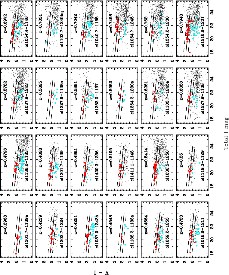
Figure 1: $V$, $I$ colour-magnitude diagrams for the 24 EDisCS structures considered in this study. Galaxies with no- or weak- emission are represented by red circles, while galaxies with strong emission are marked as blue circles. The fit, with a fixed slope of $-0.09$, of the secure cluster members with no or only weak emission is shown as a solid line. The dashed lines trace the $\pm$ 0.3 mag boundary taken into account to select the red-sequence galaxies. This corresponds to the measured dispersions of cl1232.5-1250 and cl1216.8-1201, our two most populous galaxy clusters. When photo-z membership is available, we show the photo-z selected cluster galaxies as small black dots.

To study the evolution of the galaxy population properties with redshift, we divide our galaxies in 3 different redshift intervals : (1) $0.39<z<0.5$; (2) $0.5\leq z<0.65$; and (3) $0.65\leq z<0.81$. For convenience, we refer to these intervals by their median redshifts, $z=0.45$, $z=0.55$, and $z=0.75$. Figure 2 shows the redshift distribution of our sample of galaxies.

Group	Cluster Name	z	ACS	Nreds	NN+W	$\sigma\pm err$	R200
						(kms-1)	Mpc
0.45	cl1018.2-1211	0.4734		17	9	486${}^{+59}_{-63}$	0.93
	cl1037.9-1243a	0.4252	x	18	9	537${}^{+46}_{-48}$	1.06
	cl1059.2-1253	0.4564		26	18	510${}^{+52}_{-56}$	0.99
	cl1138.2-1133	0.4796	x	17	8	732${}^{+72}_{-76}$	1.40
	cl1138.2-1133a	0.4548	x	8	3	542${}^{+63}_{-71}$	1.05
	cl1202.7-1224	0.4240		18	7	518${}^{+92}_{-104}$	1.02
	cl1301.7-1139	0.4828		19	10	687${}^{+81}_{-86}$	1.31
	cl1301.7-1139a	0.3969		13	6	391${}^{+63}_{-69}$	0.78
	cl1420.3-1236	0.4962		18	13	218${}^{+43}_{-50}$	0.41
0.55	cl1037.9-1243	0.5783	x	7	5	319${}^{+53}_{-52}$	0.57
	cl1103.7-1245a	0.6261	x	9	6	336${}^{+36}_{-40}$	0.59
	cl1119.3-1129	0.5500		17	9	166${}^{+27}_{-29}$	0.30
	cl1227.9-1138	0.6357	x	14	8	574${}^{+72}_{-75}$	1.00
	cl1227.9-1138a	0.5826	x	4	1	341${}^{+42}_{-46}$	0.61
	cl1232.5-1250	0.5414	x	41	20	1080${}^{+119}_{-89}$	1.99
	cl1353.0-1137	0.5882		10	7	666${}^{+136}_{-139}$	1.19
	cl1354.2-1230a	0.5952	x	8	5	433${}^{+95}_{-104}$	0.77
	cl1411.1-1148	0.5195		18	12	710${}^{+125}_{-133}$	1.32
0.75	cl1040.7-1155	0.7043	x	14	8	418${}^{+55}_{-46}$	0.70
	cl1054.4-1146	0.6972	x	36	16	589${}^{+78}_{-70}$	1.06
	cl1054.7-1245	0.7498	x	20	6	504${}^{+113}_{-65}$	0.70
	cl1103.7-1245b	0.7031	x	3	2	252${}^{+65}_{-85}$	0.42
	cl1216.8-1201	0.7943	x	38	23	1018${}^{+73}_{-77}$	1.61
	cl1354.2-1230	0.7620	x	7	5	648${}^{+105}_{-110}$	1.05

Table 1: Col. (1) Redshift interval in which the galaxy structure falls (see text for details). Col. (2): Cluster name. Following Milvang-Jensen et al. (2008), we label the secondary structures with letters ”a” and ”b”. Col. (3): Cluster redshift. Col. (4): marked with x if ACS images are available. Col.(5): Number of secure spectroscopically confirmed red-sequence galaxies. Col. (6) Number of red-sequence galaxies with no or negligible emission, full-filling our signal-to-noise ratio criterion. Col. (7) Velocity dispersion of the cluster. Col. (8) R₂₀₀, calculated as in Finn et al. (2005).

Figure 2: Redshift distribution of the red-sequence galaxies in the 3 redshifts-bins with no or negligible emission lines, before any signal-to-noise selection.

Dust reddened star-forming galaxies are estimated to make up $\sim$20% of galaxies in low-redshift clusters (Strateva et al. 2001; Gavazzi et al. 2002; Bell et al. 2004; Franzetti et al. 2007). This contamination is likely to be more important in the strong-emission line regime To avoid contamination from these galaxies that do not have red stellar populations, and due to the difficulty of measuring reliable absorption line indices in galaxies with emission lines, we discard, for our absorption line analysis, galaxies showing evidence of emission lines. Our selection is based both on visual inspection of the 2D- spectra and on measurements of the line equivalent widths (EWs). These measurements were taken from Poggianti et al. (2006). We also measured the [OII] and H$\beta$ emission-line EWs after carefully subtracting the underlying stellar continuum (see Moustakas & Kennicutt 2006 for details). After comparing the visual inspection with the quantitative measurements, we keep galaxies with equivalent widths of [OII]$\lambda$3727 $<7$Å. In Fig. 1 we distinguish between galaxies with strong emission lines and those with no- or weak- emission lines (N+W, hereafter) in the spectroscopic sample of red-sequence galaxies. Figure 3 shows the fraction of N+W red-sequence galaxies as a function of redshift and structure velocity dispersion. The scatter is large and there is no trend with either $\sigma_{\rm cluster}$ or redshift. On average, 24% of the red-sequence galaxies show EW[OII]3727$>$7Å. Section 3 discusses the nature of the emission in these galaxies.

We also remove the brightest cluster galaxies (BCGs) from the sample, as their position in the cluster may lead to a different evolution from the rest of the red population (De Lucia & Blaizot 2007). A photometric study of the BCGs in the EDisCS clusters is presented in Whiley et al. (2008).

Figure 3: Fraction of red-sequence galaxies that have no or only weak emission lines (EW[OII] $<$7$\AA$) as a function of redshift and group/cluster velocity dispersion. This fraction is calculated as the ratio between the N+W red-sequence galaxies and the total number of red-sequence galaxies in the spectroscopic sample.

Our initial sample includes a total of 337 N+W red-sequence galaxies. Their mean spectral signal-to-noise ratio per Å  (S/N), measured between 4000 and 4500 Å  (rest-frame) is $\sim$ 17, 19 and 12 per Å  at redshift 0.45, 0.55 and 0.75, respectively. We consider all galaxies independently of their distance to the cluster centers except for the morphological analysis. The radial cuts, when applied, will be stated explicitly. However, to measure line-strength indices, we require a minimum signal-to-noise ratio of 10 per Å , measured between 4000 and 4500Å  (rest-frame). Thie leave us, for our spectroscopic analysis, with a total of 215 galaxies satisfying our selection criteria, i.e, 70% of the initial sample (see Table 1 for their distribution).

3 Source of ionization for the emission line red-sequence galaxies

As inferred from Fig. 3, a non negligible fraction of red-sequence galaxies exhibit emission lines, with equivalent widths reaching $\sim$30Å  for [OII] and $\sim$12Å  for H$\beta$. Although these galaxies are discarded from further investigation, we are interested in trying to unveil their nature. We investigate below the various possible ionization sources and look for evidence of evolution with redshift.

We perform a similar analysis than Yan et al. (2006). Yan et al. (2006) studied a large sample of red galaxies from the Sloan Digital Sky Survey (SDSS) finding emission in 52.2% of them. They showed that they could be classified in two main groups: galaxies with high [OII]$\lambda 3727\AA$/H$\alpha$ (LINER-like and quiescent galaxies, representing 20.6% of the total red populution with emission) and low-[OII]/H$\alpha$ galaxies (mostly dusty-starforming ones, with a small fraction of Seyferts, accounting for 9% of the red-sequence galaxies with emission). Counting galaxies with only [OII] seen in emission (instead of both [OII] and H$\alpha$) increases the fraction of LINERS to 28.8%. Finally, 14% of the red galaxies have H$\alpha$ detected but no [OII], making them difficult to classify. Nevertheless, Yan et al.  (2006) show that the majority of these galaxies have [NII]/H$\alpha>0.6$ suggesting a non-starforming origin for their emission lines.

In the present case, the determination of the ionization sources is hampered by the fact that the wavelength coverage of the spectra does not include H$\alpha$. We consider H$\beta$ instead. For each galaxy, the stellar continuum has been fitted and the [OII] and H$\beta$ equivalent widths subsequently measured. Figure 4 illustrates the distribution of [OII] and H$\beta$ EWs for the red-sequence galaxies and for the full EDisCS spectroscopic sample.

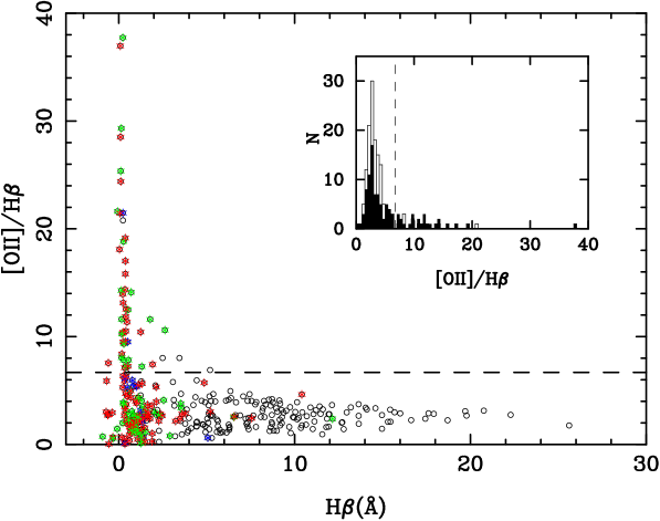
Figure 4: Ratio between [OII] and H$\beta$ for the full EDisCS sample of cluster members (black dots). Red, green, and blue stars indicate the red-sequence galaxies in the 0.45, 0.55, and 0.75 redshift bins, respectively. The[OII]/H$\beta$ distribution is also presented in the form of a histogram: the black-filled zone represents the red-sequence galaxies, to be compared to the full sample. Dashed lines indicate the [OII]/H$\beta$ = 6.7 limit above which the galaxy emission is considered to be due to mechanisms other than star formation.

Out of the EDisCS full sample of red-sequence galaxies (393), 243 have spectra with a wavelength range appropriately centered and wide enough to include both [OII]$\lambda\lambda 3727$Å  and H$\beta$. The redshift distribution of these galaxies has a mean of 0.52 and a standard deviation of 0.09. We count 57 galaxies with a 2-$\sigma$ detection (threshold identical to Yan et al. (2006)) of both [OII] and H$\beta$, 68 with only one of the two lines detected, and 118 with no detection at all (at the 2-$\sigma$ level). Hence, very similarly to Yan et al. (2006), we obtain 51.4% of emission line red-sequence galaxies.

Following Kewley et al. (2004), we consider that star formation cannot induce [OII]/H$\alpha$ larger than 1.5. This value is derived before any reddening correction and was independently confirmed by Moustakas & Kennicutt (2006). We assume a mean value of H$\alpha$/H$\beta$=4.46, which was derived by Yan et al. (2006) before any reddening correction, and which corresponds to a median extinction of A_V=1.40, assuming Type B recombination. Under this condition, [OII]/H$\beta$= 6.7 draws a boundary between star forming galaxies and those with emission powered by an AGN. As shown in figure 11 of Yan et al. (2006), this limit is very conservative. Indeed, one hardly finds any star forming galaxies with [OII]/H$\beta$ $>$ 5. However, it does eliminate most Seyferts and selects mostly LINER-type galaxies. Interestingly, the limit of 6.7 seems to represent a natural upper limit for the bulk of the whole cluster galaxy population (see the histogram part of Figure 4). For our statistics below, we use the empirical bimodal demarcation advised by Yan et al. (2006), i.e., EW([OII])=18EW(H$\beta$)$-$6 rather than a constant [OII]/H$\beta$ ratio. We have checked, however, that both methods lead to identical results (within 1-2%).

Table 2 shows the emission-line properties of the red-sequence galaxies with spectra wide enough to cover H$\beta$ and [OII]. To go beyond upper and lower limits we would need, at least, another set of two lines to build more diagnostic diagrams (e.g., Kewley et al. 2006). However, we believe that our counts give reliable hints on the major trends for the ionization processes at play in our sample. The fraction of quiescent red galaxies is very much the same as the percentage reported by Yan et al. (2006) in the local Universe. The obvious difference between the two studies resides in the nature of the galaxies which do have detections of both H$\beta$ and [OII]. While Yan et al. (2006) find that only 9% of those galaxies have low-[OII]/H$\beta$ ratios, we obtain more than twice this percentage, 19%. In addition, only 4% of our red-sequence galaxies have high-[OII]/H$\beta$ ratios characteristic of LINERS. This fraction might increases up to 8% if we include galaxies with [OII] detected and H$\beta$ undetected. However, this is still a factor of 3 smaller than the fraction of high-[OII]/H$\beta$ galaxies in the red-sequence reported by Yan et al. (2006), 29%.

The conclusion for this tentative identification of the ionizing sources in the EDisCS emission line red-sequence galaxies is that most of them are dusty star forming ones. We can not disentangle, at this stage, whether time or environment, or even more technically the use of H$\beta$ instead of H$\alpha$, leads to the difference with the results of Yan et al. (2006). Further investigation, both in field intermediate redshift galaxies and in low redshift cluster galaxies, is required to shed light on this matter.

[OII]	H$\beta$	[OII]/H$\beta$	Fraction
N	N		48.5 %
N	Y	uncertain	24 %
Y	N	high	4%
Y	Y	high	4%
Y	Y	low	19.5%

Table 2: Emission line properties of the red-sequence galaxies for which the spectra covers both [OII] and H$\beta$. The first two columns indicate whether or not [OII] and H$\beta$ have been detected (at 2-$\sigma$ level). High and low [OII]/H$\beta$ stand for EW([OII])$>$18EW(H$\beta$)$-$6 and EW([OII])$<=$18EW(H$\beta$)$-$6, respectively.

4 Stellar velocity dispersions

Velocity dispersions were measured in all our spectra using the IDL routine PPXF developed by Cappellari & Emsellem (2004). This routine, based on maximum penalized likelihood with optimal template, is specially suited to extract as much information as possible from the spectra while suppressing the noise in the solution and, therefore, is perfect to measure the kinematics in low S/N data. This algorithm estimates the best fit to a galaxy spectrum by combining stellar templates that are convolved with the appropiate mean galaxy velocity and velocity dispersion. The final values of these parameters are sensitive to the template missmatch and, therefore, the use of this technique requires templates which match closely the galaxy spectrum under scrutiny. This is achieved with the use of extensive stellar library spanning a large range of metallicities and ages. We use 35 synthetic spectra from the library of single stellar population models from Vazdekis et al. (2009, in preparation), which makes use of the new stellar library MILES (Sánchez-Blázquez et al. 2006c), degraded to the resolution of EDisCS spectra. The library contains spectra spanning an age range from 0.13 to 17 Gyr and metallicities from $[$Z/H$]=-0.68$ to $[$Z/H$]=+0.2$. Errors were calculated by means of Monte Carlo simulations, in which each point was perturbed with the typical observed error, following a Gaussian distribution. Because the template mistmach affects the measure of the velocity and $\sigma$ determined with PPXF, a new optimal template was derived in each simulation. The errors were obtained as the standard deviation of a total of 50 simulations. The mean uncertainty in the velocity dispersion calculated in our spectra with S/N $>$ 10 is $\sim$25%. Given the signal-to-noise ratio and the resolution of our spectra, $\sigma$ values below 100 kms^-1 are considered untrustworthy and, consequently, galaxies with $\sigma<100$ kms^-1 are eliminated in all analysis involving the comparison with $\sigma$.

5 Line-strength indices

For all of the galaxies in the red sequence, we measure Lick/IDS indices as defined by Trager et al. (1998) and Worthey & Ottaviani (1997). The strength of the Lick/IDS as a function of age, metallicity, and individual chemical abundances has been calibrated by many authors for a simple stellar population, i.e. a population formed in a single, instantaneous burst (e.g. Worthey 1994; Vazdekis 1999; Thomas et al. 2003, TMB03 hereafter), and for more complicated star formation histories (e.g. Bruzual & Charlot 2003). These indices remain the most popular way to extract information about the stellar ages and metallicities from the integrated light of galaxies.

The errors on the indices were estimated from the uncertainties caused by photon noise using the formula by Cardiel et al. (1998) and from uncertainties due to the wavelength calibration, derived using Monte-Carlo simulations. The variances were estimated from the residuals between the observed spectrum and the $"$best template$"$, which was obtained in the calculation of the velocity dispersion, and which was previously broadened to match the line width of each galaxy. For the clusters with $z>0.6$, indices redward of 4500 Å  were affected by telluric absorption in the atmosphere and by sky subtraction residuals and were not measured. For the clusters with $z\sim 0.45$ all Lick/IDS indices from H$\delta_{A}$ to H$\beta$ were measured, as well as D4000. Each individual spectrum was visually examined to check for indices affected by sky residuals or telluric absorption in the atmosphere. All affected indices were discarded from any subsequent analysis.

Line-strength indices are sensitive to the line broadening due to both instrumental resolution and the stellar velocity dispersion. In order to compare the galaxy spectra with stellar population models and to compare the line-strength indices of galaxies with different velocity dispersion, the indices need to be corrected to identical levels of intrinsic Doppler and instrumental broadening.

Because the models we are using (see Sec. 6) predict, not only line-strength indices, but the whole spectral distribution, we can degrade the synthetic spectra to the resolution of the data. We decided to broaden all of the observed and synthetic spectra to a final resolution of 325 km s^-1 (including the velocity dispersion of the galaxy and the instrumental resolution) before measuring the indices. Galaxies with a velocity dispersion higher than $\sim$ 315 km s^-1 could not be broadened, but the number of galaxies with velocity dispersions above this limit is very small and, therefore, we decided to include them on the plots, although they have not been included in the data analysis.

One of the problems of using Lick/IDS-based models (e.g., Worthey 1994; Thomas, Maraston & Bender 2003) is that the data need to be transformed to the spectrophotometric system of the Lick/IDS stellar library. To do this, it is common to observe stars from the Lick/IDS library using the same instrumental configuration than for the science objects and to derive small offsets between the indices measured in those stars and the ones from Lick/IDS. When analyzing data at high redshift, this is of course impossible. In principle, no further corrections to the indices are required when comparing data with stellar population models using flux-calibrated libraries. Although we do not have to apply the offsets to our indices, we have computed them using the stars in common between MILES and the Lick/IDS library because it may be useful for other studies. The final offsets and the comparison can be found in Appendix A .

Some of the Lick/IDS indices are affected by emission lines. In particular, emission, when present, fills the Balmer lines, lowering the values of the indices and, hence, increasing the derived age. High-order Balmer indices (H$\delta$ and H$\gamma$) are much less affected by emission than the classic index H$\beta$ (Worthey & Ottaviani 1997), but nevertheless still affected. To correct for emission, two different approaches are normally adopted: First, assume a correlation between the equivalent width of some other emission line and the emission in the Balmer line (e.g. Trager et al. 2000a). Second, fit an optimal template and subtract the emission directly from the residuals. Nelan et al. (2005) have shown that the first approach suffers from significant uncertainties, in part because there are almost certainly several competing sources of ionization in early type galaxies. The second approach requires that the fit of the optimal template to the individual spectrum is very good. The S/N of our individual spectra simply do not allow us to explore that option. Therefore, instead of trying an emission correction to the Balmer lines, we have analyzed the differences in the results by first eliminating all the galaxies showing any emission. It is re-assuring to see that none of our conclusions change when the (weak) emission line galaxies are excluded (we remind the reader than the galaxies with strong emission lines have been excluded from the analysis).

Table 3, available at the CDS, lists the measured line-strength indices in our sample of galaxies with non-or weak emission lines. A portion of the table is shown here to show its content an structure.

Table 3: Line-strength indices in our sample of red-galaxies with S/N(Å)$>$10 and no- or weak-emission lines. The number between brackets after the indices values indicates the presence (1) or not (0) of sky-subtraction residuals or telluric absorptions inside the definition passband of the index. Only those indices with labels (0) are used in our analysis. Type: Indicate the presence (2) or not (1) of weak ([OII]$<$7Å) emission lines. Last column lists the measured velocity dispersion and its error. This is only a portion of the Table, shown for guidance regarding its format and content. The full table is electronically available at CDS and at http://www.ucm.es/info/Astrof/psb/ediscs.html.

	D4000	H$\delta_{A}$	H$\delta_{F}$	CN2	Ca4227	G4300	H$\gamma_{A}$
1018471-1210513	1.83$\pm$0.01 (1)	1.28$\pm$0.41 (0)	2.11$\pm$0.27 (0)	0.027$\pm$0.015 (0)	1.27$\pm$0.23 (0)	2.71$\pm$0.43 (0)	$-1.53\pm$0.47 (0)
1018464-1211205	2.22$\pm$0.02 (1)	$-0.18\pm$0.69 (0)	0.84$\pm$0.47 (0)	0.038$\pm$0.024 (0)	0.87$\pm$0.38 (0)	4.86$\pm$0.65 (0)	$-4.75\pm$0.81 (0)
1018467-1211527	2.13$\pm$0.01 (0)	$-0.97\pm$0.29 (0)	0.63$\pm$0.19 (0)	0.108$\pm$0.010 (0)	0.48$\pm$0.16 (0)	5.10$\pm$0.26 (0)	$-5.55\pm$0.33 (0)
1018401-1214013	1.98$\pm$0.02 (0)	$-0.57\pm$0.65 (0)	0.40$\pm$0.45 (0)	0.072$\pm$0.022 (0)	0.53$\pm$0.37 (0)	7.13$\pm$0.57 (0)	$-4.71\pm$0.76 (0)
	H$\gamma_{F}$	Fe4383	Ca4455	Fe4531	type	$\sigma\pm$err
1018471-1210513	0.52$\pm$0.28 (0)	3.71$\pm$0.68 (0)	0.67$\pm$0.38 (0)	3.28$\pm$0.58 (0)	2	245.9$\pm$15.8
1018464-1211205	$-2.01\pm$0.52 (0)	4.10$\pm$1.09 (0)	0.91$\pm$0.60 (0)	3.47$\pm$0.93 (0)	1	279.9$\pm$27.6
1018467-1211527	$-1.73\pm$0.21 (0)	3.27$\pm$0.44 (0)	0.98$\pm$0.24 (0)	3.03$\pm$0.38 (0)	1	211.1$\pm$14.8
1018401-1214013	$-0.29\pm$0.45 (0)	1.77$\pm$1.06 (0)	0.71$\pm$0.57 (0)	1.37$\pm$0.91 (0)	1	129.2$\pm$21.0

5.1 The local sample & aperture correction

To increase the time baseline of our analysis, we compare the EDisCS spectra with 36 early-type galaxies (ellipticals and lenticulars) in the Coma cluster at redshift $z=0.02$. The characteristics of this sample are described in Sánchez-Blázquez et al. (2006b). Because the galaxies were selected morphologically we checked first that all the objects belong to the red-sequence of this cluster, using the colours and magnitudes from Mobasher et al. (2001). We are aware that the comparison with the Coma cluster is probably not the most appropriate, as the the velocity dispersion of this cluster exceeds that of all the clusters in our sample at intermediate redshifts. For this reason, we will base all the conclusions of this paper in the intercomparison of the EDisCS clusters. The local sample is included here to show that some of our results can be extrapolated to the local Universe, where higher S/N spectra can be obtained. One of the main problems when comparing observations at different redshifts is that, for a fixed aperture, one is sampling different physical regions within the galaxies. Early-type galaxies show variations in their main spectral characteristics with radius and, therefore, a correction due to these aperture differences is necessary. In order to compare directly with the sample at medium- and high-redshift, we extracted the 1D spectra in the same way as the EDisCS spectra, inside an aperture equal to the FWHM of the spatial profile. However, aperture effects are not entirely mitigated via such an extraction, as the EDisCS spectra were observed with a 1^′′-wide slit, equivalent to a much larger physical aperture at the redshift of the Coma cluster. Jørgensen et al. (1995), Jørgensen (1997) and Jørgensen et al. (2005) derived aperture corrections using mean gradients obtained in the literature. The index corrected for aperture effects can be obtained as $\log(\rm index)_{\rm corr}=\log(\rm index)_{\rm ap}+\alpha\log\frac{\rm r_{\rm ap}}{\rm r_{\rm nor}}$ for those indices measured in Å  and ${\rm index}_{\rm corr}={\rm index}_{\rm ap}+\alpha\log\frac{\rm r_{\rm ap}}{\rm r_{\rm nor}}$ for molecular indices measured in magnitudes, where ${\rm r_{\rm nor}}$ is the final normalised aperture, and $r_{\rm ap}$ is the equivalent circular aperture, obtained as 2 ${\rm r}_{\rm ap}=1.025\times 2(xy/\pi)^{1/2}$, being ${x}$ and ${y}$ the width and length of the rectangular aperture. Jørgensen (1995, 1997) calculated $\alpha$ parameters for a large subset of Lick indices but, in some cases, using the gradients measured in a very small sample of galaxies. In this work, we have taken advantage of the large sample of galaxies with measured line-strength gradients published in Sánchez-Blázquez et al. (2006a), Sánchez-Blázquez et al. (2007) and Jablonka et al. (2007) to calculate new aperture corrections. These also include corrections for the higher-order Balmer lines that have not been published before, as far as we are aware. Appendix B lists the new $\alpha$ parameter calculated in this paper. We correct all our indices to mimic the physical aperture of the slit used to observe the galaxies at $z=0.75$. The aperture corrections ($\alpha\log\frac{\rm r_{\rm ap}}{\rm r_{\rm nor}}$) for all the indices at the different redshift bins are listed in Table 4.

Index	Coma	$z=0.45$	$z=0.55$	$z=0.75$	correction type
H$\delta_{A}$	1.031	0.063	0.016	0.00	additive
CN1	$-0.083$	$-0.005$	$-0.001$	$0.00$	additive
Ca4227	0.856	0.990	0.997	1.0	multiplicative
G4300	0.914	0.995	0.998	1.0	multiplicative
H$\gamma_{F}$	0.623	0.038	0.009	0.0	additiva
Fe4383	0.817	0.987	0.996	1.0	multiplicative
Ca4455	0.726	0.980	0.995	1.0	multiplicative
Fe4531	0.876	0.992	0.998	1.0	multiplicative
C4668	0.676	0.976	0.994	1.0	multiplicative
H$\beta$	1.179	1.010	1.000	1.0	multiplicative

Table 4: Aperture correction for Lick/IDS indices measured in our sample. The correction for the molecular indices and for the higher-order Balmer lines is additive while the correction for the atomic indices is multiplicative. The aperture correction was only applied to the Coma galaxies, as it is very small for the other redshifts. The type of correction is indicated in the last column.

Line-strength gradients show large variations between early-type galaxies (see, e.g. Carollo et al. 1993; Gorgas et al. 1990; Davies et al. 1993; Halliday 1998; Sánchez-Blázquez et al. 2006a; Kuntschner et al. 2006; Jablonka et al. 2007, among others), and the slope of the gradients does not seem to correlate clearly with any of their other properties. For this reason, we use the mean gradient to compute the aperture corrections for all the galaxies. However, in order to calculate the error in the aperture correction due to the fact that early-type galaxies show a large variation in the slope of their gradients, we perform a series of Monte Carlo simulations where the mean index-gradient was perturbed by a random amount, given by a Gaussian distribution with $\sigma$ equal to the typical RMS- dispersion in the gradients The errors in the aperture correction calculated this way are also indicated in Table 4. In some cases (e.g., higher-order Balmer lines), these errors are very large. In fact, despite the large mean aperture correction for H$\delta$ and H$\gamma$ indices, the aperture correction is compatible, within those errors, with being null. These errors have been added quadratically to the errors of the indices for the Coma galaxies. For the 0.45 and 0.55 bins, the error in the aperture correction due to the scatter among the mean gradients is negligible (less than 1% of the total correction) and we do not list them.

Gradients might evolve with redshift. That is the reason why we correct the indices in the Coma cluster to the same equivalent aperture as the highest redshift bin instead of correcting the highest redshift measurements as is commonly done. This way, the correction is performed to the galaxies where the gradients used to derive the aperture correction have been measured.

5.2 Stacked spectra

The degeneracy between age and metallicity effects on galaxy colours could well affect the interpretation of their colour-magnitude diagrams. This degeneracy can be partially broken by using a combination of two or more spectral indices chosen for their different sensitivities to age and metallicity. The S/N of our galaxy spectra is not high enough to do this analysis on an individual basis. Therefore, in order to derive the evolution with time of the galaxy mean ages and chemical abundances, we stacked the galaxy spectra in each of the 0.45, 0.55 and 0.75 redshift bins.

We made sure that the distribution of galaxy velocity dispersions ($\sigma$) in all the different redshift intervals is similar (Fig. 5). This a prerequisite to any further comparison between the three redshift bins, as most line-strength indices are strongly correlated with this parameter (e.g. González 1993). To explore the possible dependence of star formation history on galaxy mass, we distinguish between galaxies with $\sigma$ higher and lower than 175km s^-1 in all three redshift groups. We perform a Kolmorogov-Smirnov test comparing the distribution of $\sigma_{\rm s}$ at different redshifts to look for possible significant differences. We performed the test separately for galaxies with $\sigma$ larger and smaller than 175 km s^-1 and found them compatible with being drawn from the same distribution.

Before adding them, we normalize all spectra by their mean flux in the region between 3900Å  and 4400Å, to avoid a bias towards the indices of the most luminous galaxies. Finally, we co-add them, clipping out all the pixels deviating more than 2-$\sigma$ from the mean. Figure 6 displays the resulting 6 stacked spectra for the three redshift bins and the two velocity dispersion regimes.

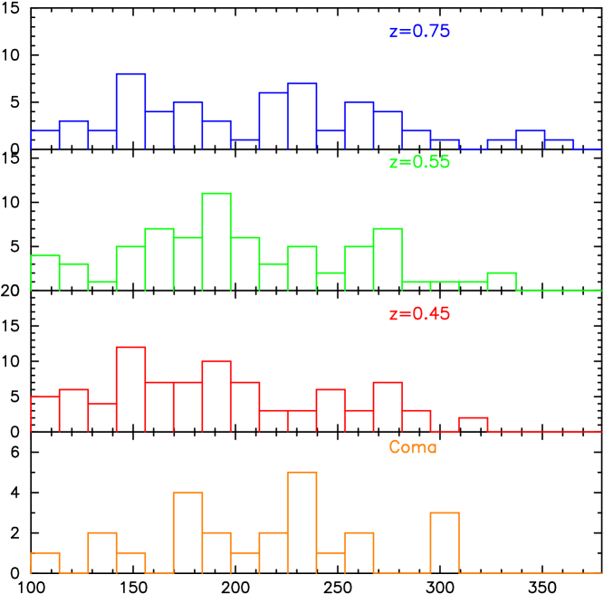
Figure 5: Velocity dispersion distribution of the individual spectra stacked in the different redshift bins. From bottom to top: $z$=0,0.45,0.55,0.75.

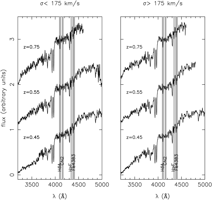
Figure 6: Final stacked spectra for our three redshift and velocity dispersion bins. The shaded areas identify the central bands of the four indices used in our spectral analysis.

Earlier works have studied the evolution of red-sequence galaxies as a function of magnitude (e.g. De Lucia et al. 2004; De Lucia et al. 2007; Rudnick et al. 2008, in preparation). These studies have put the boundary between faint and bright galaxies at Mv$=-20$. Assuming a formation redshift of 3 followed by passive evolution, our $\sigma$=175 km s^-1 cut corresponds to Mv$\sim-$20.0, $-20.2$ and $-20.2$ mag at $z=0.45$, 0.55 and 0.75, respectively (see Figure 7). As can be seen, the magnitude cut is not very different between our study and the above mentioned photometric studies. However, those studies reach much fainter magnitudes in their $"$faint$"$ bin.

Figure 7: Relation between the absolute magnitude Mv and the velocity dispersion for our sample of galaxies in the three considered redshift bins. The right label shows the absolute magnitude Mv evolved passively to $z=0$ using Bruzual & Charlot (2003) models at solar metallicity. The vertical dashed line indicates the position corresponding to our $\sigma$-cut (175 km s^-1) while the horizontal line marks the mean magnitude for the galaxies with a sigma between 160 and 180 km ^-1.

Velocity dispersions and line-strength indices for the stacked spectra were measured using the same techniques as for the individual spectra. Errors on the indices were calculated with the formula of Cardiel et al. (1998), using the signal-to-noise of the stacked spectra. These errors do not reflect the differences between the spectra added in each bin, which are larger than the formal errors obtained using the signal-to-noise ratio. However we do not intend to study the distribution of galaxy properties but rather their mean values. To explore the robustness of our results to errors in velocity dispersion, we performed 20 Monte Carlo simulations in which the individual galaxy velocities were randomly perturbed following a Gaussian error distribution. After each simulation, the spectra were stacked again, indices were measured, and their mean and RMS-dispersion were calculated. Fig. 8 compares the indices obtained in the original stacked spectra with the mean indices obtained from the 20 simulations. The separation in low- and high-$\sigma$ galaxies is robust to the errors in velocity dispersion. When the RMS-dispersion for all the simulated galaxies is larger than the error we have calculated for the individual indices, we add the quadratic difference as a residual error to the original error in the index. We have also checked that the mean values of the individual indices for all the stacked galaxies is compatible, within the errors, with the index measured in the stacked spectra.

The Lick/IDS indices measured in the stacked spectra as well as their errors are listed in Table 5.

Redshift group		D4000	H$\delta_{A}$	H$\delta_{F}$	CN2	Ca4227	G4300	H$\gamma_{A}$	H$\gamma_{F}$	Fe4383	$\sigma$
		Å	Å	Å	mag	Å	Å	Å	Å	Å	kms-1
0.45	$\sigma>175$ km/s	2.044	$-0.433$	0.894	0.067	0.932	4.589	$-4.114$	$-0.704$	3.662	233.1
		0.004	0.140	0.094	0.005	0.076	0.133	0.161	0.098	0.220	7.2
0.45	$\sigma<175$ km/s	2.045	0.103	1.074	0.036	0.841	4.053	$-3.145$	$-0.177$	3.380	122.3
		0.004	0.139	0.094	0.005	0.077	0.136	0.158	0.096	0.222	12.0
0.55	$\sigma>175$ km/s	2.051	$-0.075$	1.143	0.065	0.847	4.600	$-3.779$	$-0.437$	3.534	218.1
		0.002	0.087	0.058	0.003	0.048	0.083	0.100	0.061	0.137	9.0
0.55	$\sigma<175$ km/s	1.995	0.045	0.960	0.028	0.757	4.341	$-3.138$	$-0.114$	3.138	134.9
		0.004	0.140	0.095	0.005	0.078	0.135	0.159	0.096	0.224	10.1
0.75	$\sigma>175$ km/s	2.008	0.699	1.400	0.057	0.824	4.381	$-3.061$	$-0.234$	2.877	233.2
		0.003	0.104	0.070	0.004	0.059	0.102	0.120	0.073	0.171	6.2
0.75	$\sigma<175$ km/s	1.987	0.453	1.163	0.034	0.826	4.244	$-2.963$	$-0.016$	2.796	154.2
		0.003	0.130	0.089	0.004	0.073	0.128	0.149	0.091	0.213	8.1

Table 5: Line-strength indices and velocity dispersion measured in the stacked spectra. The second row of each line lists the errors. Last column show the velocity dispersion measured in the different stacked spectra.

Figure 8: Comparison between the indices measured in the stacked spectra and the mean index calculated in the 20 stacked spectra obtained with Monte Carlo simulations as described in the text to analyze the robustness of our separation of galaxies with $\sigma$ due to errors in this parameter. The errors in the $y$-direction represent the rms of all the 20 measured indices, while the errors in the $x$-direction represent the errors in the index due to the S/N of the stacked spectra. Big and small symbols show the indices measured in the stack with $\sigma$ larger than 175 kms^-1 and smaller than $\sigma<175$ kms^-1 respectively. The meaning of the different symbols is indicated in the inset.

6 Stellar population models

In this study we compare our measured values with the models by Vazdekis et al.  (2008, in preparation, V08 hereafter). These models are based on the MILES stellar library (Sánchez-Blázquez et al. 2006c). The spectra from this library have a resolution of 2.3Å , constant along the whole wavelength range, and are flux-calibrated. Thanks to this, the models predict not only individual indices, but the whole spectral energy distribution from 3500 to 7500Å  as a function of age and metallicity, for ages between 0.1 and 17.78 Gyr and metallicities from [Z/H]=$-1.68$ to +0.2 dex.

However, the chemical composition of stars in the MILES library (as in the rest of empirical libraries included in stellar population models) matches that of the solar-neighborhood. This means that the models, in principle, can only predict accurate ages and metallicities for stellar populations with the same chemical patterns as the solar vicinity. We know that this condition does not apply to bright nearby early-type galaxies (see review by Worthey 1998)), where Mg/Fe and maybe Ti/Fe, Na/Fe, N/Fe and C/Fe are enhanced with respect to the solar values. This may result in systematics errors in the measured ages and metallicities (see Worthey 1998; Thomas et al. 2003). In order to overcome this problem, we calibrate the models for different chemical compositions using the method first introduced by Tantalo et al. (1998) and Trager et al. (2000a). This method uses stellar atmospheres to characterize the variation of the different indices to relative changes of different chemical species. We first interpolate the existing models to make a grid with 168 ages from 1 Gyr to 17.8 Gyr in steps of 0.1 Gyr and 209 metallicities from $-1.68$ to +0.4 in steps of 0.1. Then, we modify each index according to their fractional response to variations of different elements using (from Trager et al.):

$$\frac{\Delta I}{I}=\left(\prod_{i}(1+R_{0.3}(X_{i}))^{[X_{i}/H]/0.3}\right)-1,$$ (1)

where $R_{0.3}(X_{i})$ is the response function for element $i$ at $[X_{i}/H]=+0.3$ dex. As in Trager et al. , we also consider that the fractional light contribution from each stellar component is 53% from cool giant stars, 44% from turnoff stars and 4% from cool dwarfs stars. We use the calibrations by Korn et al. (2005) instead of the ones by Tripicco & Bell (1995) (used by Trager et al.) because they include the higher order Balmer lines H$\delta$ and H$\gamma$, and they are computed at other metallicities different from solar. However, the differences between the two studies are very small (Korn et al. 2005). Following the approach of several previous authors, we do not change all the elements individually but we assume than some of them are linked by nucleosynthesis and, therefore, change them in lock-step. We built models where N, Ne, Na, Mg, Si and S are enhanced by 0.3 dex with respect to Fe while C is enhanced by +0.15 dex. The reason that C is only enhanced by +0.15 is that enhancing C by +0.3 dex brings the C/O ratio very close to the values at which a carbon star is formed (see Houdashelt et al. 2002; Korn et al. 2005, for a discussion). Ca and the Fe peak elements are depressed to keep the overall metallicity constant. To obtain response functions for enhancements different from +0.3 dex we, again, follow Trager et al. (2000b): We first calculate $\Delta$[Fe/H] and $\Delta$[E/Fe] using $\Delta$[Fe/H]=$-$A$\Delta$[E/Fe] = $-\frac{A}{1-A}\Delta$[E/H], where E represents the enhanced elements. $A$ is the response of the enhanced elements to changes in [Fe/H] at fixed [Z/H]. For the chosen enhanced model, $A=0.929$ (Trager et al. 2000). Then, we scale exponentially the response functions by the appropriate element abundance. We built models with enhancements from [E/Fe]=$-0.1$ to $0.5$ in steps of 0.05.

Because we are not working at the Lick/IDS resolution, in principle, we should not be using Korn et al. (2005) response functions to compute the sensitivity of different indices to variations of chemical abundance ratios, as they were computed at this resolution. However, Korn et al. (2005) showed that the influence of the resolution on the response functions is very small.

Note that the models used here (as well as most existing models in the literature) do not include isochrones with chemical abundance ratios different from solar. The effect of the different chemical abundance ratios is only included in the atmospheres. The influence that the inclusion of $\alpha$-enhanced isochrones may have in the final predictions is still unclear, especially at super-solar metallicities, but some studies have shown that it is much smaller than the one in the model atmospheres (Coelho et al. 2007), at least for line-strength indices at wavelengths shorter than $\sim$5750.

We want to caution the reader that the absolute values of ages obtained directly with stellar population models are subject, not only to errors in the data (which are taken into account) but also to errors in the stellar population models. Stellar evolutionary models are still affected by uncertainties that leave room for improvement (see, e.g. Cassisi 2005), as illustrated by the non-negligible differences still existing among the results provided by different theoretical groups. Furthermore, it must be noted that the oldest ages of the models we are using (17.78 Gyr) are older than the current age of the Universe. The derivation of very old spectroscopic ages, inconsistent with the ages derived from colour-magnitude diagrams for globular clusters and with the age of the Universe, was first pointed out by Gibson et al. (1999) and is a well-known problem in the community. Some solutions have been proposed, such as the inclusion of atomic diffusion in the stellar evolutionary models or the use of $\alpha$-enhanced isochrones (see Vazdekis et al. 2001), although none of these have been implemented in publicly available stellar population models. Schiavon et al. (2002) showed, for the particular case of 47Tuc, that the luminosity function of the red giant branch is underestimated in the stellar evolutionary models and that the use of the observed luminosity functions instead of theoretical ones results in derived ages for this cluster consistent with the age of the Universe and with those derived directly from the colour-magnitude diagram. A similar effect in super-solar metallicity models would cause spectroscopic ages to be 30% too high (see Schiavon et al. 2002 for details). It is beyond the scope of this paper to discuss these uncertainties in stellar population models, but it is clear that conclusions based on the absolute values of age are simply too preliminary. Relative differences in age and metallicity are more reliable than absolute values, and we will therefore base our interpretations on relative values.

Lick/IDS indices, as well as colours, respond to variations in both age and chemical abundances, but the relative sensitivity of the different indices to these two parameters is not the same. In order to break the existing degeneracy between age and metallicity, it is necessary to combine two or more indices. In what follows, for the main analysis, we use 4 indices: Fe4383, CN₂, H$\delta_{A}$ and H$\gamma_{F}$. We choose these because, of all the Lick/IDS indices that could be measured in all galaxies, they are the most sensitive to variations of age (H$\delta$ and H$\gamma$) and total metallicity (CN₂, Fe4383). TMB03 recommend CN and Fe4383 as the best blue indices to calculate $\alpha$/Fe abundance ratios. Furthermore, we choose H$\gamma_{F}$ instead of H$\gamma_{A}$ because the ages measured with H$\gamma_{A}$ are systematically younger than those measured with H$\gamma_{F}$ or H$\beta$ when $\alpha$-enhanced models are used (Thomas et al. 2004). As the origin of these differences is unclear, we follow the advice by Thomas et al. (2004) and use H$\gamma_{F}$, despite the higher photon noise in this index compared to its wider version (H$\gamma_{A}$).

7 Age & Metallicity

We derive age, metallicity and the ratio of $\alpha$-element enhancement [E/Fe] for our stacked spectra comparing our four selected indices (H$\delta_{A}$, H$\gamma_{F}$, CN₂, and Fe4383) with the models by V08 using a $\chi^{2}$ minimization routine. We find that the derived ages are independent of the chosen Balmer index (H$\delta_{\rm A}$ or H$\gamma_{\rm F}$). The resulting ages, metallicities, and [E/Fe] are listed in Table 6. Index-index diagrams comparing the indices measured in the stacked spectra with the predictions for single stellar population models by V08 are shown Fig. 9. In each panel, [E/Fe] is chosen to be as close as possible to the values given in Table 6.

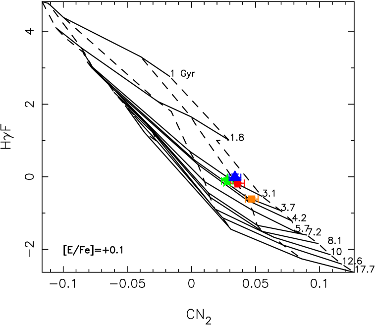
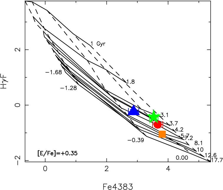
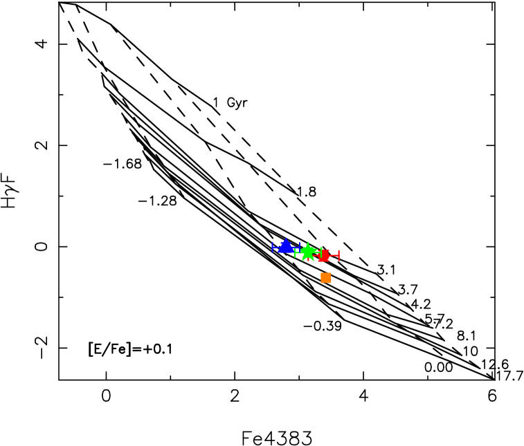
Figure 9: Index-index diagrams for the indices measured in the stacked spectra at different redshifts. Left panels (big symbols) show measurements on the stacked spectra of galaxies with $\sigma$ larger than 175 km s^-1 while right panels (small symbols) show the same measurement for galaxies with $\sigma$ smaller than 175 km s^-1. The different redshifts bins are represented as different colours (and different symbol shapes); $z=0.75$: blue triangles; $z=0.65$: green stars; $z=0.45$: red circles; $z=0.02$: orange squares. Model grids of constant age (solid lines) and constant metallicity (dashed lines) from V08 with [E/Fe]=+0.35 (for the most massive galaxies ) and [E/Fe]=+0.1 (for the lower sigma bins) are superimposed. The ages and metallicities of the different models are indicated in the Figure.

Although the selection of our sample has been done using colours, many previous studies of the red-sequence were restricted to morphologically classified early-type galaxies. To compare with those, the analysis in this section has been repeated for the subset of red-sequence galaxies that are morphologically classified as E or S0 galaxies. For the clusters imaged with the ACS (see Table 1), we use their visual classification (Desai et al. 2007). For the others, we apply the selection criterion of Simard et al. (2008), based on the bulge fraction derived from our VLT I-images (see Sec.9 for the criteria to select early-type galaxies).

The last three rows of Table 6 show the SSP-parameters derived for the red-early-type galaxies. The first thing that can be seen is that the SSP-parameters for the whole red-sequence and for the morphologically classified early-type galaxies are compatible within the errors. Therefore, we will not discuss further the possible differences and will restrict our analysis to the complete red-sequence sample.

	$\sigma>175$ km s-1			$\sigma<175$ km s-1
	Age	[Z/H]	[E/Fe]	Age	[Z/H]	[E/Fe]
	Gyr			Gyr
Coma	$7.90\pm 1.81$	$-0.03\pm 0.06$	$0.40\pm 0.03$	$5.80\pm 0.36$	$-0.11\pm 0.03$	$0.31\pm 0.04$
$z=0.45$	$5.60\pm 1.05$	$-0.01\pm 0.07$	$0.35\pm 0.09$	$3.20\pm 0.64$	$-0.05\pm 0.13$	$0.16\pm 0.12$
$z=0.55$	$3.40\pm 0.52$	$0.11\pm 0.07$	$0.35\pm 0.06$	$3.40\pm 0.81$	$-0.13\pm 0.09$	$0.11\pm 0.13$
$z=0.75$	$2.70\pm 0.38$	$0.18\pm 0.11$	$0.46\pm 0.06$	$3.10\pm 0.83$	$-0.08\pm 0.14$	$0.30\pm 0.21$
$z=0.45$	$5.70\pm 2.42$	$0.02\pm 0.12$	$0.45\pm 0.10$	$2.80\pm 0.46$	$0.01\pm 0.11$	$0.23\pm 0.14$
$z=0.55$	$3.10\pm 0.62$	$0.11\pm 0.12$	$0.30\pm 0.10$	$2.90\pm 0.42$	$-0.04\pm 0.10$	$0.25\pm 0.11$
$z=0.75$	$4.60\pm 2.32$	$-0.07\pm 0.14$	$0.55\pm 0.10$	$2.50\pm 0.34$	$0.11\pm 0.13$	$0.24\pm 0.15$

Table 6: First 4 rows: Ages (measured in Gyr), metallicities [Z/H] and [E/Fe] abundances for the stacked spectra, in different redshift bins, of the red-sequence galaxies, measured using V08 models and the indices H$\gamma_{F}$, Fe4383 and CN₂. The spectra have been stacked separating galaxies with $\sigma$ lower than 175 km s^-1 (right side) and larger than 175 km s^-1 (left side). The parameters have been obtained iteratively as described in the text. Last three rows: Ages, metallicities and [E/Fe] derived for the stacked spectra, at different redshifts, of morphologically classified E and S0 galaxies.

7.1 Massive galaxies

It can be seen in Table 6 and Fig. 9 that the age difference between the redshift bins of the most massive galaxies ($\sigma>175$ kms^-1) corresponds to the expected age difference of the Universe at those redshifts. The absolute age obtained from the models for these galaxies corresponds to a redshift of 1.4. In other words, they are compatible with being formed at $z>1.4$ and evolving passively since then. The metallicity measured from CN₂ does not evolve either, as expected in a passive evolution scheme.

When we look at the panels using Fe4383 instead of CN₂ we can see that the most massive galaxies at $z=0.75$ seem to have a lower Fe4383 than predicted by passive evolution. Jørgensen et al. (2005) similarly found a weaker Fe4383 index for more than half of the galaxies in a sample of red-sequence galaxies (including those with $\sigma$ larger than 175 km s^-1) in the cluster RX J101522.7-1357 at redshift $z=0.83$. This result, if confirmed, could be indicating that at least some massive galaxies have experienced some chemical enrichment since $z=0.75$. It will be necessary to measure other Fe-sensitive indices to confirm this trend. Unfortunately, the wavelength range covered by our spectra does not allow us to do this and, therefore, we will not discuss this further.

7.2 Less-massive galaxies

Contrary to their massive counterparts, galaxies with $\sigma<$ 175 km s^-1 do not show any evolution, within the errors, in age or in metallicity between $z=0.75$ and $z=0.45$. They also evolve less than expected from a pure passive scenario between $z=0.45$ and $z=0.0$. A similar result was reported by Schiavon et al. (2006) with a field galaxy sample. Comparing galaxies from the DEEP2 survey around $z=0.8$ with an SDSS local galaxy sample, they showed that the H$\delta_{F}$ variation was less than predicted by passively evolving models. However, they do not group galaxies by mass. Along the lines discussed by the authors, our results suggest that either individual low-mass galaxies experience continuous low levels of star formation, or that the red-sequence is progressively built-up with new and younger small galaxies. This latter hypothesis is supported by a number of recent works (e.g. Bell et al. 2004; Poggianti et al. 2006; De Lucia et al. 2007; Harker et al. 2006; Faber et al. 2007). This differential evolution for massive and less massive galaxies implies that the mean difference in luminosity-weighted mean-age between massive and intermediate-mass red-sequence galaxies increases with time. This should be taken into account when studying the evolution of the colour-magnitude relation with redshift.

Low-$\sigma$ galaxies show a lower value of [E/Fe] than high-$\sigma$ galaxies, in agreement with the results at low redshift. Most of the $"$enhanced$"$ (E) elements we are considering here arise from massive stars and the bulk of their mass is released in Type II supernova explosions, while at least 2/3 of the Fe is released to the interstellar medium by Type Ia supernovae, with a delay of $\sim$ 1 Gyr. Therefore, the ratio [E/Fe] has classically been used as a cosmic clock to measure the duration of the star formation. The lower [E/Fe] in low-$\sigma$ galaxies can be interpreted as a more extended star formation history, just as found locally.

Table 6 also shows that, within the errors, [Z/H] and [E/Fe] do not vary with redshift for low-$\sigma$ galaxies. Whether galaxies have experienced low-level star formation or new galaxies have entered the red-sequence from the blue cloud, it is still unclear how galaxies that have been forming stars until recently have the same chemical composition as those where star formation was quenched 2 Gyr previously (the lookback time between z$\sim$0.45 and z$\sim$0.75). Answering this question is not trivial, as there are multiple paths by which a galaxy may enter and leave the red-sequence. Furthermore, one has to be careful when interpreting single-stellar population equivalent parameters. While galaxy mean ages are biased towards their last episode of star formation, the chemical composition depends more strongly on the oldest population (see Serra & Trager 2007 for a quantitative study). Therefore, galaxies with different star formation histories can have similar [E/Fe] and [Z/H] if they have formed the bulk of their stars on similar time-scales and with a similar efficiency.

8 Evolution of the index-$\sigma$ relations with redshift

The outcome of the previous section seems to contradict earlier studies, in which the evolution of the index-$\sigma$ relation was found compatible with a high-redshift formation and subsequent passive evolution for all red-sequence galaxies, irrespective of their mass range (Kelson et al. 2001). We will now demonstrate that our index-$\sigma$ relation is also consistent with this scenario, but that this analysis cannot provide robust constraints on the star-formation histories of red galaxies. In fact, the evolution of the index-$\sigma$ relation is also compatible with a more extended star formation history for the intermediate-mass galaxies if the progenitor-bias (i.e. the fact that the galaxies with more extended star formation history (or quenched at later times) drop out of the red-sequence at high redshift van Dokkum et al. (2000)) is taken into account.

Figure 10 displays the relation between H$\gamma_{A}$, H$\gamma_{F}$, CN₂, and Fe4383 and the galaxy velocity dispersion, for the Coma cluster and our EDisCS sample.

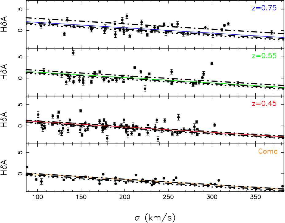
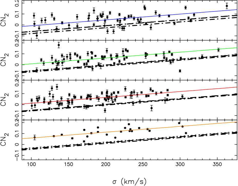
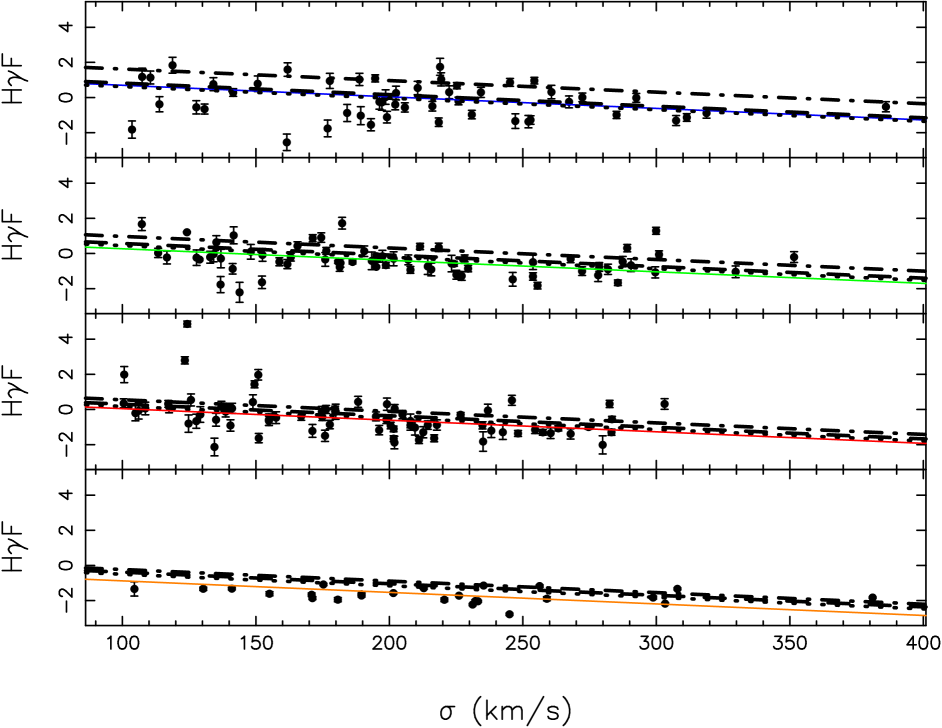
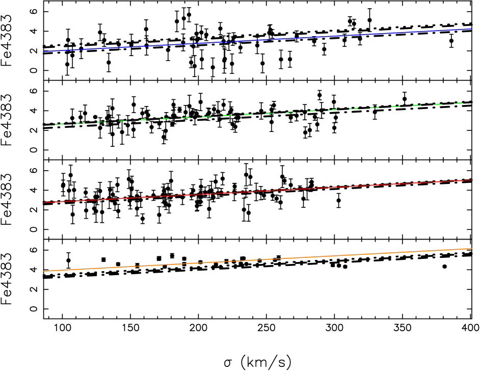
Figure 10: Relation between line-strength indices and the velocity dispersion for the galaxies in the three different bins. Solid coloured lines represent the result of a linear fit to the data forcing the slope to be the same as the one obtained for the galaxies in the redshift bin at $z=0.45$. The black lines represent the expected relation assuming that galaxies formed at $z_{\rm f}$=1.4 (dotted-dashed line), $z_{\rm f}=2$ (thick, dashed line), and $z_{\rm f}$=3 (dotted line), and have evolved passively since then and assigning a solar metallicity for galaxies with velocity dispersion of 300 km s^-1. As can be seen, the evolution of the index-$\sigma$ relation is compatible with a scenario in which the stars formed at $z>1.4$ and evolved passively since then, except for the CN₂ index, which cannot be reproduced by any of the proposed models (see text for details)

. However, the evolution of these relations are also compatible with more complex scenarios (see Sec. 10).

Following Kelson et al. (2001) and Jørgensen et al. (2005), among others, we first calculate the best linear fit to the data using the galaxy sample at $z=0.45$. Then, keeping the slope of the relation fixed, we evolve its zero point with look-back-time. This approach assumes that, if galaxies were coeval and evolving passively, the slope of the relation would not change. In reality, if all the galaxies in the red-sequence were coeval and evolving passively, we would expect a small variation in the slope of the index-$\sigma$ relation, as the variation of the indices is not completely linear with age. However, this variation would be very small over the range of ages considered. To calculate the lines of passive evolution, we used the V08 models, assigning solar metallicity to the galaxies with $\sigma=300$ km s^-1, to match the observed value of the metal-sensitive index Fe4383 at $z=0.45$. We show the best linear fits in Fig. 10, obtained by minimizing the residuals in the $y$-direction. We also show the expected evolution of the index-$\sigma$ relation assuming three different formation redshifts: $z_{\rm f}=$1.4, 2, and $3$. The value $z_{\rm f}=1.4$ is chosen as it corresponds to the mean age measured in the stacked spectra of the massive galaxies in the 0.75 galaxy group (see Sec. 5.2). We only plot models with solar-scaled chemical abundances.

Figure 10 shows that a scenario where all stars form at $z_{\rm f}>1.4$ and evolve passively afterwards is compatible with the observations. The exception is CN₂ which we discuss below. In order to analyze this more quantitatively, we performed a $t-$test, comparing the linear fit values at $\sigma=200$ km s^-1 (which is approximately the mean of the distribution of $\sigma$) with the ones predicted by passive evolution. The results are shown in Table 7. $t$-values higher than 1.9 would indicate that the probability that we have rejected the null-hypothesis (prediction and measurement are equal) by chance is less than $\sim$5%, i.e., a $t$-value higher than 1.9 implies that the passive scenario does not reproduce our relations within the errors. We do not obtain such $t$-values, implying that indeed a passive evolution model can reproduce the evolution of the zero-point of the index-$\sigma$ relations from $z=0$ to, at least, $z$$\sim$0.75. Although we obtain a slightly better agreement between model and data if we assume a formation redshift above $2$, we do not find any statistically significant difference from a formation redshift of 1.4. Noticeably, formation redshifts lower that 1.4 produce an evolution of the index-$\sigma$ relation significantly larger than the one observed.

The relation of the other indices with $\sigma$ is presented in Appendix C. The analysis of these indices gives consistent results without adding any new information to our study, but we show it for comparison purposes with eventual following studies. We did not include CN₂ in the $t$-test procedure as the stellar population models with solar-scaled chemical abundances cannot reproduce the absolute values of this index. This is a well known effect in nearby early type galaxies (Worthey 1998; Sánchez-Blázquez et al. 2003; Kelson et al. 2006; Schiavon et al. 2006; Graves et al. 2007) and it is attributed to differences in the chemical composition of these galaxies compared to the solar values. (Note that in Sect. 5.2 we used models where C/Fe and N/Fe are enhanced with respect to the solar values in order to reproduce this index).

Summarizing, we show here that, in agreement with previous works, the evolution of the index-$\sigma$ relation is compatible with a scenario where the red galaxies formed their stars at z$>$1.4 and have evolved passively since. However, this conclusion has been reached assuming that all red galaxies formed at the same time independently of their mass. The results of Sec. 5.2 argue against this. Furthermore, numerous works (De Lucia et al. 2004, 2007; Kodama et al. 2004) indicate that the red sequence was not yet fully in place at z$\sim$1 and that it has been growing since then. If this effect is taken into account, a more complex star formation history is allowed while keeping the slope and the tightness of the index-$\sigma$ relations. This was proposed by van Dokkum & Franx (2001) to explain the evolution of the magnitude and the constancy and scatter of the colours on the red sequence.

Harker et al. (2006) showed that quenched models, where a constant star formation is truncated at evenly spaced time intervals can explain the evolution of the mean H$\delta$ of all the field red galaxies between $z=1$ to $z=0$. However, they did not explore the dependence of this evolution on galaxy mass. In order to study this aspect, we have used the Bruzual & Charlot (2003) population synthesis models with a Salpeter IMF and solar metallicity. We built a series of star-formation histories starting at z_f=2 where a constant rate of star formation of 1 M_⊙/yr is quenched at different look-back times. Whenever a galaxy satisfies our criteria to belong to the red-sequence, we measure its indices.

Figure 11 shows the resulting line-strength indices assuming 3 different metallicities, $Z=$0.001, 0.004 and 0.02. We display, again, the relation of the indices with $\sigma$ for each redshift bin discussed in Sec. 8. While the index-$\sigma$ relations of the most massive galaxies are only well reproduced by a scenario where star formation is truncated after 1 Gyr (i.e. the rest of the star formation histories produce relations systematically shifted compared to the observed one), less massive ones can be described by a variety of star formation histories, in agreement with our results of Sec. 5.2. Furthermore, this variety of star formation histories is supported by the larger scatter in metallicity and age values at a given mass of low-$\sigma$ galaxies compared to that of the most massive ones (e.g. Concannon et al. 2000). Some studies have claimed that star formation histories of this nature would have problems reproducing the colours of red-sequence galaxies. As a sanity check (see Fig. 12) we verify that these star formation histories reproduce the colours of the red-sequence.

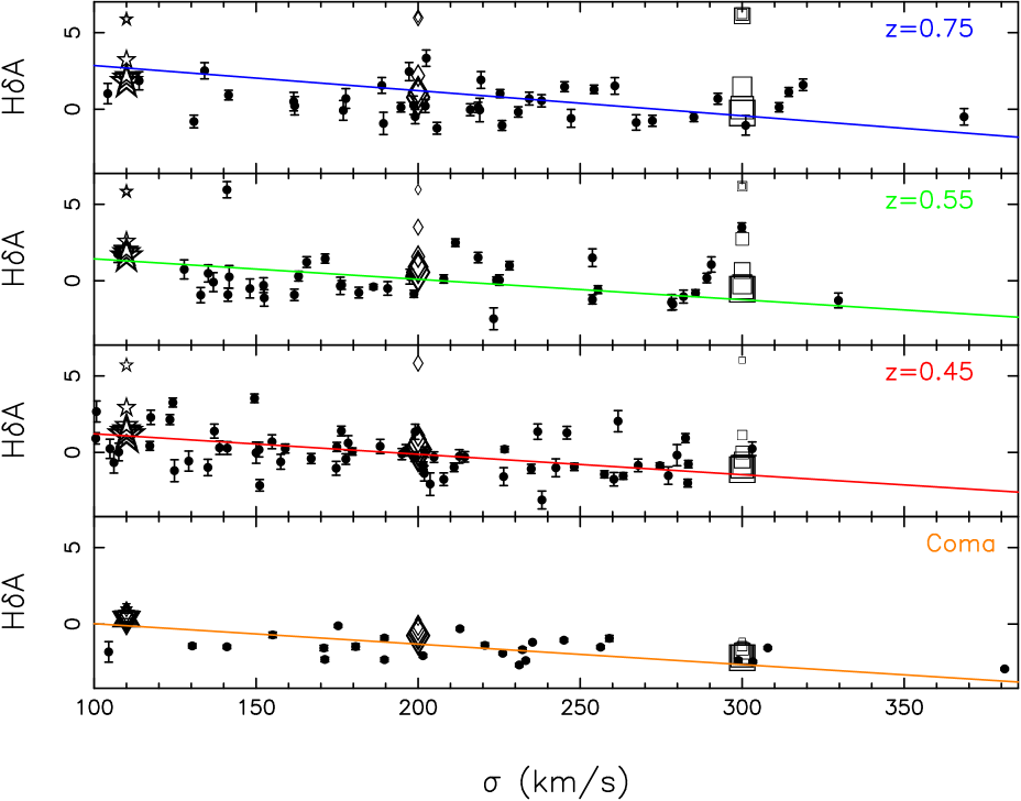
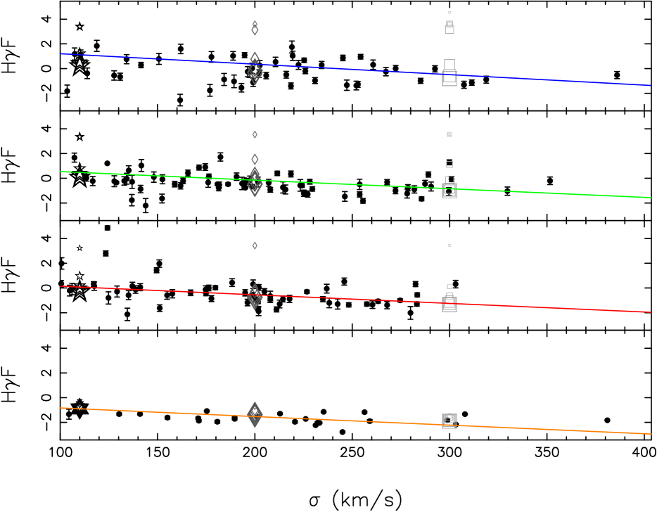
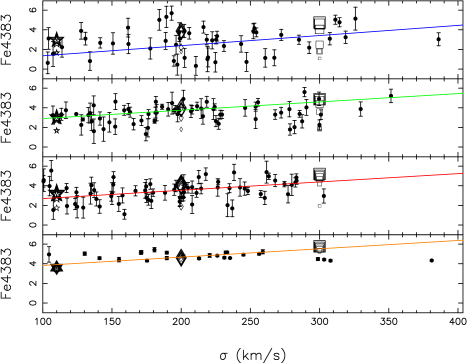
Figure 11: Evolution of the relation of line-strength indices with $\sigma$. We show with coloured, solid lines, the best linear fits to the observations, fixing the slope to that obtained for the redshift bin $z=0.45$ (see Sec. 8). Squares, diamonds, and black stars represent the predicted indices for a constant star formation rate starting at $z_{\rm f}=2$, for stellar populations with metallicities Z=0.001,0.004 and 0.02, respectively. At each of these metallicities, the sta r formation is truncated after 1 (largest symbols), 2, 3, 4 and 5 (smallest symbols) Gyr.

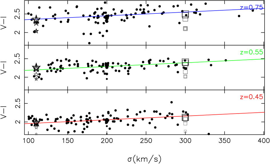
Figure 12: Measured $V-I$ vs $\sigma$ for the galaxies in the different redshift bins. Symbols are the same as in Fig. 11.

This, of course, does not prove that different galaxies have different star formation histories, but it does demonstrate that more complicated scenarios than pure passive evolution are compatible with the index-$\sigma$ relations.

		linear fit		$z_{\rm f}=1.4$		$z_{\rm f}=2$		$z_{\rm f}=3$
Index	redshift	@200 km/s	$\sigma$	@200 km/s	$t$	@200 km/s	$t$	@200 km/s	$t$
Fe4383	0.02	$4.70$	0.41	$4.09$	1.5	$4.33$	0.9	$4.38$	0.8
	0.45	$3.58$	0.82	$3.39$	0.2	$3.57$	0.0	$3.65$	0.1
	0.55	$3.73$	0.38	$3.06$	1.7	$3.40$	0.8	$3.47$	0.8
	0.75	$2.77$	1.24	$2.56$	0.2	$3.19$	0.3	$3.34$	0.4
H$\delta$A	0.02	$-1.40$	0.79	$-1.37$	0.0	$-1.85$	0.6	$-1.93$	0.7
	0.45	$-0.23$	1.12	$-0.08$	0.1	$-0.47$	0.2	$-0.64$	0.4
	0.55	$0.09$	1.09	$0.58$	0.4	$-0.02$	0.1	$-0.26$	0.3
	0.75	$0.63$	1.10	$1.54$	0.8	$0.33$	0.3	$0.05$	0.5
H$\gamma$F	0.02	$-1.48$	0.44	$-0.86$	1.4	$-1.09$	0.9	$-1.13$	0.8
	0.45	$-0.61$	0.66	$0.10$	1.1	$-0.36$	0.4	$-0.48$	0.2
	0.55	$-0.48$	0.66	$0.31$	1.1	$-0.09$	0.6	$-0.21$	0.4
	0.75	$0.04$	0.97	$0.96$	0.9	$0.16$	0.12	$-0.04$	0.0

Table 7: Comparison between the indices predicted by the linear fit to the data at $\sigma=200$ km s^-1 and the ones predicted – at the same velocity dispersion– in a passively evolving model with redshift formations $z_{\rm f}=1.4$, $z_{\rm f}=2$ and $z_{\rm f}=3$. Column 3 shows the predicted value by the linear fit at $\sigma=200$ km s^-1, column 4 the standard deviation among the relation; columns 5, 7 and 9 show the value predicted by the model with redshift formations of 1.4, 2 and 3 respectively. Columns 6, 8 and 10 shows the $t$-parameter of comparing these two values (fitted and predicted) using a Student’s t-test. A $t$ value higher than 1.96 would indicate that the probability that the two values are different by chance is less than 5% (for samples larger than 40 and 6% for smaller samples). As can be seen, none of the values show significant differences from the model.

9 Morphological content of the red-sequence

Table 1 lists the EDisCS structures wich have been observed with the HST/ACS in the F814W band, i.e, all six in the 0.75 redshift bin, six at $z=0.55$, and three at $z=0.45$. In the following, we use the visual classifications of Desai et al. (2007), which has been performed down to $I_{auto}$=23 mag. Since we concentrate on the EDisCS spectroscopic sample, the actual magnitude cuts for the morphological classification are I (r $\leq$ 1$"$) $\sim$ 22 mag at $z=0.45$ and I(r $\leq$ 1$"$) $\sim$ 23 mag at z=0.75. This translates into restframe magnitudes of Mv$\sim-18.7$ and $\sim-$19.3 mag at z=0.45 and z=0.75, respectively. Once we account for the dimming due to passive evolution (0.5 mag from z=0.75 to 0.45 assuming an age of 3.1 Gyr at z=0.75), the intrinsic magnitude cut is the same at all redshifts. We note that some secondary structures at low redshift were discovered in high-redshift targeted fields. Consequently, they were observed down to lower magnitude limits than the primary targets at similar redshifts. As such, they are exceptions to the above general rule. However, they represent a small percentage of the total number of galaxies.

Interestingly, only 15 E/S0 galaxies out of 168 (i.e., 9%) are not on the red-sequence. This is similar to the fraction of blue early-type galaxies found at low redshift (Bamford et al. 2008), which is highly dependent on local density but varies between 12 and 2%.

We concentrate on the N+W red-sequence galaxies, the same for which we have analyzed the stellar population. Figure 13 shows their Hubble type distribution. We also indicate the distribution of galaxies with $\sigma$ $<$ 175km/s. There is no apparent morphological segregation as a function of galaxy mass, i.e, whatever the galaxy mass range, the dominant morphological types on the red-sequence are clearly E and S0, although the entire Hubble sequence is covered.

Figure 13: The distribution of Hubble types among the N+W emission line red-sequence galaxies in redshift bins: E(T=-5), S0(T=$-2$), Sa (T=1), Sab(T=2), Sd(T=7). The solid line histograms trace the morphological distribution for the entire sample. The dashed areas trace the histograms for the galaxies with velocity dispersions lower than 175 km s^-1.

In order to look for possible evolution with time, we now restrict the sample to the EDisCS clusters (galaxy structures with $\sigma$ larger than 400 km s^-1) and fix the area of analysis to the region falling inside a radius of 0.6R₂₀₀ from the cluster centers, where R₂₀₀ is the radius within which the average cluster mass density is equal to 200 times the critical density. R₂₀₀ values were derived using equation (8) in Finn et al. (2005) and are listed in Table 1. These restrictions are governed by the need to have the same spatial coverage in all structures given that a morphology-radius relation is observed in clusters (e.g. Whitmore & Gilmore 1991; Postman et al. 2005). The fraction of galaxies from each morphological type have been corrected for magnitude and spatial incompleteness (Poggianti et al. 2006). Errors in these fractions are calculated using the formulae in Gehrels (1986), since Poissonian and binomial statistics apply to our small samples.

The fraction of early-type galaxies (E and S0) at redshifts $z=0.45$, 0.55 and 0.75 are: 56${}^{+12}_{-13}$%, 61${}^{+9}_{-9}$% and 75${}^{+9}_{-9}$%, respectively. In other words, our calculations suggest that, in the red-sequence, the fraction of early-type galaxies decreases from $z=0.75$ to $z=0.45$.

In order to check the robustness of this result, we also consider another technique of morphological classification. In particular the GIM2D decompositions presented in Simard et al. (2008, in preparation), where early-type galaxies are identified by their bulge fraction ($B/T$$\geq$ 0.35) and the ACS image smoothness within two half-light radii ($S2$ $\leq$ 0.075). This method leads to 33${}^{+14}_{-12}$%, 62${}^{+8}_{-9}$%, and 80${}^{+5}_{-6}$% of early-type galaxies at $z=0.45$,0.55 and 0.75, respectively, in agreement with our previous finding. As mentioned earlier, only 3 clusters have ACS data in the 0.45 bin, and only 22 galaxies within 0.6R₂₀₀, as these clusters did not constitute our primary targets for HST. This most likely explains the large difference found at this redshift between the two classification techniques. Nevertheless, the decrease of early-types fractions in the red-sequence is confirmed. It is worth noting that even when strong emission line galaxies are kept in the sample, the fractions of early-type galaxies are very much the same, i.e., 62${}^{+10}_{-9}$% and 72${}^{+5}_{-7}$% at z=0.55 and z=0.75.

The mean redshift of the MORPHS sample is 0.45 (Dressler et al. 1999), hence allowing direct comparison with our lowest redshift group and increasing the statistical significance (10 clusters). After selection of the red galaxies (g$-$r$>$1.4) without emission lines, i.e, a selection comparable to ours, the fraction of MORPHS E+S0s is 57$\pm$9% (B. Poggianti, private communication), i.e, very close to the initial value coming from our visual classification. Additional evidence of a decrease in early-type fraction with time on the red-sequence comes from Holden et al. (2006) who measured a total fraction of E/S0 galaxies in two clusters at z=0.83 (MS 1054.4–0321 and Cl 0152.7–1357) of 74% and 82%, for their selection in mass ( $>10^{10.9}$ M_⊙ ), best corresponding to our red-sequence criteria. Note that our selection extends to lower masses or accordingly to fainter limits, i.e., $3-6\times 10^{10}$ M_⊙ (derived from stellar M/L with the calibration by Bell & de Jong (2001) and the re-normalization proposed by de Jong & Bell (2007) for elliptical galaxies). However, in this fainter regime, Holden et al. take into account all cluster galaxies, rather than only those on the red-sequence, making impossible a direct comparison. Anyhow, their figure 2 shows that their early type fraction can not vary much along the red-sequence. Figure 14 summarizes our results.

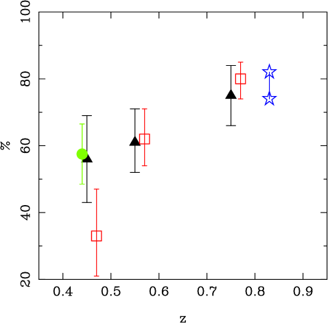
Figure 14: Variation of the fraction of early-type galaxies in the red-sequence with redshift. Black and red symbols show the fraction derived from the EDisCS data. Black triangles show the results for the morphological classification based on visual inspection. Red squares stand for the GIM2D bulge and disk decomposition method, where early-type galaxies are selected upon their bulge-to-total light fractions and image smoothness. The green circle represents MORPHS and the blue star indicates the results of Holden et al. (2006), for their two X-ray selected clusters.

The decrease, on the red-sequence, of the early-type fraction represents a remarkable synthesis between the results of Desai et al. (2007) who detect no evolution in the cluster total fraction of E/S0 galaxies between redshift 0.4 and 1.4, and those of De Lucia et al. (2007) who measure a decrease of the red-sequence faint-to-luminous galaxy ratio of $\sim$40 % between redshift 0.45 and 0.75. Indeed, if the red-sequence keeps building up, as suggested by De Lucia et al. (2007), it must find its supply in the cluster blue galaxies. These EDisCS blue galaxies are composed of only 20$\pm$7% early-types and of 80% spiral galaxies. This distribution in types is constant with redshift. Hence, provided that galaxy colours redden before any morphological transformation occurs, an increase in the number of spirals on the red-sequence is naturally expected when new galaxies reach it. By restricting our analysis to the EDisCS spectroscopic sample, we do not reach as faint magnitudes as De Lucia et al. (2007). As a consequence, our 20% variation in the fraction of E/S0 galaxies on the red-sequence between redshifts 0.45 and 0.75 most certainly constitutes a lower limit.

It is interesting to estimate the subsequent evolution of the red-sequence population, i.e., from $z=0.45$ to $z=0$. Dressler et al. (1997) and Fasano et al. (2000) found that, while the elliptical fraction does not evolve in the redshift range 0.5 to 0.0, the fraction of lenticular galaxies doubles. This increase in the number of S0s is accompanied by a drop in the fraction of (Sp+Irr) type galaxies. Combining these results together with those of Postman et al. (2005) and EDisCS, Desai et al. (2007) conclude that $z\sim 0.4$ must constitute a special epoch after which the total fraction of S0-type galaxies in clusters begins to increase. Meanwhile, De Lucia et al. (2007) measure only $\sim 10$ % variation of the red-sequence faint-to-luminous galaxy ratio between redshift 0.45 and 0. As a consequence, at the time the red sequence reduces its growth ($z\leq 0.45$), one can expect a rise in its E/S0 fraction as well.

10 Discussion

We have shown that the rate at which red-sequence galaxies evolve depends on their mass range. In particular, less massive galaxies show evidence for a more extended star formation history. Two possibilities are considered: i) the sequence is in place at redshift $z\sim 0.8$, but a low level of star formation continues in galaxies on the faint end (e.g. Chiosi & Carraro 2002); or ii) the red-sequence is continuously built-up by new incomers, preferentially selected among faint systems. We examine both hypotheses.

Gebhardt et al. (2003) explore, in the context of the first model, the maximum amount of low-level star formation that the galaxies can experience without leaving the red-sequence. They found that, to keep the colours of the red-sequence galaxies almost constant since $z=1$, in agreement with observations, only 7% of the mass could have been formed after the initial burst (assumed to be at $z=$1.5) using exponential star formation histories with e-folded time of 5 Gyr. We did a similar experiment, and calculated the maximum amount of low-level star formation that the galaxies could experience from $z=0.75$ to $z=0.45$ in order to reproduce the evolution of the index-$\sigma$ relations with redshift measured in Sect. 8. The exact percentage depends on the chosen metallicity but we also find that this fraction has to be always less than $\sim$10% (note that our redshift baseline is smaller). However, recent results of the evolution of the UV colours in early-type galaxies suggest that this percentage is higher: Kaviraj (2008) found that, at intermediate luminosity (M${}_{\rm v}<-20.5$), early-type galaxies in the red-sequence have formed 30-60% of their mass since $z=1$. However, this study does not sample exclusively galaxies in dense clusters, but in a wide range of different environments.

Faber et al. (2007); Poggianti et al. (2006) proposed a mixed scenario where red-sequence galaxies form through by two different channels. Poggianti et al. (2006) discussed a scenario where the red-sequence is composed of primordial galaxies formed at $z_{\rm f}>$2.5 on the one hand and of galaxies that quenched their star formation due to the dense environment of clusters on the other hand. They calculate that, of the 80% of passive galaxies at z=0, 20% are primordial and 60% have been quenched. With regards to this later aspect, Harker et al. (2006) could reproduce the evolution of $U-B$ and the H$\delta$, as well as the galaxy number density, by assuming models of constant star formation histories truncated at evenly spaced intervals of 250 Myr up to now.

Along this line, we calculate the number of new quenched galaxies that have to enter the red sequence to reproduce the results obtained in Sec. 5.2. We start with a population of galaxies with a formation redshift of $z_{f}=1.4$ and solar metallicity, both derived for the low-mass galaxy bin at $z=0.75$. Then we consider galaxies that started forming stars at $z=2$ at a constant rate of 1M_⊙/yr and start quenching them at regular intervals of 250 Myr. Once a galaxy is red enough to pass our red-sequence selection criteria at $z=0.45$ and 0.55, we add its normalized spectrum to the that of the initial population. If we assume that all the new galaxies have velocity dispersions lower than 175 km s^-1, we need $\sim$40% of new arrivals in the interval z=0.75 to z=0.45 in order to reproduce the constant luminosity-weighted age of the low-$\sigma$ galaxy bins with redshift. This is in surprisingly exact correspondence with the result of De Lucia et al. (2007), who measure a decrease of the red-sequence faint-to-luminous galaxy ratio of $\sim$40 % between redshifts 0.45 and 0.75. Note that De Lucia et al. (2007) deal with photometric data and therefore their dataset reaches fainter magnitudes than our spectroscopic sample. The exercise presented here is of extremely simple nature and is not intended to represent the true star formation histories of the galaxies. Apart form quenching, disk galaxies can merge and have bursts of star formation before becoming red. By merging with other galaxies, our objects can also move from the low-$\sigma$ bin to the high-$\sigma$ bin, which is something not considered here. However, simple models similar to this one have proved to be very successful in reproducing the evolution of the colours and H$\delta$ index and the evolution of the luminosity function (e.g., Harker et al. 2007).

Linking these constraints to our morphological results, it appears that the mechanism that quenches star formation does not necessarily produce a morphological transformation at the same time, but certainly, it favors it. Most likely, the mechanism that quenches star formation also produces the morphological transformation, but on a different time-scale. Indeed, the fraction of spiral galaxies evolves by 20% and not by the 40% calculated in the spectroscopic analysis. Splitting between stellar population and morphologies was also raised by MORPHS (Dressler et al. 1999; Poggianti et al. 1999).

11 Summary

We addressed the questions of the epoch of formation of the reddest galaxies in clusters, the extent of their period of star formation and the link between morphological and stellar population evolution time scales.

Our analyses are primarily based on 215 red-sequence galaxies, selected from the EDisCS spectroscopic database, that we divided into three redshift bins, $z=0.75$, $0.55$, and $0.45$. We considered their mass range, via the proxy of their velocity dispersions; their stellar population properties derived from absorption line features; and their morphologies, thanks to HST/ACS imaging. We have been able to trace the evolution of the red-sequence from $z=0.75$ to $z=0.45$ in a homogeneous dataset, the largest to date, extracted from a single survey, hence avoiding a mix of different systematic errors.

$\bullet$ Before discarding red-sequence galaxies with strong emission lines from our absorption line analysis, we investigated the nature of their ionizing sources. Most of the EDisCS red-sequence galaxies with emission lines seem to be forming stars. The proportion of dusty star forming galaxies among our total sample is larger than the fraction reported by Yan et al. (2006) at $z=0$ in the SDSS field red population. Whether this difference is due to evolution or to environment is worth clarifying in the future.

$\bullet$ We measured 12 Lick/IDS indices, carefully visually inspecting the spectra in order to eliminate those possibly affected by sky subtraction residuals or any other systematic effect. To compare with our local sample of Coma galaxies, we derived new aperture corrections. We used state-of-the art stellar population models to derive ages, metallicities, and chemical abundance ratios. These models make predictions over the whole spectral energy distribution, allowing us to analyze our data at a resolution of 325 km/s, avoiding any spurious correction for the galaxy velocity dispersion.

$\bullet$ After selecting on secure redshifts and signal-to-noise ratios, we stacked the galaxy spectra in redshift bins. In each bin, we also distinguished galaxies with respect to their velocity dispersions, dividing at $\sigma=175$ km s^-1. We derived the age, metallicity (Z), and $\alpha$-element abundance ([E/Fe]) of each redshift and velocity dispersion group.

• Massive galaxies ( $\sigma>175$ km s^-1 ) show a variation in age corresponding to the expected cosmological variation between redshifts, a mean solar metallicity and an overabundance [E/Fe] with respect to the solar values. Therefore, they are well represented by a scenario of formation at high redshift, followed by passive evolution. Conversely, the properties of less massive galaxies ($\sigma<175$ kms^-1) require longer star formation, at low level. Indeed, their luminosity weighted ages is found constant with time in our redshift range. An immediate consequence is that the age difference between low- and high-$\sigma$ galaxies increases with time. This need to be taken into account in studies of the evolution of the colour-magnitude diagrams.

• Values of [E/Fe] and [Z/H] are constant with time, independent of $\sigma$. This implies that the bulk of the galaxy stellar population is formed on a time-scale and with efficiency fixed by the galaxy mass. Possible subsequent episodes of star formation, which change the age of the less-massive galaxies, can not account for a large fraction of the galaxy mass.

$\bullet$ We confirm that the evolution of the zero-points of the index-$\sigma$ relationships with redshift is compatible with a scenario in which galaxies formed all their stars at high redshift and evolved passively since then. However, we demonstrate that it is also compatible with more complex star formation histories. In particular, galaxies can progressively enter the red-sequence as their star formation is quenched. In this scenario, galaxies with lower $\sigma$ enter the red-sequence at lower redshift than more massive galaxies.

The two more important results of this work are:

$\bullet$ The morphological analysis, based on visual or automated classification, indicates that red sequences are composed of types covering the entire Hubble sequence, irrespective of the redshift, with, however, a very clear plurality of Es and S0s. The fraction of red-sequence early type galaxies decreases between $z=0.75$ and $z=0.45$ by about 20%. This means that spiral galaxies get first redder, stopping their star formation, before they turn into earlier morphological types. This evolution is however lower than the rate at which new galaxies enter the red-sequence, meaning that quenching and morphological transformation operate on different time-scales.

$\bullet$ We found that the evolution of the line-strength indices with redshift can be reproduced if 40% of the galaxies with $\sigma$ lower than 175 kms^-1 entered the red-sequence between $z=0.75$ and $z=0.45$, in agreement with the fraction derived in studies of the luminosity function.

In summary, a number of works dedicated to the evolution of the luminosity function of red galaxies in clusters (Rudnick et al. 2008, in preparation; De Lucia et al. 2004; De Lucia et al. 2007) and in the field (Faber et al. 2007; Brown et al. 2007) report an increase of the galaxy number density since $z\sim$1. Conversely, colour-magnitude diagrams and index-$\sigma$ relations of cluster red-sequence galaxies at intermediate- and high-redshift usually describe them as in place very early, passively evolving, independently of their mass (e.g., Ellis et al. 1997; Dressler et al. 1997; van Dokkum et al. 1998; Stanford et al. 1998; Kelson et al. 2000; Ziegler et al. 2001; Blakeslee et al. 2003; Wuyts et al. 2004; Tran et al. 2007). The present work reconciles the luminosity functions and stellar content outcomes.

Appendix A Transformation to the Lick system

Although the new generation of stellar population models is starting to make predictions, not only of individual features, but of the whole spectral energy distribution (e.g. Vazdekis 1999; Vazdekis et al. 2003; Bruzual & Charlot 2003), some of the most popular ones (e.g. Worthey 1994; Thomas et al. 2003) still base their predictions on the original fitting functions released by the Lick group (Gorgas et al. 1993; Worthey et al. 1994). In order to compare with these models and with the bulk of the data in the literature, which is usually transformed onto this system, one has to follow two steps. The first step is to degrade the resolution of the spectra into the wavelength variable resolution of the Lick system (Worthey & Ottaviani 1997, see) and then apply a correction due to the velocity dispersion of the galaxies. The second step is to correct small systematic differences in the indices due to differences in the shape of the spectra of the Lick/IDS stars and a fully-flux calibrated spectrum. To do that, one usually observes stars in common with the Lick library with the same instrumental configuration as the objects one wants to analyze and compare the indices after degrading their spectra to the Lick resolution. This cannot be done, though, in the growing number of work analyzing Lick indices in galaxies at high redshift. For these cases when stars in common with Lick are not present, it is still possible to correct for the instrumental response of the Lick/IDS stars by applying an offset derived by comparing flux calibrated spectra with Lick/IDS spectra previously degraded to the Lick/IDS resolution. This experiment has been attempted before by Worthey & Ottaviani (1997) and Bruzual & Charlot (2003) using the Jones (1999) and STELIB (Le Borgne et al. 2003) libraries respectively. Here we present new offsets using the MILES library (Sánchez-Blázquez et al. 2006c). The advantage of this calibration is that the MILES library contains a large number of stars (242) in common with the Lick/IDs library. Furthermore, the flux calibration is very accurate (better than 1%)

To obtain the offsets we broadened the MILES spectra to the wavelength-dependent resolution of the Lick/IDS spectra using figure 7 in Worthey & Ottaviani (1997) and measured the Lick/IDS indices with the definition given in Trager et al. (1998). In some cases, differences between the indices measured in both datasets can be described with a linear fit, better than with a single offset. Therefore, we have also derived a linear transformation between both libraries obtained with a simple linear regression eliminating galaxies deviating more than 3 times the rms from the relation.

Index	offset	Linear relation
	(MILES-Lick)	(MILES=a+ b $\times$ Lick)
CN1	$0.007$	$0.0082(0.0017)+0.9112(0.0124)$
CN2	$0.006$	$0.0101(0.0021)+0.9040(0.0136)$
Ca4227	$-0.081$	$0.0627(0.0256)+0.9046(0.0119)$
G4300	$-0.032$	$0.5795(0.0663)+0.8480(0.0126)$
Fe4383	$-0.587$	$-0.1660(0.0798)+0.9321(0.0154)$
Ca4455	$-0.391$	$-0.0752(0.0340)+0.7849(0.0204)$
Fe4531	$-0.109$	$0.3201(0.0544)+0.8541(0.0164)$
Fe4668	$0.050$	$0.5664(0.0649)+0.8873(0.0110)$
H$\beta$	$0.068$	$0.1535(0.0283)+0.9755(0.0108)$
Fe5015	$-0.629$	$0.1940(0.0543)+0.8573(0.0088)$
Mg1	$-0.005$	$-0.0024(0.0001)+0.9263(0.0082)$
Mg2	$-0.020$	$-0.0043(0.0012)+0.9186(0.0050)$
Mgb	$-0.208$	$0.2201(0.0351)+0.8934(0.0089)$
Fe5270	$-0.151$	$0.1311(0.0393)+0.9008(0.0147)$
Fe5335	$-0.060$	$0.1059(0.0361)+0.9268(0.0150)$
Fe5406	$0.045$	$0.2190(0.0242)+0.8543(0.0151)$
Fe5709	$-0.029$	$0.0135(0.0227)+0.9162(0.0242)$
Fe5782	$-0.029$	$0.0157(0.0208)+0.9361(0.0267)$
Na5895	$-0.148$	$-0.1842(0.0352)+1.0038(0.0107)$
TiO1	$-0.014$	$-0.0066(0.0006)+0.9128(0.0065)$
TiO2	$-0.010$	$0.0015(0.0007)+0.9119(0.0045)$
H$\delta_{A}$	$0.083$	$0.0286(0.0512)+0.9354(0.0115)$
H$\gamma_{A}$	$-0.073$	$-0.2029(0.0565)+0.9607(0.0082)$
H$\delta_{F}$	$-0.013$	$0.0069(0.0329)+0.9585(0.0147)$
H$\gamma_{F}$	$-0.051$	$-0.0750(0.0258)+0.9763(0.0091)$

Table 8: Mean index offsets between he stars in common between MILES and the Lick/IDS. Some times the differences can be better described with a linear relation than a simple offset. Last column display the best linear relation describing the relation of the indices measured in MILES and Lick/IDS spectra.

In principle, the offsets between the indices measured in the Lick and other libraries are due to differences in the continuum shape. However, as was noted before by Worthey & Ottaviani (1997), some of the indices with larger differences have very narrow definition bands and show a very small dependence with the flux shape. Therefore, the reason for the differences is not clear.

The mean offsets and linear relations obtained in the comparison between the MILES and Lick/IDS libraries are listed in Table 8.

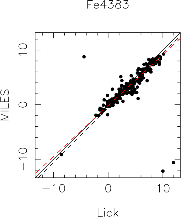
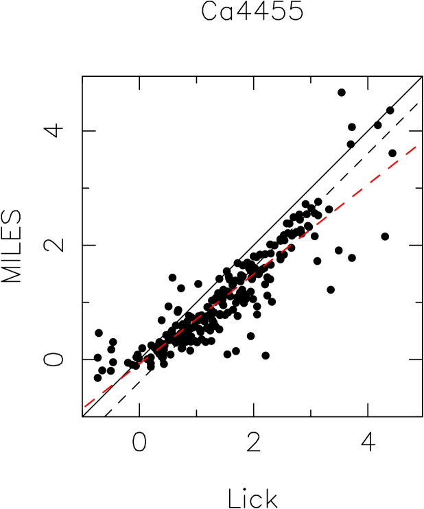
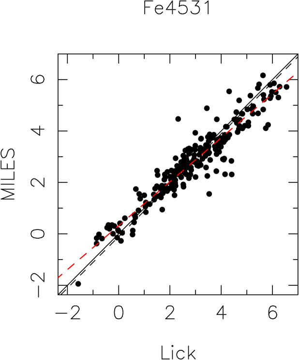
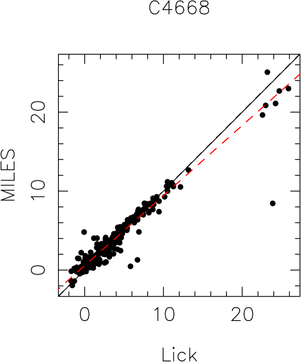
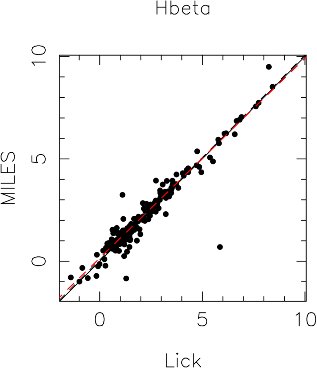
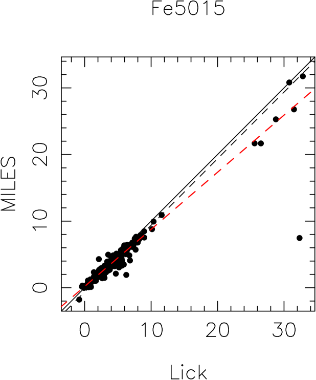
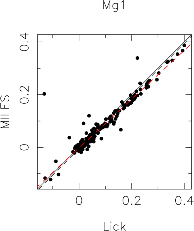
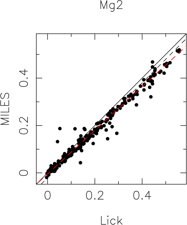
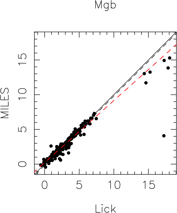
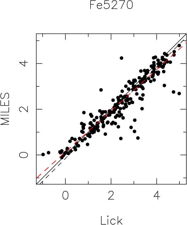
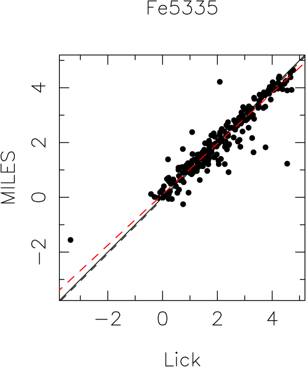
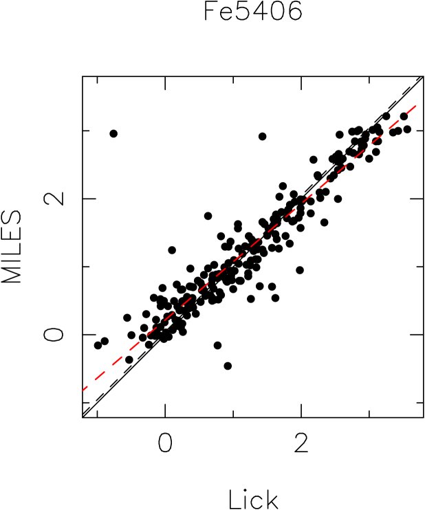
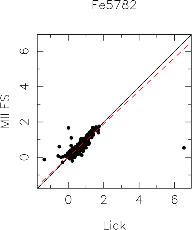
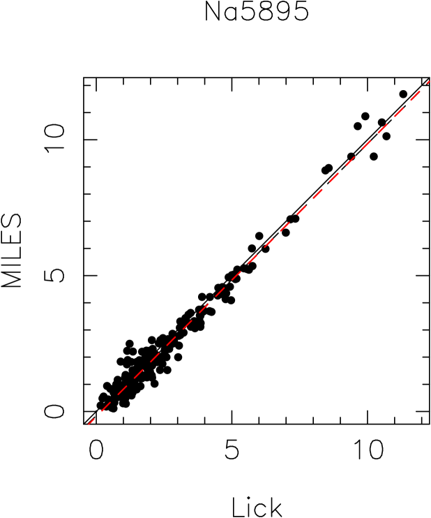
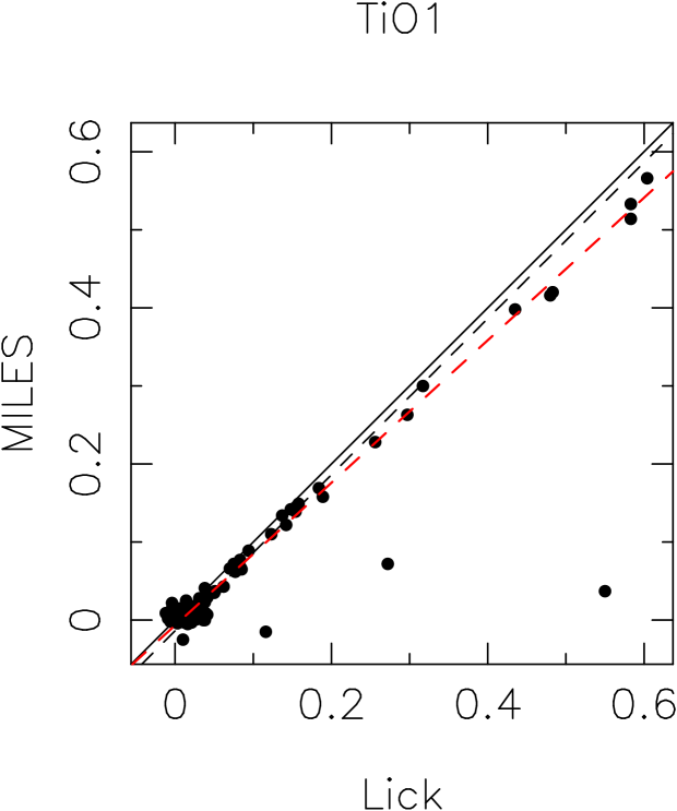
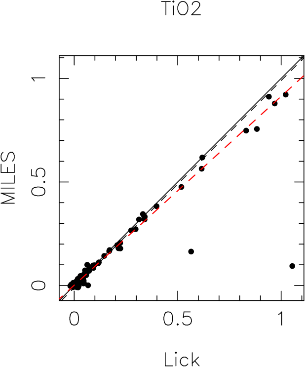
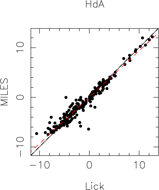
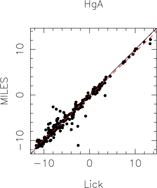
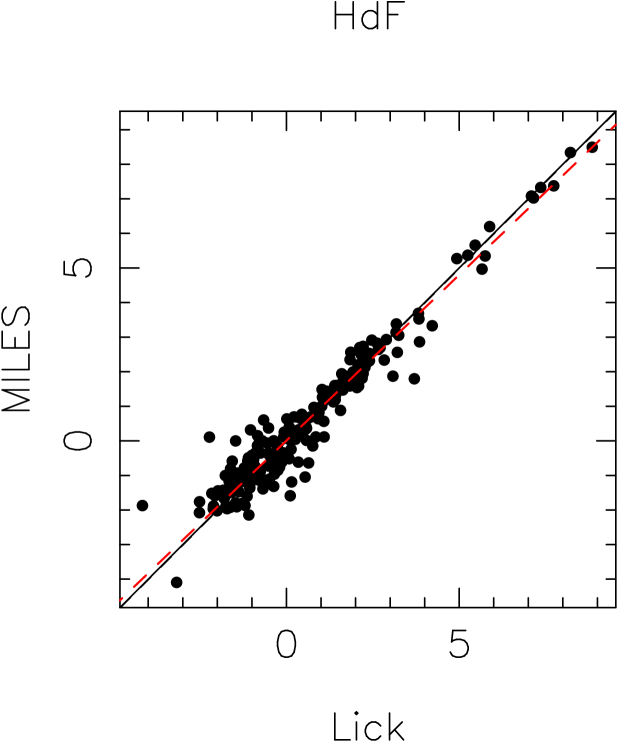
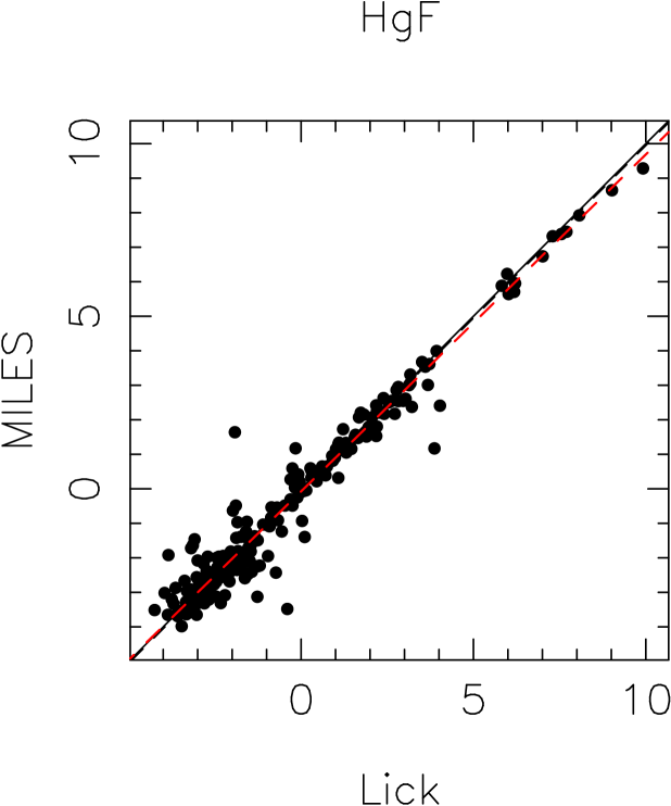
Figure 15: Comparison between the Lick/IDS indices measured in the stars in common between the MILES and Lick/IDS libraries. The solid line represents the 1:1 relation. The dashed line shows the calculated offset, while the red dashed line indicates the best linear fit to the data.

Appendix B Mean gradients and aperture correction

Galaxies have radial gradients in the line-strength indices and, therefore, when comparing galaxies at different redshifts, the indices need to be aperture corrected. Jørgensen (1997) and Jørgensen et al. (2005) present a series of corrections based on the radial gradients from Vazdekis et al. (1997), Cardiel et al. (1998), and Davidge & Clark (1994). However, those works do not include many of the Lick indices, particularly the higher order Balmer lines.

We have derived new aperture corrections for all the Lick/IDS indices + the higher order Balmer line indices (Worthey & Ottaviani 1997), taking advantage of the large sample of nearby galaxies presented in Sánchez-Blázquez et al. (2006a) and Sánchez-Blázquez et al. (2007). To calculate the $\alpha$ parameter, we assume that the light in our galaxies follows a de Vaucouleur profile. Using the gradients for each individual galaxy, we obtain the final index inside an aperture as the luminosity-weighted index. We then calculate how the final indices depends on aperture size. The variation of the luminosity-weighted indices with different aperture sizes can be described as power law. Therefore, aperture corrections (those measured in Å) can be written as (see Jørgensen et al. 1995; Jørgensen 1997):

$$\log(index)_{corr}=\log(index)_{ap}+\alpha\log\frac{r_{ap}}{r_{nor}},$$ (2)

and for molecular indices and higher-order Balmer lines:

$$index_{corr}=index_{ap}+\alpha\log\frac{r_{ap}}{r_{nor}},$$ (3)

where $r_{ap}$ is the equivalent circular aperture, obtained as $2r_{ap}=1.025\times 2(xy/\pi)^{1/2}$; and $x$ and $y$ are the width and the length of the rectangular aperture.

The $\alpha$ coefficients are listed in Table 9 and can be used by any other study. In our case, we were more interested in selecting a fraction of the total light of the galaxy instead of a fixed aperture and therefore $y$ is not fixed but is chosen to be a FWHM of the spatial profile. However, we have fixed the $y$ for all the spectra to be the physical aperture equivalent to 1 arcsec (the width of the slit) at $z=0.75$. The correction for the galaxies at $z>$ 0.4 was very small and we did not apply any. The aperture correction was applied only to the galaxies in the Coma cluster.

Elliptical galaxies show a great variety of gradients that do not seem to be correlated with any other properties of the galaxies, like mass or colour. For this reason, we used the mean gradient to compute the aperture corrections. We calculated an error due to the dispersion among the mean of all the measured gradients. To do this, we performed a series of Monte Carlo simulations where each gradient was perturbed following a Gaussian distribution with $\sigma$ equal to the typical RMS dispersion in the gradients. For each new gradient, the coefficient $\alpha$ and the final correction for the galaxies in the Coma cluster were recomputed. The errors in the aperture correction calculated this way are indicated in Table 4.

Index	$\alpha$	Type
$\sigma$	$0.058\pm 0.047$	1
D4000	$0.027\pm 0.018$	1
H$\delta_{A}$	$-0.721\pm 0.508$	2
H$\delta_{F}$	$-0.206\pm 0.249$	2
CN1	$0.058\pm 0.023$	2
CN2	$0.059\pm 0.030$	2
Ca4227	$0.047\pm 0.075$	1
G4300	$0.027\pm 0.022$	1
H$\gamma_{A}$	$-0.850\pm 0.422$	2
H$\gamma_{F}$	$-0.436\pm 0.321$	2
Fe4383	$0.061\pm 0.033$	1
Ca4455	$0.097\pm 0.075$	1
Fe4531	$0.040\pm 0.021$	1
Fe4668	$0.119\pm 0.049$	1
Fe5015	$0.05\pm 0.02$	1
H$\beta$	$-0.05\pm 0.19$	1
Mgb	$0.048\pm 0.051$	1

Table 9: $\alpha$ coefficient and corresponding error obtained using the samples of SB06 and Sánchez-Blázquez et al. 2007.

Appendix C Relation of the Lick/IDS indices with velocity dispersion

Figure 10 shows the relation between all the measured line-strength indices and the velocity dispersion for the 4 considered redshift bins.

		linear fit		$z_{\rm f}=1.4$		$z_{\rm f}=2$		$z_{\rm f}=3$
Index	redshift	@200 km s-1	$\sigma$	@200 km s-1	$t$	@200 km s${-1}$	$t$	@200 km s-1	$t$
D4000	0.45	2.03	0.11	1.94	0.8	1.98	0.4	2.01	0.2
	0.55	2.08	0.07	1.85	3.2	1.93	2.1	1.96	1.7
	0.75	1.98	0.12	1.75	1.9	1.89	0.7	1.92	0.5
	0.02	2.12	0.12	2.11	0.1	2.16	0.3	2.20	0.7
H$\delta_{F}$	0.45	0.92	0.52	1.05	0.2	0.86	0.1	0.79	0.2
	0.55	0.99	0.89	1.36	0.4	1.07	0.1	0.97	0.0
	0.75	1.40	0.71	1.80	0.6	1.24	0.2	1.10	0.4
	0.02	0.70	0.33	0.50	0.6	0.38	0.9	0.28	1.3
Ca4227	0.45	0.82	0.31	1.06	0.8	1.12	0.9	1.15	1.1
	0.55	0.89	0.27	0.97	0.3	1.05	0.6	1.08	0.7
	0.75	0.83	0.32	0.86	0.1	0.99	0.5	1.05	0.7
	0.02	1.17	0.16	1.27	0.6	1.33	1.0	1.39	1.3
G4300	0.45	4.58	0.81	3.87	0.9	4.03	0.7	4.12	0.6
	0.55	4.41	0.53	3.55	1.6	3.85	1.0	3.95	0.8
	0.75	4.06	1.31	3.05	0.8	3.66	0.3	3.81	0.2
	0.02	5.25	0.51	4.35	1.7	4.41	1.6	4.45	1.5
Ca4455	0.45	0.86	0.28	0.88	0.1	0.91	0.2	0.91	0.2
	0.55	0.96	0.30	0.83	0.4	0.88	0.3	0.90	0.2
	0.75	0.79	0.61	0.75	0.1	0.85	0.1	0.87	0.1
	0.02	1.15	0.12	0.97	1.5	1.00	1.2	1.02	1.1
Fe4531	0.45	2.77	0.43	2.76	0.0	2.82	0.1	2.83	0.1
	0.55	2.93	1.74	2.66	0.1	2.75	0.1	2.78	0.1
	0.75	2.51	0.80	2.53	0.0	2.69	0.2	2.74	0.3
	0.02	3.04	0.23	2.92	0.5	2.98	0.3	3.03	0.0
H$\gamma_{A}$	0.45	$-3.85$	1.35	$-2.92$	0.7	$-3.38$	0.3	$-3.61$	0.2
	0.55	$-3.83$	1.77	$-2.12$	0.9	$-2.89$	0.7	$-3.12$	0.4
	0.75	$-2.56$	1.87	$-0.86$	0.9	$-2.41$	0.1	$-2.78$	0.1
	0.02	$-5.56$	1.04	$-4.38$	1.1	$-4.68$	0.8	$-4.90$	0.6

Table 10: Comparison between the indices predicted by the linear fit to the data at $\sigma=200$ km s^-1 and the ones predicted – at the same velocity dispersion – in a passively evolving model with formation redshifts of $z_{\rm f}=1.4$, $z_{\rm f}=2$ and $z_{\rm f}=3$. Column 3 shows the value predicted by the linear fit at $\sigma=200$ km s^-1; Column 4 shows the standard deviation of the relation; Column5 shows the value predicted by the SSP model; and the last column shows the $t$ parameter of the comparison of these two values. A $t$ value higher than 1.9 would indicate that the there is a 5% probability that the two values are different by chance. As can be seen, none of the values show significant differences from the model.

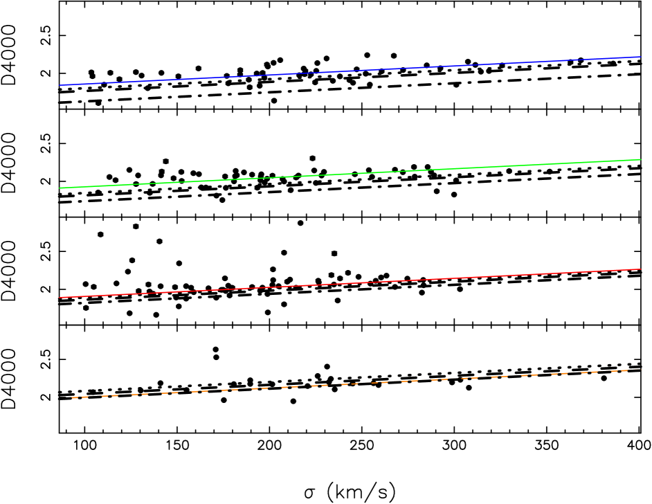
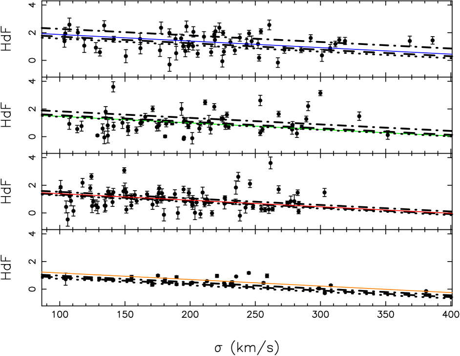
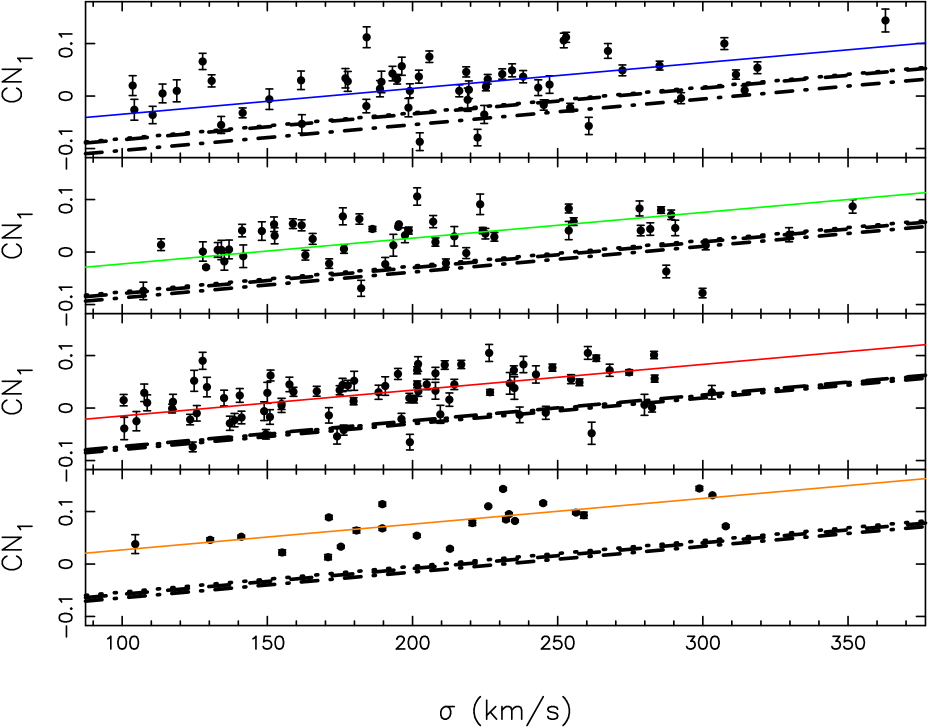
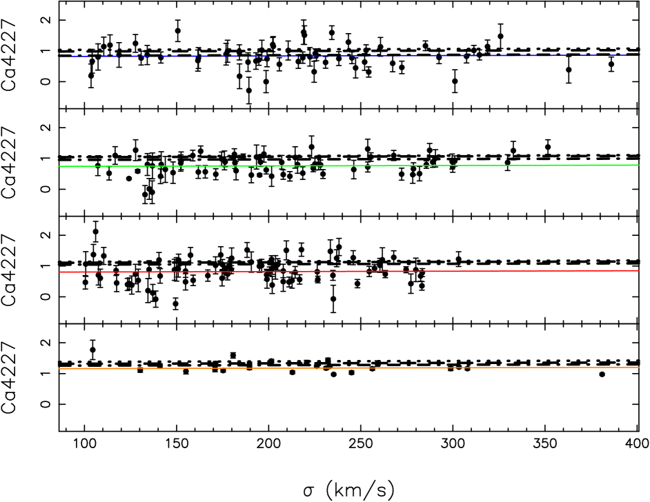
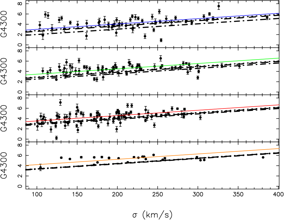
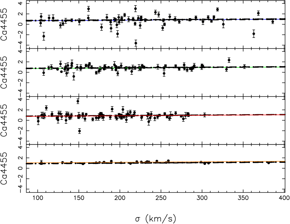
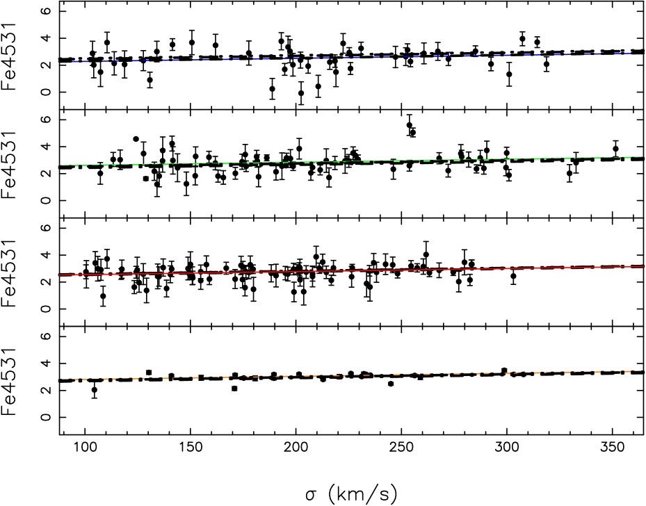
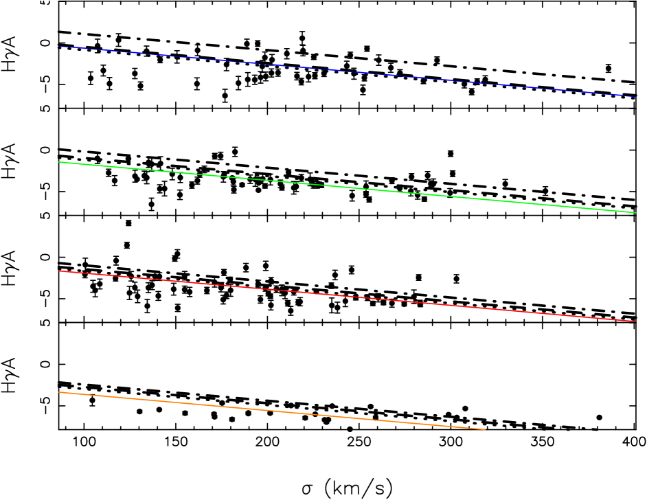
Figure 16: Relation of the indices with the velocity dispersion for the galaxies of the sample grouped in three different redshift bins. The meaning of the lines is the same as in Fig. 10. From top to bottom: $z=0.75$, $z=0.55$, $z=0.45$, and Coma galaxies are represented.