The broad H$\alpha$, [O iii] line wings in stellar supercluster A of NGC 2363 and the turbulent mixing layer hypothesis

Abstract

Context. Supercluster A in the extragalactic H ii region NGC 2363 is remarkable for the hypersonic gas seen as faint extended broad emission lines with a full-width zero intensity of 7000 ${\rm km\,s^{-1}}$.

Aims. We explore the possibility that the observed broad profiles are the result of the interaction of a high-velocity cluster wind with dense photoionized clumps.

Methods. The geometry considered is that of near static photoionized condensations at the surface of which turbulent mixing layers arise as a result of the interaction with the hot wind. The approximative treatment of turbulence was carried out using the mixing length approach of Cantó& Raga. The code mappings ic was used to derive the mean quantities describing the flow and to compute the line emissivities within the turbulent layers. The velocity projection in three dimensions of the line sources was carried out analytically.

Results. A fast entraining wind of up to $\approx 4300\,$${\rm km\,s^{-1}}$ appears to be required to reproduce the faint wings of the broad H$\alpha$ and [O iii] profiles. A slower wind of 3500 ${\rm km\,s^{-1}}$, however, can still reproduce the bulk of the broad component and does provide a better fit than an ad hoc Gaussian profile.

Conclusions. Radial acceleration in 3D (away from supercluster A) of the emission gas provides a reasonable first-order fit to the broad line component. No broad component is predicted for the [N ii] and [S ii] lines, as observed. The wind velocity required is uncomfortably high and alternative processes that would provide comparable constant acceleration of the emission gas up to 4000 ${\rm km\,s^{-1}}$ might have to be considered.

1 Introduction

NGC 2363, the largest and most massive H ii region in the dwarf galaxy NGC 2366 (distance = 3.42 Mpc; Thuan & Izotov 2005) harbors one of the best documented cases of hypersonic gas seen as faint extended broad emission lines in an increasing number of giant extragalactic H ii regions (Tenorio-Tagle et al. 1997; Westmoquette et al. 2007a,b,c, 2008). In NGC 2363, this broad component, first reported by Roy et al. (1992), appears as a faint pedestal under the narrow H$\alpha$, H$\beta$ and [O iii] lines of the so-called knot A (Gonzalez-Delgado et al. 1994). This pedestal has an fwhm in excess of 2300 ${\rm km\,s^{-1}}$ (Drissen et al. 2009; hereafter DUCBR).

NGC 2363 is ionized by two massive star clusters labeled A (age less than 1 Myr) and  B (age 3–4 Myr old; see Drissen et al. 2000). The most intense nebular flux is associated with supercluster A, both in terms of “normal” emission lines and of the broad emission component. The broad component is the focus of this paper.

The origin of the faint broad emission remains unclear. Tenorio-Tagle et al. (1997) proposed that it is caused by the breakout of fast expanding shells due to Rayleigh-Taylor instabilities, which would be significantly delayed in low metallicity gas and in the presence of a very energetic source. Westmoquette et al. (2007a,b,c) observed faint broad wings in a number of starburst galaxies and suggested that turbulent mixing layers (hereafter TMLs) on the surface of gas clumps, set up by the impact of the fast-flowing cluster winds (Pittard et al. 2005), might account for this phenomenon.

In this paper, we quantitatively explore whether simple TML models can reproduce the profile shape of the faint line wings observed in NGC 2363. In order to test our model, we have used spectra of the western region close to the center of stellar supercluster A. We present succinctly the observations of the broad faint wings in H$\alpha$ and [O iii] and compare them with simple TML models. A thorough analysis of the data set is presented in DUCBR.

2 The observations

In order to test our model, we have used spectra of the western region close to the center of supercluster A described by DUCBR, which we briefly describe here. These data were obtained with the Gemini Multi-Object Spectrograph’s Integral Field Unit (GMOS-IFU) attached to the Gemini North telescope. The two-slit mode was used, covering a $5\arcsec\times 7\arcsec$ field of view, centered on the brightest region of nebular emission. Two gratings were used: R831, covering the 6025–6760 Å wavelength range with a resolution of 1.4 Å, and B600, covering the 4090–5400 Å wavelength range with a resolution of 2.7 Å.

The IFU spectroscopic mode allows mapping of the spatial extent and geometry of the broad component. Using the current data set, DUCBR showed that the intensity of the weak broad component in H$\alpha$ is 2–3% that of the narrow component, in agreement with the results of Gonzalez-Delgado et al. (1994).

3 Modeling turbulent mixing layers

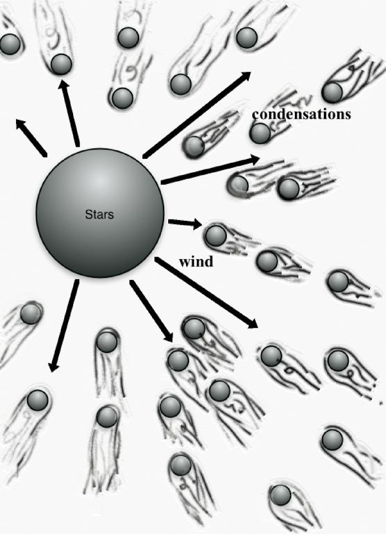
Figure 1: The drawing describing the geometry of the supercluster hot wind within which photoionized condensations are distributed.

In the broader context of the interstellar and the intracluster medium, Begelman & Fabian (1990) derived a prescription for evaluating the temperature of a turbulent mixing layer, which Slavin et al. (1993) used to calculate the emission line spectrum of such a layer. Rand (1998) established an interesting comparison between their model predictions and the spectrum produced by the diffuse gas observed in the spiral NGC 891. The models that best reproduce the observations required a mixture of TMLs and matter-bounded photoionized condensations. More recently, Binette et al. (2008; hereafter Paper I) improved earlier models in two ways: a) the hot mixing layer and the warm photoionized gas are integrated into a single albeit stratified component exposed to an external ionizing source, and b) rather than considering a single temperature for the TML given by the geometrical mean of the warm and hot phases, a temperature structure is derived using the mixing length scheme presented in the work of Cantó & Raga (1991). The possibility of computing not only emission line intensities (Binette et al. 1999), but also line profiles, has now been implemented to allow a comparison of TMLs with the very broad but faint [O iii] and H$\alpha$ wings observed in NGC 2363.

3.1 A mixing length approach

We postulate that both the narrow and the wide emission line components of the observed profiles arise from ionized gas condensations of low volume filling factor that are moving randomly. In a typical extragalactic H ii region with an H$\beta$ luminosity of $10^{40}$${\rm erg\,s^{-1}}$, this virial turbulence would give rise to a velocity dispersion of $\sim 25\,\hbox{${\rm km\,s^{-1}}$}$ (Melnick et al. 2000). In NGC 2363, we postulate the existence of a fast hot wind originating from the ionizing cluster, which flows around these condensations, giving rise to a mixing layer at their surface, as depicted in Fig. 1. It is this interaction between the fast wind and the condensations that would give rise to the observed broad component. To describe the mixing layer, we assume for simplicity an infinite plane interface, along which a hot wind of temperature $T_{w}$ is flowing supersonically with velocity $V_{w}$ with respect to a static warm gas layer of hydrogen number density $n_{o}$ and temperature $T_{o}$. The turbulent mixing layer that develops between the hot and warm phases has a geometrical thickness $l_{o}$, as described in the diagram of Fig. 2. The TML structure, the static photoionized gas and the hot wind are all isobaric, with a pressure $P_{o}$ ($\approx 2k\,\hbox{$n_{o}$}\hbox{$T_{o}$}$). The nebular optical emission lines take their origin within the warm section of the mixing layer as well as within the static photoionized layers.

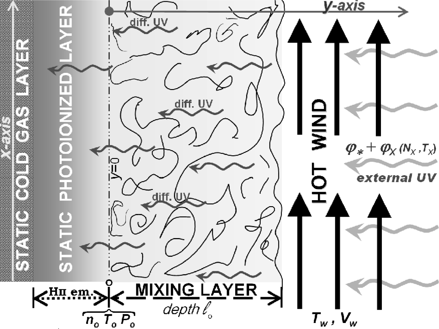
Figure 2: Schematic diagram showing the cross-section along the y-axis of a plane-parallel mixing layer of thickness $l_{o}$. The mixing layer is formed by the interaction of a supersonic wind (velocity $V_{w}$ and temperature $T_{w}$) with a static layer of warm gas of H number density $n_{o}$ and temperature $T_{o}$ (at $y=0$).

Within the TML layer, between $y=0$ and $y=\hbox{$l_{o}$}$, the gas is entrained and accelerated. From the theoretical point of view, the problem of entrainment in a mixing layer involves the description of a turbulent flow. However, following the work of Hartquist et al. (1986), Cantó & Raga (1991) developed an approximate treatment of this problem based on a mixing length approach of ‘turbulent viscosity’ and on laboratory measurements. Cantó & Raga (1991) proposed a ”single parcel” model, considering mean values for the flow variables (density, temperature, velocity) averaged across the width of the mixing layer. Noriega-Crespo et al. (1996) proposed an alternative approach, developing a model which resolves the cross section of the mixing layer (in this model, the variables correspond to averages along the $x$-axis, aligned with the direction of the shear flow). This latter approach was explored further by Binette et al. (1999). The adoption of such ‘mean’ flow characteristics allows us to get around having to deal with the details of the turbulence cascade.

For the case of a thin, steady state, high Mach number radiative mixing layer, the advective terms along the direction of the mean flow can be neglected with respect to the corresponding terms across the thickness of the mixing layer (Noriega-Crespo et al. 1996, Binette et al. 1999). Under this approximation, the momentum and energy equations can be written as:

$$\mu{d^{2}v\over dy^{2}}=0\;,$$ (1)

$$\kappa{d^{2}T\over dy^{2}}+\mu\left({dv\over dy}\right)^{2}=L-G\;,$$ (2)

where $y$ is a coordinate measured from the onset of the mixing layer (see Fig. 2), $v$ the bulk flow velocity (the velocity component projected along the $x$ axis) as a function of $y$ , $L$ and $G$ are the radiative energy loss and gain per unit volume, respectively, and $\mu$ and $\kappa$ are the turbulent viscosity and conductivity, respectively, which are assumed to be constant throughout the cross-section of the mixing layer. Eqn. 1 can be integrated to obtain the linear Couette flow solution:

$$v(y)={y\over\hbox{$l_{o}$}}\,\hbox{$V_{w}$}\;,$$ (3)

where $l_{o}$ is the thickness of the TML and $V_{w}$ is the velocity of the hot wind, parallel to the static layer. As the gas enters the TML and starts flowing, its ‘mean’ velocity in the $x$ direction increases linearly until it reaches the wind velocity at $y=\hbox{$l_{o}$}$. This solution can be substituted in Eqn. 2, which can then be integrated to derive the temperature behavior across the layer.

Within the TML, we consider the equations governing the fractional abundance $f_{i}$ of each species $i$. This abundance must satisfy the equation:

$$D{d^{2}f_{i}\over dy^{2}}=S_{f}^{i}\;,$$ (4)

where $S_{f}^{i}$ is the net sink term (including collisional ionization, radiative and dielectronic recombination, charge transfer, etc., and the reverse processes which populate the current species) of the species $i$. The turbulent diffusivity, $D$, is of order unity and assumed to be position-independent. At the inner and outer boundaries of the mixing layer, the ionization fractions are set by the equilibrium values.

To complete the description of the mixing layer, we require lateral pressure equilibrium (which determines the density of the flow along $y$), and calculate the turbulent viscosity with a simple, mixing length parametrization of the form:

$$\mu=\alpha\,{\hbox{$\overline{\rho}$}}\,\hbox{$\overline{s}$}\,\hbox{$l_{o}$}\;,$$ (5)

where $\overline{\rho}$ and $\overline{s}$ are the mass density (${\rm g\,cm^{-3}}$) and sound speed (respectively) averaged over the cross-section $l_{o}$ of the mixing layer (Fig. 2). From the work of Cantó & Raga (1991), the value of the proportionality constant $\alpha$ is $0.00247$, as described in Appendix A of Paper I. It is the required value for a supersonic mixing layer model to match the opening angle of $\approx 11^{\circ}$ of subsonic, high Reynolds number laboratory mixing layers in the limit in which the jet Mach number tends to one.

Considering that the turbulent conduction and diffusion Prandtl numbers are of order one, we can compute the conduction coefficient as $\kappa\approx\mu c_{p}$ (where $c_{p}$ is the heat capacity per unit mass averaged across the mixing layer cross-section) and the diffusion coefficient as $D\approx\mu/\hbox{$\overline{\rho}$}$. In this way, we obtain a closed set of second order differential equations (2 and 4), which can be integrated with a simple, successive overrelaxation numerical scheme.

3.2 TML calculations with the multipurpose code mappings ic

We use the code mappings ic (Ferruit et al. 1997) to compute the radiative energy loss term $L$ and the photoheating term $G$ (Eqn. 2) at each position across the TML. At both the inner and outer boundaries of the mixing layer, we assume equilibrium ionization of the different species, while across the layer, our simple overrelaxation scheme is used to determine the ionization fractions (Eqn. 4). For the ion diffusion of each species $f_{i}$, the spatial differential equations are converted to temporal equations, with the use of pseudo-time steps $\Delta t=\Delta{y}^{2}\leavevmode\nobreak\ \hbox{$l_{o}$}/(\alpha\,{\bar{n}}\,\hbox{$\overline{s}$})$, where ${\bar{n}}$ is the average H number density. This allows us to use the temporal algorithm previously described in Binette & Robinson (1987) for determining the spatial diffusion of the ionic species.

The radiative transfer is determined by integrating (from the hot layer $y=\hbox{$l_{o}$}$ down to $y=0$) the intensity of the UV diffuse field produced by the layer, assuming the outward only approximation. Any UV radiation impinging the layer from the outer boundary is simply added to the diffuse field at the onset of the integration. The intensity of the external ionizing field is defined by the ionization parameter as follows:

$$\hbox{$U_{o}$}=\hbox{$\varphi_{w}$}/c\,\hbox{$n_{o}$}\;,$$ (6)

where $c$ is the speed of light, $\varphi_{w}$ the flux of ionizing photons impinging on the TML, and $n_{o}$, the H density at $y=0$. The flux $\varphi_{w}$ is the sum of two components: $\varphi_{\ast}$ resulting from external UV sources such as hot stars and $\varphi_{X}$ due to the X-ray diffuse field generated by the hot wind (of column $N_{X}$ and average temperature $T_{X}$). In circumstances where the hot wind occupies a large volume, the soft X-ray luminosity of the hot wind can become significant despite its density, which is much lower than the optical line emitting gas. In this paper, we neglected the term $\varphi_{X}$ because the hard radiation appears to play a negligible role in comparison with the UV from the hot stars. In fact, using the diagnostic line ratio diagrams of Veilleux & Osterbrock (1987), we find that NGC 2363 occupies the same locus as that of H ii-region like galaxies (DUCBR, Gonzalez-Delgado et al. 1994).

The impact of photoionization can be inferred from the behavior of $\Gamma$ across the layer, where $\Gamma$ is defined as follows:

$$\hbox{$\Gamma$}={{L-G}\over{L+G}}\;.$$ (7)

The quantity $\Gamma$ is zero when the temperature corresponds to the equilibrium value and it is unity when cooling dominates. In our calculations, we iteratively determine $T_{o}$ at $y=0$ until the condition $\hbox{$\Gamma$}=0$ is satisfied.

For the calculations presented in this work, the mixing layers occur at the outer surface of gas condensations immersed in the radiation field of hot stars permeating supercluster A of NGC 2363. The spectral energy distribution (sed) that we adopted for $\varphi_{\ast}$ was calculated using the code LavalSB (Dionne & Robert 2006). It corresponds to a newly formed star cluster 1 Myr old, in agreement with the upper age limit derived by Drissen et al. (2000). The stellar masses are represented by a Salpeter distribution with an upper mass cut-off of 100 ${\rm M_{\sun}}$. The abundances of the atomic elements of the gas are set at 20% solar, in line with the conclusions reached by Luridiana et al. (1999).

After computing the emission line spectrum of a given TML, mappings ic offers the option of computing separately the emission lines generated by the inner photoionized layer (i.e. $y<0$ in Fig. 2) where equilibrium ionization prevails. A simple isobaric photoionization model is calculated in this case using the radiation field that has not been absorbed by the mixing layer. The total line spectrum is then given by taking the sum of the line intensities from the TML model (the broad profile component) and from the static photoionization model (the narrow profile component).

Since the mixing layer is isobaric,its density profile as a function of thickness is uniquely determined by the pressure $P_{o}$. Given the value of $n_{o}$ at the boundary $y=0$, the pressure is derived from $T_{o}$, which is the equilibrium temperature in the photoionized case. Within our selected $1.2\arcsec\times 1.2\arcsec$ aperture (Sect. 4.1), the observed [S ii] (6716/6731) ratio is 1.36, which translates into a density of 89 ${\rm cm^{-3}}$, assuming a temperature of 12 000 ^∘K. Within a factor of two, this density is also representative of the layers that emit [N ii] or [O ii]. Thus all models presented in this work were calculated assuming $n_{o}$=100 ${\rm cm^{-3}}$. It is much lower than the critical density of most atomic transitions typical of TMLs, which means that the gas density per se is not a significant parameter in these calculations. In this case, equal external parameters can be considered equivalent whenever the product of the H density $n_{o}$ and thickness $l_{o}$ is the same. Therefore, it is sufficient to specify the quantity $\hbox{$N_{\rm o}$}=\hbox{$n_{o}$}\hbox{$l_{o}$}$ to uniquely define a model, when $U_{o}$ is kept constant.

To summarize, in order to compute solutions to the mixing layer, we must specify the values of the following parameters: the ionization parameter, the mixing layer’s nominal column $N_{\rm o}$ and finally the temperature and velocity of the hot wind: $T_{w}$ and $V_{w}$.

3.3 A high-velocity hot stellar wind

The full-width at zero intensity (fwzi) of the H$\alpha$ and [O iii] profiles reaches the remarkable value of 7000 ${\rm km\,s^{-1}}$ in NGC 2363. This means that for a geometry in which the emitting gas moves radially in 3D, the velocity must extend at least up to 3500 ${\rm km\,s^{-1}}$. In practice, faster winds are required in our models, because the layers that have velocities approaching that of the wind do not produce any optical lines. The main reason is that these layers are very hot and their densities so low that their line emissivities become negligible. Another reason is that these gas layers are overionized. Towards the static layers, the temperature is close to being isothermal because photoheating equals radiative cooling. The transition between the isothermal layers and the wind dominated layers is quite abrupt. Therefore the thermal structure of TMLs consists of two zones: the isothermal warm zone and the hot thermal bump. Examples of such a thermal structure is illustrated in Fig. 3a as a function of the normalized thickness $y/\hbox{$l_{o}$}$. The three models shown are described in detail in Sect. 3.4 below and differ only by their value of $N_{\rm o}$ (hereafter $N_{\rm 20}^{\rm o}$, in units of $10^{20}$ ${\rm cm^{-2}}$). The normalized thickness maps directly into the velocity domain, since the Couette flow solution implies a linear velocity increase between the static layer and the wind flow (Eqn. 3). If we define $\epsilon$ as the fraction of the layers’ thickness where $T_{w}$ is isothermal, which turns out to be where the optical lines are produced, it follows that a wind velocity of $3500\,\hbox{$\epsilon$}^{-1}$ ${\rm km\,s^{-1}}$ is required to cover the velocity span observed in NGC 2363. We could not get credible calculations that had $\hbox{$\epsilon$}\geq 0.9$. The model with $\hbox{$N_{\rm o}$}=33$ in Fig. 3a has $\hbox{$\epsilon$}=0.81$. Hence, in order to reproduce the observed broad wings, it is necessary to adopt a wind velocity as high as $\hbox{$V_{w}$}\simeq 4300$ ${\rm km\,s^{-1}}$. This value is somewhat higher than the 3500 ${\rm km\,s^{-1}}$ value calculated by Sternberg et al. (2003) for O3 stars.

Rather than a single stellar wind, we propose that we have a wind from a dense cluster of massive stars. As shown by Cantó et al. (2000), the resulting cluster wind has a terminal velocity equal to the velocity of the winds from the cluster stars. Also, the interaction of the different winds results in a very high initial temperature for the cluster wind ($\sim 10^{8}\,{}^{\circ}$K for the wind velocity we are proposing), but this temperature rapidly drops beyond the outer radius of the cluster, as the cluster wind approaches its terminal velocity.

Another alternative to a stellar origin for the wind is that it has been generated by supernovae. There is, however, no evidence of past supernovae in knot A although we cannot entirely rule it out. In knot B, there is evidence of a cavity surrounding the central stellar cluster, which might have been caused by supernovae explosions. The explanation provided by Drissen et al. (2000, 2001) is that supercluster A is extremely young ($\la 1$ Myr) while supercluster B is older ($\sim 3$–4 Myr).

We found that the temperature $T_{w}$ of the hot wind is not a critical parameter of the TML models. Its value can be varied and still result in a sequence of equivalent models (i.e. with similar line ratios), provided $V_{w}$ remains the same. However, to ensure that the X-ray flux from the hot wind would not be excessive, we have set its temperature to $\hbox{$T_{w}$}=5\times 10^{5}\,{}^{\circ}$K in all our calculations. The non-detection of NGC 2363 by the satellite XMM-Newton in the 0.1–10 keV X-ray band has allowed the determination of an upper limit of $4\times 10^{-13}$ ${\rm erg}\,{\rm cm}^{-2}\,{\rm s}^{-1}$ (Y. Krongold & E. Jimenez-Bailon, private communication). Using the code MEKAL (Mewe et al. 1986; Liedahl et al. 1995) and assuming a cylinder of hot gas of radius 10 pc, length 100 pc and density $\hbox{$n_{w}$}=100\,\hbox{${\rm cm^{-3}}$}\times 12\,000\,^{\circ}{\rm K}/\hbox{$T_{w}$}=2.4\,\hbox{${\rm cm^{-3}}$}$, one of us (Y. K.) recently determined that the wind would emit a flux more than an order of magnitude lower than the above upper limit. Thus, even much higher wind temperatures ($\sim 10^{8}\,{}^{\circ}$K) would neither produce a flux that exceeded this upper limit.

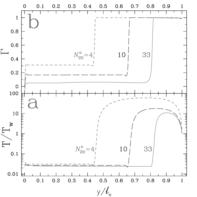
Figure 3: Behavior in panel a of the temperature normalized to the value in the wind and in panel b of $\Gamma$ (Eqn. 7), both as a function of the normalized thickness $y/\hbox{$l_{o}$}$. The three models shown vary only by their mixing layer nominal column: $\hbox{$N_{\rm 20}^{\rm o}$}=4$, 10 and 33.

3.4 Internal structure of three test models

After defining the stellar sed, density and wind characteristics, we can now proceed with the calculations. In order that the line ratios of the photoionized layers could match the nebular values, we selected a high ionization parameter $\hbox{$U_{o}$}=0.02$. The total [O iii]/H$\beta$ ratio, including the static gas emission, is $\approx 8.1$, which is comparable to the observed ratio of 8.9. Our main aim is to reproduce the broad lines profiles and therefore no further analysis of the line ratios of the cores of the profiles has been attempted. In Fig. 3, apart from $T_{w}$, we also show the behavior of the measured imbalance between cooling and heating, $\Gamma$ (see Eqn. 7), as a function of normalized thickness for each of the three models whose mixing layer’s column differ and take on values of $\hbox{$N_{\rm 20}^{\rm o}$}=4$, 10 and 33, in units of $10^{20}$ ${\rm cm^{-2}}$. For each model, the ionization parameter is $\hbox{$U_{o}$}=0.02$ and the wind temperature and velocity are $\hbox{$T_{w}$}=5\times 10^{5}\,{}^{\circ}$K and $\hbox{$V_{w}$}=4300$ ${\rm km\,s^{-1}}$, respectively. The equilibrium temperatures at the onset of the layer are $\hbox{$T_{o}$}=11\,460$, 11 330 and 12 370 ^∘K for the models with $\hbox{$N_{\rm 20}^{\rm o}$}=4$, 10 and 33, respectively. Because $\epsilon$ increases with $N_{\rm 20}^{\rm o}$, these TML models result in a broad profile whose width increases monotonically with $N_{\rm 20}^{\rm o}$. Alternatively, a sequence of increasing profile’s width can be obtained by increasing $V_{w}$ while keeping $N_{\rm 20}^{\rm o}$ constant.

It is well known that the cooling rate $L$ of a hot plasma decreases with temperature when its value lies above $\approx 2\times 10^{5}\,{}^{\circ}$K (e.g. Fig. 8 in Ferruit et al. 1997). This behavior of the cooling is responsible for the temperature bump towards the interface with the wind, which is apparent in Fig. 3. In effect, near the wind interface, the heating from turbulent dissipation overwhelms radiative cooling and results in $\Gamma$ near unity. It also results in an overionized plasma of very low density (hence low emissivity), which does not generate significant line emission, at least in the optical domain. The impact of heating by turbulent dissipation increases considerably when we consider thinner mixing layers, as can be seen in Fig. 3. Towards the colder gas layers, radiative cooling becomes sufficiently strong to enable a balance between radiative cooling and heating by photoionization and turbulent dissipation. Although heating by photoionization dominates in the near-isothermal region, turbulent dissipation is nevertheless present as indicated by $\Gamma$, which reaches 0.3 in the case of the $\hbox{$N_{\rm 20}^{\rm o}$}=4$ model.

3.5 Projection in 3D and line profile calculations

In order to derive the integrated line profiles from the 3D distributions of gas condensations, we first compute the profile from a single condensation at the surface of which the fast wind generates a TML. We neglect the details of the contours of such condensation and consider that the TML takes place on the sides of the condensation, as if it was a cylinder whose axis is oriented radially with respect to the wind source. In Fig. 4 we show the resulting emission flux from the same three models of Sect. 3.4, as a function of radial velocity. The vertical scale is arbitrary between models, but remains the same for lines of the same model. These 1D profiles correspond to a single condensation that lies exactly along our line-of-sight to the wind source. The profiles have been initially smoothed in mappings ic by a narrow gaussian of 25 ${\rm km\,s^{-1}}$ dispersion (see Sect. 3.1), which accounts for the virial broadening due to the supersonic motions of the condensations. To a first order and for most optical lines, the profiles resemble a top-hat function that extends up to a limit, $V_{lim}$. The velocity limits up to which the H$\alpha$ or [O iii] flux extends are $\hbox{$V_{lim}$}=-1900$, $-$2800 and $-$3440 ${\rm km\,s^{-1}}$ for the models with $\hbox{$N_{\rm 20}^{\rm o}$}=4$, 10 and 33, respectively. This top-hat shape is the result of the Couette flow solution, which corresponds to a velocity that increases linearly with $y$ (Eqn. 3). The He ii line is an exception because it is mainly produced at the onset of the thermal bump. $V_{lim}$ is lower than $V_{w}$ since the optical line emissivities become negligible inside the overionized thermal bump region, as discussed above. Essentially, all of the flux originates from the near-isothermal region (depicted in Fig. 3). The thinner the TMLs gets, the smaller becomes the region where emission takes place, which results in proportionally narrower line profiles. Furthermore, the model with $N_{\rm o}$=33 is ionization-bounded, while the other two with $N_{\rm o}$=10 and 4 are matter-bounded, which result in significantly higher [O iii]/H$\beta$ line ratios, of 10.8 and 15.7, respectively.

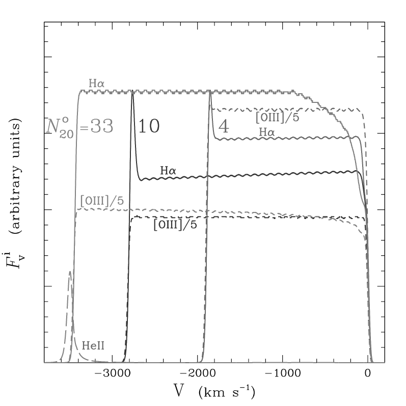
Figure 4: Emission line flux from H$\alpha$ (solid line) and [O iii]$\lambda$5007 (dashed line) as a function of radial velocity is plotted for each of the three models of Fig. 3. Note that the [O iii] fluxes have been scaled down by a factor 5. The He ii $\lambda$4686 emission flux is shown in the case of the $N_{\rm 20}^{\rm o}$=33 model only.

The emission profiles of Fig. 4 apply to the simple one-dimension case. We will now consider the more realistic case of a radial wind in 3D and compute the profile that would be seen by a distant observer. To achieve this, we assume some simplifications about the problem, namely, that all the TMLs are immersed in a radial constant velocity wind, the wind is isotropic with respect to the wind source and the covering factor $C_{f}$ of the mixing layers is also isotropic. To simplify things further, we will assume that the TMLs are located at the same radius $R$ from the central source of the wind. For any emission line $i$ at rest-wavelength $\lambda_{o}^{i}$, these considerations lead to the following integral for the flux:

$$\begin{array}[]{rlllll}F_{v}^{i}&=2\pi R^{2}C_{f}\left\{{\int_{\hbox{$\theta_{i}$}}^{\hbox{$\theta_{f}$}}}F^{i}\!(v^{\prime})\sin\theta d\theta\right.\\ +&\left.{\int_{\frac{\pi}{2}+\hbox{$\theta_{i}$}}^{\frac{\pi}{2}+\hbox{$\theta_{f}$}}}F^{i}\!(-v^{\prime})\,\exp\!\left(-\tau_{\lambda_{o}^{i}}\cos\theta\right)\sin\theta d\theta\right\},\\ F^{i}\!(v^{\prime})&=\sec\theta\,F^{i}\!(v\cos\theta)\;,\\ v^{\prime}&=v\cos\theta\;,\\ \tau_{\lambda_{o}^{i}}&=\sigma_{d}^{i}\,n_{\!d}\,2R\;,\\ v&=c(\lambda-\lambda_{o}^{i})/\lambda_{o}^{i}\;,\end{array}$$ (14)

where $c$ is the speed of light, $\theta$ the angle with respect to the line-of-sight to the observer, $R$ the radius where the TMLs are located with respect to the wind source, and $F^{i}\!(v)$ in the integrand is the emission flux for line $i$ as computed by mappings ic (i.e. for $\theta=0$). To include the possibility that dust might fill the volume of the sphere of radius $R$ and thereby absorb line emission from the (red-shifted) TMLs on the far-side, we introduce in Eqn. 14 a dust extinction cross-section $\sigma_{d}^{i}$ evaluated at $\lambda_{o}^{i}$. The parameter $n_{\!d}$ is the dust grain density filling the sphere and $\tau_{\lambda_{o}^{i}}$ is the resulting line extinction due to dust. The effect of internal dust would be to skew the profile towards the blue. Since we found no evidence of profile asymmetry, we have set $n_{\!d}=0$. There could be additional ‘intervening’ dust that covers the whole nebula, however. This possibility is not relevant to our profile study since the differential reddening across the profile width turns out to be negligible, assuming a $C({\rm H}\beta$) of 0.2 for knot A (Gonzalez-Delgado et al. 1994). As for the two limits of integration, whenever the TML system (of projected area $\pi{R}^{2}$ on the sky) is fully contained within the aperture of the spectrograph, these reduce to $\hbox{$\theta_{i}$}=0$ and $\hbox{$\theta_{f}$}=\pi/2$, which is what is assumed hereafter. We have explored relaxing this assumption. With $\hbox{$\theta_{f}$}\la\pi/2$, the profiles become flat-topped while for $\hbox{$\theta_{i}$}\ga{0}$, the profiles does not change much in shape but becomes progressively narrower. In a more realistic description, the TMLs would cover a range in radii and $C_{f}$ would be a function of radius. The current description, however, suffices to capture the basic implication of a 3D geometry on the line profiles.

4 Comparison of TML profiles with the observations

4.1 Characteristics of the broad profile wings

We analyzed a subset of the available data as follows. To derive the highest S/N possible, we considered a square region of $1.2\arcsec\times 1.2\arcsec$ ($20\times 20$ pc) centered on knot A and extracted a red and a blue spatially-collapsed spectra within this area. We modeled the underlying continuum and subtracted it from both the H$\alpha$ and [O iii]$\lambda$5007 lines. In order to facilitate the comparison of the models with the faint broad wings observed in [O iii] and H$\alpha$, we converted the profiles into velocity space relative to the centroid of each line. Direct profile comparison is achieved by simply superposing different lines.

At the time of writing, various issues concerning the absolute calibration of the blue spectrum could not be satisfactorily resolved. In what follows, we will not rely on the absolute flux scale of the blue spectrum, but focus instead on profile shape comparisons or on relative ratios of the broad component with respect to the central core component. After rescaling the blue spectrum until the broad [O iii] superimposes the broad H$\alpha$ profile, one finds that the ‘shape’ of the broad component is the same in both lines. This is apparent in Fig. 5, where the H$\alpha$ profile as a function of Doppler velocity is shown in red and [O iii]$\lambda$5007 in blue. To express fluxes, the quantity $\hbox{$F^{v}_{\rm 15}$}=10^{15}F_{v}$ is used hereafter. The H$\alpha$ line peaks at a value of $F^{v}_{\rm 15}$=853 (but not [O iii]  which has been rescaled in this figure). No reddening correction has been applied. We now discuss plausible interpretations of the scaling factors that are obtained from superimposing line profiles.

Detailed analysis showed that if we scaled the [O iii] line profile so that the peak of its narrow core equalled that of H$\alpha$, the broad wings of H$\alpha$ were brighter than [O iii] by about 50%. If instead of [O iii], we overlaid the continuum subtracted H$\beta$ line and rescaled it so that the peak of its narrow core equalled that of H$\alpha$, we similarly found that the broad H$\alpha$ lies $\approx 50$% higher than the broad H$\beta$. We verified that saturation is not taking place. Flux spilling over nearby pixels appears also to be ruled out. A possible interpretation is that the gas responsible for the faint broad wings is further absorbed by dust than the gas responsible for the bright narrow core. Apart from our basic conclusion that the broad [O iii] and H$\alpha$ profiles are of similar shapes, which suggests that the broadening mechanism acts uniformly on both lines, we find that the data is consistent with the broad [O iii]/H$\beta$ flux ratio being the same as that of the narrow core [O iii]/H$\beta$. This follows from the two separate comparisons above that indicated that the broad H$\beta$ and [O iii] are depressed by the same factor with respect to the broad H$\alpha$. It is noteworthy that these two conclusions are not affected by our calibration uncertainties.

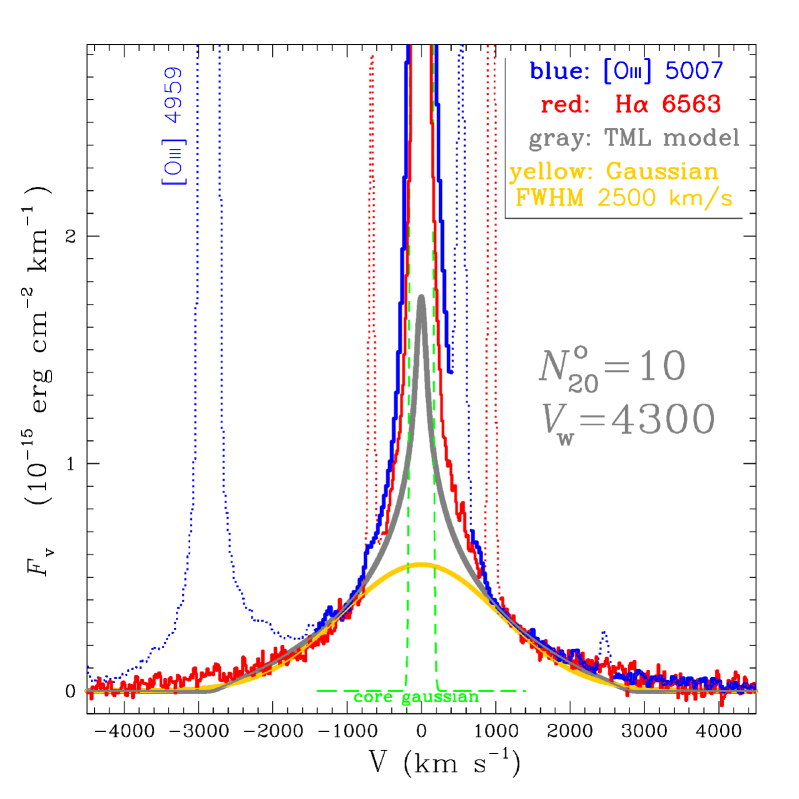
Figure 5: Superposition of the emission line profiles of H$\alpha$ (red line) and of [O iii]$\lambda$5007 (blue line) as a function of Doppler velocity with respect to the centroid of both lines. The scale applies to H$\alpha$ and the units are ${\rm erg}\,{\rm cm}^{-2}\,{\rm km}^{-1}$. The [O iii] profile has been scaled up so that its broad wings coincided as much as possible with those of H$\alpha$. Emission lines involving other energy levels have been partially blanketed with dotted line contours. Using a thick gray line, we overlaid the 3D profile from a TML model with $N_{\rm 20}^{\rm o}$=10 and $V_{w}$=4300 ${\rm km\,s^{-1}}$. The yellow line shows how a broad Gaussian of 2500 ${\rm km\,s^{-1}}$ fwhm would compare. The green colored dashed-line is a fwhm=110 ${\rm km\,s^{-1}}$ Gaussian fit of the narrow core component.

Hereafter we will concentrate on the faint broad profiles shown in Fig. 5. As discussed above, the [O iii], H$\alpha$ and H$\beta$ broad profiles are characterized by a similar functional dependence on velocity. This similarity in shape and the fact that the integrated [O iii]/H$\beta$ flux ratio for the wings is the same as for the narrow core imply stringent constraint for any proposed model. It suggests that the physical conditions pertaining to the gas that produces the faint broad wings are very likely similar to those of the more quiescent nebular gas.

The fwhm of the core of the profiles was derived by fitting a single Gaussian. We obtained 78 and 115 ${\rm km\,s^{-1}}$ for H$\alpha$ and [O iii], respectively. The [O iii] core profile is unresolved and appears broader due to the lower resolution of the blue grating. In order to distinguish at which velocity the broad line flux exceeds the intense flux from the narrow core, we overlay in Fig. 5  a Gaussian fit (green dashed line) to the narrow core (with fwhm=110 ${\rm km\,s^{-1}}$). We infer that the observed profiles becomes noticeably wider than the narrow Gaussian below $\hbox{$F^{v}_{\rm 15}$}\approx 2$, which lies at only 0.23% of the peak flux value. Note that the width of the narrow Gaussian is 325 ${\rm km\,s^{-1}}$ at $F^{v}_{\rm 15}$=2.

4.2 Comparison with 3D TML line profiles

Since our main aim is to reproduce the weak broad wings underneath each line, we now focus on the profiles generated by the TML, leaving out the narrow line component produced by the static layer at the surface of the condensations. Since the emission flux from the broad component is proportional to the surface area of the TML gas exposed to the ionizing radiation, this area has to be quite small ($\approx 3$%) relative to that of the nebular gas (the ‘static’ or narrow line component).

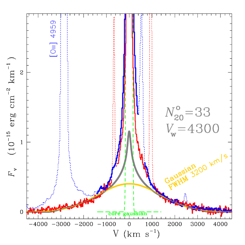
Figure 6: Same notation as in Fig. 5 except for the TML model, which corresponds to $N_{\rm 20}^{\rm o}$=33. For comparison, a Gaussian of 3200 ${\rm km\,s^{-1}}$ fwhm is overlayed.

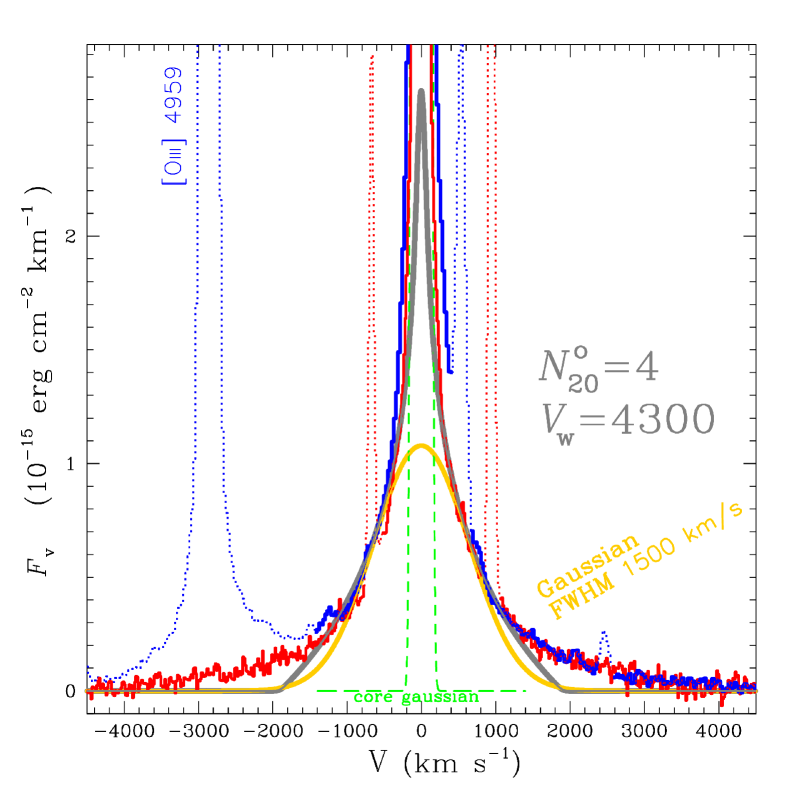
Figure 7: Same notation as in Fig. 5 except for the TML model, which corresponds to $N_{\rm 20}^{\rm o}$=4. For comparison, a Gaussian of 1500 ${\rm km\,s^{-1}}$ fwhm is overlayed.

We applied the profile integral described in Eqn. 14, which considers the effects of velocity projection in 3D, to each of the three TML models shown in Fig. 4. Because the narrow line cores in NGC 2363 have a width that exceed the value assumed by mappings ic (25 ${\rm km\,s^{-1}}$, see Sec. 3.1), we further convolved the calculated profiles using a narrow Gaussian of 107 ${\rm km\,s^{-1}}$ fwhm. The fwhm describing the velocity dispersion of the condensations (Fig. 1) also applies to the TMLs.

The TML model of the [O iii] line assuming $\hbox{$N_{\rm 20}^{\rm o}$}=10$ is superimposed to the data in Fig. 5 (gray line). It is unnecessary to superimpose the H$\alpha$ model separately, since it is visually undistinguishable from the [O iii] model, even if the difference in spectral resolution were considered in the modeling. The profile fit that is achieved of the broad wings, although clearly imperfect, is certainly encouraging, given the approximations made to the transfer and to the geometry of the TMLs. Because Gaussians are a natural profile for describing emission lines over a wide variety of physical situations, we also compared our data with simple Gaussian profiles. In Fig. 5, the yellow line represents a Gaussian with an fwhm of 2500 ${\rm km\,s^{-1}}$. We find that our TML model provides a better description of the data. (Gaussians with different fwhm are drawn in the subsequent Figures 6 and 7). There is definitely more flux present at both low and high velocities in the observed profiles than provided by any single broad ‘Gaussian’. The same appears to be the case for the TML model with $N_{\rm o}$=10, but to a much lesser extent. For instance, the TML profile fills the widening of the profile beyond the narrow Gaussian core (dashed green line) much better compared to the round top of a wide Gaussian. A Lorentzian profile would provide a better description of the data than a Gaussian, as shown in Fig. 8. However, given the physical characteristics of the gas, there is no physical justification for a Lorentzian profile.

In Figs. 6 and 7, we show the other two TML models of equal $V_{w}$, but with different $N_{\rm 20}^{\rm o}$ of 33 and 4, respectively. The model that fits the wings better (Fig. 6) does worse with the core region, and conversely with the other model. For comparison, Gaussians that approximately match the same region as the corresponding TML model are overlaid.

To obtain a much improved fit to the profile wings, the juxtaposition of two or more TML profiles of different widths would therefore be necessary. Because the [O iii]/H$\beta$ ratio varies markedly along the $N_{\rm o}$ sequence (Sect. 3.5) and since the observed broad [O iii]/H$\beta$ line ratio is the same as the one found for the narrow core, we would argue against combining models of different thickness $N_{\rm o}$. An alternative way to combine TML profiles would be to consider a radial gradient in wind velocity $V_{w}$. Such a sequence in which $V_{w}$ varied and $N_{\rm o}$ remained at the value set by the ionization-bounded case would present a clear advantage, since the resulting [O iii]/H$\beta$ ratio would not change from the value characterizing the static nebula case.

To illustrate this, we looked for an ionization-bounded model that would be equivalent to the model with $N_{\rm 20}^{\rm o}$=10 (Fig. 5, which is the model that fits relatively well the bulk of the broad profile). In this new model, the increase in thickness is compensated by a reduction in wind velocity. The resulting profile is shown in Fig. 8 and corresponds to a slower wind of $V_{w}$=3500 ${\rm km\,s^{-1}}$ and a larger thickness $N_{\rm 20}^{\rm o}$=31. The comparison of Fig. 8 with Fig. 5 shows that the two profiles are comparable. In the case of the slower wind model, the broad profile is slightly wider because $\epsilon$ is larger (0.88) and it fares better in the wings than the 4300 ${\rm km\,s^{-1}}$ model with $N_{\rm 20}^{\rm o}$=10. This new model is preferable, since it results in the same [O iii]/H$\beta$ ratio as that of the narrow core. Furthermore, the wind velocity is more conservative and corresponds to the value calculated by Sternberg et al. (2003) for O3 stars.

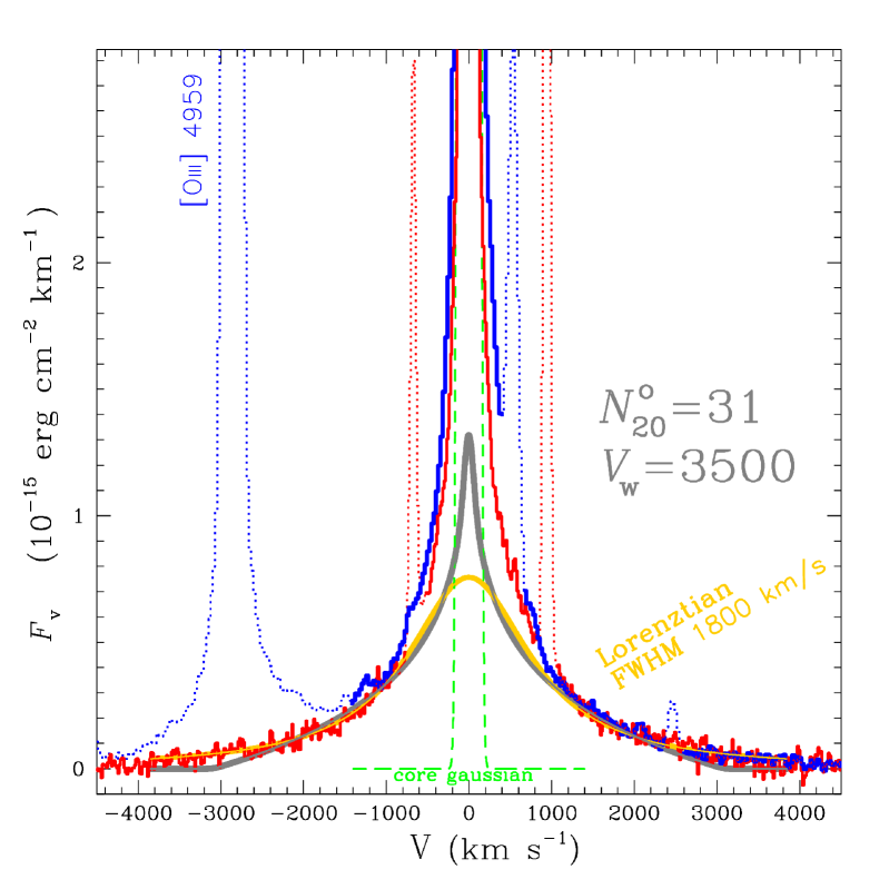
Figure 8: Same notation as in Fig. 5 except for the TML model, which corresponds to a slower wind of $V_{w}$=3500 ${\rm km\,s^{-1}}$ with $N_{\rm 20}^{\rm o}$=31. For comparison, a Lorentzian profile of 1800 ${\rm km\,s^{-1}}$ fwhm is overlayed.

4.3 Other emission lines

The TML models predict that there should not be any broad wings underneath the lower excitation lines such as [N ii] or [S ii]. The reason is that in models with a high ionization parameter (e.g. $\hbox{$U_{o}$}\ga 0.01$) the degree of ionization throughout the turbulent layer is high and the ionized gas is dominated by high excitation species, such as O⁺² or N⁺². This means that low excitation species are relatively insignificant throughout the layer. Inspection of the data shows no evidence of broad wings underneath the low excitation lines at a level comparable to that observed in H$\alpha$, H$\beta$ or [O iii]. We have also explored whether faint wings would be present underneath the high excitation lines, as is predicted by the model. The limited S/N available for the weak [Ar iv] lines, however, has made such a test inconclusive.

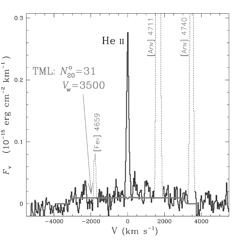
Figure 9: Observed emission line profiles of He ii $\lambda$4686 (black line) as a function of Doppler velocity with respect to the centroid of both lines. Other line transitions near He ii have been blanketed by dotting the corresponding line. We overlay a 3D profile from a TML model (gray line) with $V_{w}$=3500 ${\rm km\,s^{-1}}$ and $N_{\rm 20}^{\rm o}$=31, but with its intensity multiplied by a factor 5.

The shapes of the profiles predicted by the TML models are either characterized by a broad profile with a peaked center ([O iii], C iv, C iii], [Ne iii], H$\alpha$, H$\beta$) or a narrow core without any significant wings ([S ii], Mg ii, [N ii], [O ii]). There are a few exceptions, however, such as the high excitation line of He ii $\lambda$4686, which presents a top hat shape. This arises as the line is only produced significantly at the onset of the thermal bump in Fig. 3 where the temperature shoots up above that of the isothermal region (see He ii emission flux in Fig. 4). For illustrative purposes we show the profile predicted for He ii in Fig. 9. It corresponds to an upper limit equivalent to 5 times the intensity predicted by the TML model with $V_{w}$=3500 ${\rm km\,s^{-1}}$ and $N_{\rm 20}^{\rm o}$=31. It is possible that mappings ic underpredicts the strength of this line, since it considers only pure recombination and does not include collisional excitation. It is interesting to note that one cannot completely rule out the presence of a weak broad component (or flat pedestal) underneath the narrow He ii profile. We do not expect such a component to be due to a Wolf-Rayet feature, since supercluster A in NGC 2363 is much too young ($<1$ Myr; Drissen et al. 2000) and, furthermore, no evidence has been found of broad N iii] or C iv, which are otherwise expected if Wolf-Rayet stars were present.

4.4 Line profiles from starburst galaxies

A different area where TML emission could play a role are broad profiles, with fwhm in the range of 150–400 ${\rm km\,s^{-1}}$, observed in starburst galaxies, such as NGC 1569 (Westmoquette et al. 2007a, b, 2008) or M82 (Westmoquette et al. 2007c). The requirements for wind velocities in these objects are modest in appearance, which implies a much lower wind velocity. However, the fwhm observed may nevertheless correspond to a significantly higher $V_{w}$ if the wind, rather than being fully isotropic, tended to project along the plane of the sky of the observer. For instance, in the case of near edge-on galaxies, the wind can be funneled above and below the galactic plane, resulting in a narrower profile because $\hbox{$\theta_{i}$}>0$, in the notation of Sect. 3.5. In contrast to NGC 2363, supernovae can play an important role in launching starburst winds. Another significant difference is that it is the lower excitation lines like [N ii]$\lambda$6583 that are observed to be broad. This can only be accounted for in our model if a sufficiently low ionization parameter is assumed, which could ensure that the intermediate excitation lines spread over a significant fraction of the TML’s thickness. A softer ionizing continuum due to high metallicities may also contribute to the prominence of intermediate excitation lines. In the case of M82, Westmoquette et al. (2007c) report a relatively low [O iii]/H$\beta$ (5007/4861) ratio of $\simeq 0.32$. New TML calculations adapted to the context of starburst galaxies would be required to verify whether the inferred ionization parameter is sufficiently low for the [N ii] lines to become broad as well.

5 Conclusions

Four mechanisms have been explored by Roy et al. (1992) to account for the extreme gas velocities observed in NGC 2363, namely stellar winds, Thomson scattering by hot electrons, supernova remnants, and a superbubble blowout. These authors reported significant problems with each of these mechanisms and considered them to be unsatisfactory. They concluded that the broad nebular gas is probably due to “very high velocity gas whose origin is, at present, unknown”. In this paper, we explore the possibility that the broad emission originates from turbulent mixing at the interface between a hot cluster wind and more quiescent photoionized condensations. In our model, all gas phases are in pressure equilibrium and, because of the high temperature of the wind, the total ionized gas mass contained in the wind is much lower than postulated by Roy et al. (1992), by a factor $\sim\hbox{$T_{w}$}/10^{4}$. Since the upper limits on $T_{w}$ set by the non-detection in the X-rays allows temperature values as high as $10^{8}\,{}^{\circ}$K (Sect. 3.3), the objection to the wind hypothesis expressed by Roy et al. can be lifted.

The basic input parameters affecting the TML models have been given appropriate values as follows: we inferred a density of $\simeq 100$ ${\rm cm^{-3}}$ for the nebular gas, using the [S ii] doublet. The metallicity that was assumed is 20% solar, as deduced by Luridiana et al. (1999). The sed that we adopted was calculated using the code LavalSB and corresponds to a newly formed star cluster 1 Myr old [the upper age limit derived by Drissen et al. (2000)]. Finally, the ionization parameter has been adjusted so that the calculated [O iii]/H$\beta$ ratio became comparable to the observed value.

In our model, the broad profile results from radial acceleration in 3D of photoionized turbulent gas. About 10–20% of the acceleration that takes place occurs at temperatures approaching that of the wind, and this gas does not contribute to line emission. For this reason, the wind velocity assumed in the TML model must exceed the value inferred from the extent of the faint wings (i.e. $\pm 3500$ ${\rm km\,s^{-1}}$). To constrain the models, we adopted the spectral data set of Drissen et al. (2009) that was obtained at the Gemini observatories. We report in Sect. 4.2 on the results of models with $\hbox{$V_{w}$}=4300$ ${\rm km\,s^{-1}}$, which can successfully fit the faint wings when the TML is ionization bounded ($N_{\rm 20}^{\rm o}$=33; Fig. 6). The bulk of the profile is better fitted if we reduced the TML thickness to $\hbox{$N_{\rm 20}^{\rm o}$}\simeq 10$ (Fig. 5). This model, however, is matter-bounded and the [O iii]/H$\beta$ ratio from the TML would exceed that observed in the core of the lines as well as in the broad component. Our preferred scenario, therefore, is that the cluster wind undergoes radial acceleration, but the TML remains ionization-bounded at all radii. Our slower wind model of 3500 ${\rm km\,s^{-1}}$ and with $N_{\rm 20}^{\rm o}$=31 is as successful in fitting the bulk of the broad profile (Fig. 8). It is therefore our best model overall. The relative success of TMLs in fitting broad profiles and in predicting the absence of broad lines for [N ii] and [S ii] are significant arguments in favor of the models. The requirement of wind velocities of order 4000 ${\rm km\,s^{-1}}$ in order to fit the very faint wings remain a stumbling block, however, unless supercluster A, because of its extreme youth, is able to generate such physical conditions. Interestingly, our TML model results in a flat-top profile for He ii $\lambda$4686, although this characteristics could not be confirmed with the current data. As a follow-up study, new calculations adapted to the broad component observed in starburst galaxies (e.g. Westmoquette et al. 2007a, b, c) should be carried out along the lines developed in Sect. 4.4.

Although, in this paper, the accelerating mechanism is assumed to arise from a stellar wind, alternative mechanisms could be considered that would lead to a near-constant radial acceleration and therefore generate profiles equivalent to those shown in this work. One possibility for instance might be radial acceleration due to radiation pressure acting on dusty photoionized gas plumes. NGC 2363 is clearly a fascinating object that remains a challenge in our understanding of extremely young nebulae.