Unconventional pairing originating from disconnected Fermi surfaces in the iron-based superconductor

Abstract

For the iron-based high $T_{c}$ superconductor LaFeAsO_1-xF_x, we construct a minimal model, where all of the five Fe $d$ bands turn out to be involved. We then investigate the origin of superconductivity with a five-band random-phase approximation by solving the Eliashberg equation. We conclude that the spin fluctuation modes arising from the nesting between the disconnected Fermi pockets realise, basically, an extended $s$-wave pairing, where the gap changes sign across the nesting vector.

,

1 Introduction

While the physics of high-$T_{c}$ cuprate has matured after the two decades since the discovery, the superconductivity the iron-based pnictide LaFeAsO doped with fluorine discovered by Hosono’s group[1] is more than welcome as a fresh challenge for yet another class of high-$T_{c}$ systems. Indeed, the iron-based material, along with various other ones in the same family of compounds with higher transition temperatures ($T_{c}$)[2], are remarkable as the first non-copper compound that has $T_{c}$’s exceeding 50 K. This immediately stimulates renewed interests in the electronic mechanism of high $T_{c}$ superconductivity. In order to investigate the pairing mechanism, here we first construct an electronic model for LaFeAsO_1-xF_x using maximally localised Wannier orbitals obtained from first principles calculation. The minimal model turns out to involve all the five Fe $d$ orbitals.[3] Hence the iron-based material is contrasted with the cuprate, which is a one-band, doped Mott insulator. We then apply the random-phase approximation (RPA) to solve the Eliashberg equation. We conclude that a nesting between multiple Fermi surface (pockets) results in a development of a peculiar spin fluctuation mode, which in turn realises an unconventional pairing, which is basically an extended $s$-wave where the gap function changes sign across the nesting vector.[3, 4] The result is intriguing as a realisation of the general idea that the way in which electron correlation effects appear is very sensitive to the underlying band structure and the shape of the Fermi surface.[5]

2 Band structure

LaFeAsO has a layered structure, where Fe atoms form a square lattice in each layer, which is sandwiched by As atoms.[6] Due to the tetrahedral coordination of As atoms, there are two Fe atoms per unit cell. The experimentally determined lattice constants are $a=4.03$Å and $c=8.74$Å, with two internal coordinates $z_{\rm La}=0.142$ and $z_{\rm As}=0.651$.[7] We have first obtained the band structure (Fig.1) for these coordinates with the density-functional approximation with plane-wave basis[8], which is then used to construct the maximally localised Wannier functions (MLWFs)[9]. These MLWFs, centered at the two Fe sites in the unit cell, have five orbital symmetries ($d_{3Z^{2}-R^{2}}$, $d_{XZ}$, $d_{YZ}$, $d_{X^{2}-Y^{2}}$, $d_{XY}$, where $X,Y,Z$ refer to those for this unit cell with two Fe sites as shown in the bottom panel of Fig.1). The two Wannier orbitals in each unit cell are equivalent in that each Fe atom has the same local arrangement of other atoms. We can then take a unit cell that contains only one orbital per symmetry by unfolding the Brillouin zone,[10] and we end up with an effective five-band model on a square lattice, where $x$ and $y$ axes are rotated by 45 degrees from $X$-$Y$. We refer all the wave vectors in the unfolded Brillouin zone hereafter. We define the band filling $n$ as the number of electrons/number of sites (e.g., $n=10$ for full filling). The doping level $x$ in LaFeAsO_1-xF_x is related to the band filling as $n=6+x$.

The five bands are heavily entangled as shown in Fig.2 (left panel) reflecting strong hybridisation of the five $3d$ orbitals, which is physically due to the tetrahedral coordination of As atoms around Fe. Hence we conclude that the minimal electronic model requires all the five bands. In Fig.2(right), the Fermi surface for $n=6.1$ (corresponding to $x=0.1$) obtained by ignoring the inter-layer hoppings is shown in the two-dimensional unfolded Brillouin zone.

The Fermi surface consists of four pieces (pockets in 2D): two concentric hole pockets (denoted here as $\alpha_{1}$, $\alpha_{2}$) centered around $(k_{x},k_{y})=(0,0)$, two electron pockets around $(\pi,0)$ $(\beta_{1})$ or $(0,\pi)$ $(\beta_{2})$, respectively. $\alpha_{i}$ ($\beta_{i}$) corresponds to the Fermi surface around the $\Gamma$Z line (MA in the original Brillouin zone) in the first-principles band calculation.[11] Besides these pieces of the Fermi surface, there is a portion of the band near $(\pi,\pi)$ that is flat and touches the $E_{F}$ at $n=6.1$, so that the portion acts as a “quasi Fermi surface $(\gamma)$” around $(\pi,\pi)$, which has in fact an important contribution to the spin susceptibility. As for the orbital character, $\alpha$ and portions of $\beta$ near Brillouin zone edge have mainly $d_{XZ}$ and $d_{YZ}$ character, while the portions of $\beta$ away from the Brillouin zone edge and $\gamma$ have mainly $d_{X^{2}-Y^{2}}$ orbital character (Fig.3, bottom panels).

An interesting feature in the band structure is the presence of Dirac cones, i.e., places where the upper and the lower bands make a conical contact. [12, 13] The ones closest to the Fermi level lies at positions where the $d_{X^{2}-Y^{2}}$ and the $d_{XZ}/d_{YZ}$ bands cross, just below the $\beta$ Fermi surface.

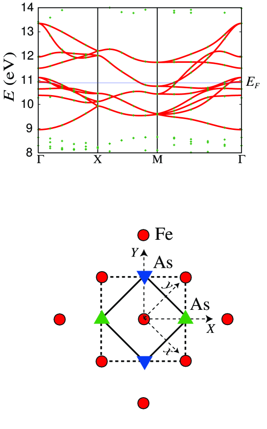
Figure 1: Top panel: The band structure of in the original (folded) Brillouin zone, where the symbols represent the LDA result while curves the ten-band model derived with the maximally localised Wannier orbitals. Bottom panel: The original (dashed) and the reduced (solid) unit cells in real space with $\bullet$ (Fe), $\nabla$ (As below the Fe plane) and $\triangle$ (above).

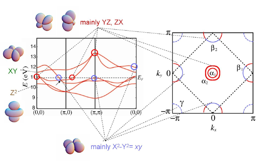
Figure 2: Left: The band structure of the five-band model in the unfolded Brillouin zone. Orbital characters of the bands are also indicated. The short solid arrow denotes the position of the Dirac cone. Right: Fermi surface for $n=6.1$ in the unfolded Brillouin zone, where the original Bz is indicated by dashed lines. The blue (red) portions have strong $X^{2}-Y^{2}(YZ,ZX)$ character. Dashed blue curves represent the portions where a $X^{2}-Y^{2}$ charactered band lies very close to the Fermi energy for $n=6.1$, which actually become a Fermi surface for smaller doping.

3 Many-body Hamiltonian and 5-band RPA

We consider a two-dimensional model where the inter-layer hoppings are neglected. For the many body part of the Hamiltonian, we consider the standard interaction terms that comprise the intra-orbital Coulomb $U$, the inter-orbital Coulomb $U^{\prime}$, the Hund’s coupling $J$ and the pair-hopping $J^{\prime}$. The many body Hamiltonian then reads

$$H = \sum_{i}\sum_{\mu}\sum_{\sigma}\varepsilon_{\mu}n_{i\mu\sigma}+\sum_{ij}\sum_{\mu\nu}\sum_{\sigma}t_{ij}^{\mu\nu}c_{i\mu\sigma}^{\dagger}c_{j\nu\sigma}$$ (1)

$$+ \sum_{i}\left[U\sum_{\mu}n_{i\mu\uparrow}n_{i\mu\downarrow}+U^{\prime}\sum_{\mu>\nu}\sum_{\sigma,\sigma^{\prime}}n_{i\mu\sigma}n_{i\mu\sigma^{\prime}}\right.$$

$$\left.+J\sum_{\mu\neq\nu}\mbox{\boldmath$S$}_{i\mu}\cdot\mbox{\boldmath$S$}_{i\nu}+J^{\prime}\sum_{\mu\neq\nu}c_{i\mu\uparrow}^{\dagger}c_{i\mu\downarrow}^{\dagger}c_{i\nu\downarrow}c_{i\nu\uparrow}\right],$$

where $i,j$ denote the sites and $\mu,\nu$ the orbitals, and $t_{ij}^{\mu\nu}$ is the transfer energy obtained in the previous section. The orbitals $d_{3Z^{2}-R^{2}}$, $d_{XZ}$, $d_{YZ}$, $d_{X^{2}-Y^{2}}$, $d_{XY}$ are labeled as $\nu=1,2,3,4,$ and 5, respectively. As for the electron-electron interactions, there have been some theoretical studies that estimate the parameter values. Some give $U\gg J$,[14, 15] while others $U\sim J$.[16] We assume here that $U\gg J$, and take the values $U=1.2$, $U^{\prime}=0.9$, $J=J^{\prime}=0.15$ throughout the study. These values are smaller than the values obtained in ref.[14, 15] because the self energy correction is not taken into account in the present calculation, so that small values of interaction parameters are necesssary to avoid magnetic ordering at high temperatures.

Having constructed the model, we move on to the RPA calculation, where the modification of the band structure due to the self-energy correction is not taken into account. Multiorbital RPA is described in e.g. ref.[17, 18]. In the present case, Green’s function $G_{lm}(k)$ $(k=(\mbox{\boldmath$k$},i\omega_{n}))$ is a $5\times 5$ matrix. The irreducible susceptibility matrix

$$\chi^{0}_{l_{1},l_{2},l_{3},l_{4}}(q)=\sum_{q}G_{l_{1}l_{3}}(k+q)G_{l_{4}l_{2}}(k)$$ (2)

$(l_{i}=1,...,5)$ has $25\times 25$ components, and the spin and the charge (orbital) susceptibility matrices are obtained from matrix equations,

$$\chi_{s}(q)=\frac{\chi^{0}(q)}{1-S\chi^{0}(q)}$$ (3)

$$\chi_{c}(q)=\frac{\chi^{0}(q)}{1+C\chi^{0}(q)}$$ (4)

where

$$S_{l_{1}l_{2},l_{3}l_{4}},\;\;C_{l_{1}l_{2},l_{3}l_{4}}=\left\{\begin{array}[]{ccc}U,&U&\;\;l_{1}=l_{2}=l_{3}=l_{4}\\ U^{\prime},&-U^{\prime}+J&\;\;l_{1}=l_{3}\neq l_{2}=l_{4}\\ J,&2U^{\prime}-J,&\;\;l_{1}=l_{2}\neq l_{3}=l_{4}\\ J^{\prime},&J^{\prime}&\;\;l_{1}=l_{4}\neq l_{2}=l_{3}\end{array}\right.$$ (5)

We denote the largest eigenvalue of the spin susceptibility matrix for $i\omega_{n}=0$ as $\chi_{s}(\mbox{\boldmath$k$})$. The Green’s function and the effective singlet pairing interaction,

$$V^{s}(q)=\frac{3}{2}S\chi^{s}(q)S-\frac{1}{2}C\chi^{c}(q)C+\frac{1}{2}(S+C),$$ (6)

are plugged into the linearised Eliashberg equation,

$$\lambda\phi_{l_{1}l_{4}}(k)=-\frac{T}{N}\sum_{q}\sum_{l_{2}l_{3}l_{5}l_{6}}V_{l_{1}l_{2}l_{3}l_{4}}(q)G_{l_{2}l_{5}}(k-q)\phi_{l_{5}l_{6}}(k-q)G_{l_{3}l_{6}}(q-k).$$ (7)

The $5\times 5$ matrix gap function $\phi_{lm}$ in the orbital representation along with the associated eigenvalue $\lambda$ are obtained by solving this equation. The gap function can be transformed into the band representation with a unitary transformation. The temperature is fixed at $T=0.02$eV throughout the study, and $32\times 32$ $k$-point meshes and 1024 Matsubara frequencies are taken. We find that the spin fluctuations dominate in magnitude over orbital fluctuations as far as $U>U^{\prime}$, so we can characterise the system with the spin susceptibility.

4 Result: spin structure

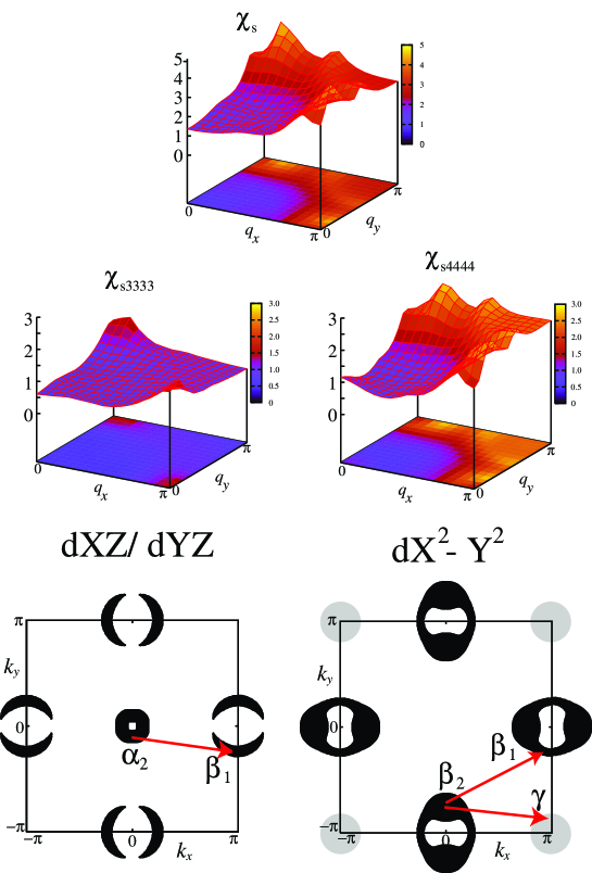
Figure 3: Top panel: Five-band RPA result for the spin susceptibility $\chi_{s}$ for $U=1.2$, $U^{\prime}=0.9$, $J=J^{\prime}=0.15$, $n=6.1$ and $T=0.02$ (in eV). Middle panels: Diagonal components, $\chi_{s3333}$(left) and $\chi_{s4444}$(right), of the spin susceptibility matrix in the orbital representation ($3:YZ,4:X^{2}-Y^{2}$). Bottom panel: Nesting is shown for the Fermi surface for orbitals $XZ,YZ$ (left) and for $X^{2}-Y^{2}$ (right). Here the thickness of the Fermi surface represents the strength of the respective orbital character. The gray areas around the corners in the left panel indicates the $\gamma$ “quasi” Fermi surface.

Let us first look at the key ingredient: the spin susceptibility in the top panel of Fig.3. The susceptibility $\chi_{s}$ has peaks around $(k_{x},k_{y})=(\pi,0)$, $(0,\pi)$. In addition we note that there is a ridge extending from $(\pi,\pi/2)$ to $(\pi/2,\pi)$ around $(\pi,\pi)$. To explore the origin of these spin structures, we show $\chi_{s3333}$ and $\chi_{s4444}$ in the middle of Fig.3, which represent the spin correlation within $d_{YZ}$ and $d_{X^{2}-Y^{2}}$ orbitals, respectively. $\chi_{s3333}$ peaks solely around $(\pi,0)$ and $(0,\pi)$, which reflects the nesting between the $XZ,YZ$-charactered portions of $\alpha$ and $\beta$ Fermi pockets as shown in a bottom panel of Fig.3. On the other hand, $\chi_{s4444}$ has peaks around $(\pi,0),(0,\pi)$ and around $(\pi,\pi/2)/(\pi/2,\pi)$ as well. The former is due to the nesting between the $\gamma$ quasi Fermi surface and the $d_{X^{2}-Y^{2}}$ portion of the $\beta$ Fermi surface as was first pointed out in ref.[4], while the latter originates from the nesting between the $d_{X^{2}-Y^{2}}$ portion of the $\beta_{1}$ and $\beta_{2}$ Fermi surfaces.[3] The $(\pi,0),(0,\pi)$ feature is consistent with the stripe (i.e., collinear) antiferromagnetic order for the undoped case, which was suggested by transport and optical reflectance,[19] and further confirmed by neutron scattering experiments.[7] The stabilization of such an antiferromagnetic ordering has also been pointed out in first principles calculations.[12, 19, 20]

5 Result: superconductivity

The presence of multiple set of nesting vectors revealed above provides an interesting case of the gap function in a spin-fluctuation mediated superconductivity, since multiple nestings can not only cooperate but also compete with each other. Namely, the $\alpha$-$\beta$ and $\gamma$-$\beta$ nestings tend to favour the sign reversing $s$-wave pairing, in which the gap changes sign between $\alpha$ and $\beta$ with a fixed sign (i.e., full gap) on each of the Fermi surface.[4] On the other hand, $\beta_{1}-\beta_{2}$ nesting tends to change the sign of the gap between these two pockets, which can result in either $d$-wave pairing or an $s$-wave pairing with nodes on the $\beta$ Fermi surface[21, 22]. For the band structure of LaFeAsO (obtained by using the experimentally determined lattice structure), the $(\pi,0)$ spin fluctuation dominates, and the sign-reversing $s$-wave with no nodes on the Fermi pockets dominates for the present set of parameter values.[22] In Fig.4, we show the gap function in the band representation for the third and the forth bands, which produce the $\alpha_{2}$ and $\beta$ Fermi surfaces, respectively. A number of theoretical studies that adopt effective two band models, [23, 24, 25] the present five band model,[26, 27, 28] or a 16 band $dp$ model[29] have also found that this sign reversing $s$-wave is a good candidate of the gap function in this material. The sign change in the $s$-wave gap is analogous to those in models studied by Bulut et al.,[30] and also by the present author for the disconnected Fermi surfaces[31, 32]. It is also reminiscent of the unconventional $s$-wave pairing mechanism for Na_xCoO${}_{2}\cdot y$H₂O[33] proposed by Kuroki et al.[34]

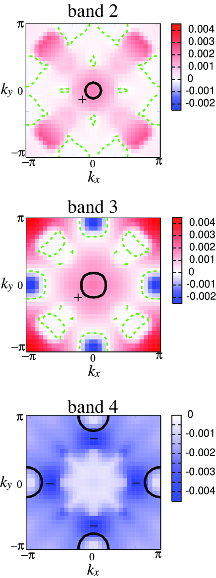
Figure 4: Gap function in the band representation for band 2 (top) band 3 (middle) and band 4 for the same set of parameter values as in Fig.3.

We have to realise, however, that the gap can vary significantly along the $\beta$ Fermi surface, and also between different pieces of the Fermi surface due to the multiorbital character of the system. In the present case, the gap for the $d_{X^{2}-Y^{2}}$-charactered portion of the $\beta$ Fermi surface is about twice as large as that for the $XZ,YZ$-charactered portions, namely near the Brillouin zone edge of the $\beta$ Fermi surface and on the $\alpha_{1}$, $\alpha_{2}$ Fermi surface. However, we find, in further calculations, that this gap variance is not universal, and depends strongly on the electron density and also on the details of the band structure. This is because the $\beta-\gamma$ nesting and thus the $(\pi,0)$ vs. $(\pi,\pi/2)$ spin fluctuation competition is sensitively affected by the position of the $d_{X^{2}-Y^{2}}$ portion of the band near $(\pi,\pi)$ with respect to the Fermi level. The details of this band filling and band structure dependences will be published elsewhere.

6 Conclusion

To summarise, we have constructed a five-band electronic model for LaFeAsO_1-xF_x, which we consider to be the minimum microscopic model for the iron-based superconductor. Applying a five-band RPA to this model, we have found that spin-fluctuation modes around $(\pi,0),(0,\pi)$ develop due to the nesting between disconnected Fermi surfaces. Based on the linearised Eliashberg equation, we have concluded that multiple spin fluctuation modes realises unconventional, extended $s$-wave pairing, where the gap changes sign across the nesting vectors.

So the general picture obtained here is that the iron compound is a multi-band system having electron and hole pockets, as sharply opposed to the cuprate which is a one-band and nearly half-filled system with a simply connected Fermi surface. This poses a challenging future problem of elaborating respective pros and cons for the iron compound and the cuprate for superconductivity.

References

- [1] Y.Kamihara, T.Watanabe, M.Hirano, H. Hosono: J. Am. Chem. Soc. 130 (2008) 3296.
- [2] Z.-A Ren, W. Lu, J. Yang, W. Yi, X.-L. Shen, Z.-C. Li, G.-C. Che, X.-L Dong, L.-L. Sun, F. Zhou, Z.-X. Zhao: Chin. Phys. Lett. 25 (2008) 2215.
- [3] K. Kuroki, S. Onari, R. Arita, H. Usui, Y. Tanaka, H. Kontani, and H. Aoki : Phys. Rev. Lett. 101 (2008) 087004.
- [4] I.I. Mazin, D.J. Singh, M.D. Johannes, M.H. Du:: Phys. Rev. Lett. 101 (2008) 057003.
- [5] H. Aoki, Physica C 437-438, 11 (2006); H Aoki in Condensed Matter Theories 21 ed. by H. Akai et al, (Nova Science, 2007).
- [6] This is in accord with a general tendency that 2D systems are more favourable than 3D systems for the spin-fluctuation mediated superconductivity as discussed by R. Arita, K. Kuroki and H. Aoki, Phys. Rev. B 60 (1999) 14585; J. Phys. Soc. Jpn. 69, 1181 (2000); P. Monthoux and G. G. Lonzarich, Phys. Rev. B 59, 14598 (1999).
- [7] C.de la Cruz, Q. Huang, J. W. Lynn, Jiying Li, W. Ratcliff II, J. L. Zarestky, H. A. Mook, G. F. Chen, J. L. Luo, N. L. Wang, P. Dai: Nature 453 (2008) 899.
- [8] S. Baroni, A. Dal Corso, S. de Gironcoli, P. Giannozzi, C. Cavazzoni, G. Ballabio, S. Scandolo, G. Chiarotti, P. Focher, A. Pasquarello, K. Laasonen, A. Trave, R. Car, N. Marzari, A. Kokalj, http://www.pwscf.org/. Here we adopt the exchange correlation functional introduced by J. P. Perdew, K. Burke, and Y. Wang [Phys. Rev. B 54 (1996) 16533], and the wave functions are expanded by plane waves up to a cutoff energy of 40 Ry. 103 -point meshes are used with the special points technique by H.J. Monkhorst and J.D. Pack [Phys. Rev. B 13 (1976) 5188 ].
- [9] N. Marzari and D. Vanderbilt: Phys. Rev. B 56 (1997) 12847; I. Souza, N. Marzari and D. Vanderbilt: Phys. Rev. B 65 (2002) 035109. The Wannier functions are generated by the code developed by A. A. Mostofi, J. R. Yates, N. Marzari, I. Souza and D. Vanderbilt, (http://www.wannier.org/) for the energy window eV 2.6 eV, where is the eigenenergy of the Bloch states and the Fermi energy.
- [10] While an ambiguity exists in unfolding the Brillouin zone [if the sign of the hoppings with =odd (i.e., hoppings between A and B sites in a bipartite lattice) is changed, a band structure is reflected with respect to ], this is just a unitary transformation, and either way the five-band structure gives the same ten bands in the folded Brillouin zone as well as the same RPA results.
- [11] D.J. Singh and M.-H. Du: Phys. Rev. Lett. 100 (2008) 237003.
- [12] S. Ishibashi, K. Terakura, H. Hosono: J. Phys. Soc. Jpn. 77 (2008) 053709.
- [13] H. Fukuyama: J. Phys. Soc. Jpn., online-news and comments [May 12, 2008].
- [14] K.Nakamura, R.Arita, M.Imada: J. Phys. Soc. Jpn. 77 (2008) 093711.
- [15] T. Miyake, L. Pourovskii, V. Vildosola, S. Biermann, A. Georges: J. Phys. Soc. Jpn. 77 (2008) Suppl. C 99.
- [16] V. I. Anisimov, Dm. M. Korotin, M. A. Korotin, A. V. Kozhevnikov, J. Kunes A. O. Shorikov, S. L. Skornyakov, S. V. Streltsov: arXiv: 0810.2629.
- [17] K. Yada and H. Kontani: J. Phys. Soc. Jpn. 74 (2005) 2161.
- [18] T. Takimoto, T. Hotta, and K. Ueda: Phys. Rev. B 69 (2004) 104504.
- [19] J. Dong, H.J. Zhang, G. Xu, Z. Li, W.Z. Hu, D. Wu, G.F.Chen, X. Dai, J.L. Luo, Z.Fang, and N.L.Wang: Europhys. Lett. 83 (2008) 27006.
- [20] I.I. Mazin, M.D. Johannes, L. Boeri, K. Koepernik, D.J. Singh: Phys. Rev. B 78 (2008) 085104.
- [21] S.Graser, T.A. Maier, P.J. Hirshfeld, and D.J. Scalapino : Phys. Rev. B 77 (2008) 180514.
- [22] In our previous paper[3] the gap function (diagonal element) of the 4th band had nodes intersecting the Fermi surface. This was in fact due to a technical error in the final stage of the calculation, i.e., the unitary transformation from the orbital to the band representations. However, the main conclusions of Ref.[3] do remain unaltered, since (i) the magnitude of the gap along the Fermi surface varies significantly as mentioned here, and (ii) the coexistence of and spin fluctuations determines the way in which nodes appear as asserted in [3]. The nodes of the gap function do intersect for certain choices of the parameter values or a slight change in the band structure, as shown in ref.[21].
- [23] X.-L. Qi, S. Raghu, C.-X. Liu, D.J.Scalapino, and S.C. Zhang : arXiv: 0804.4332.
- [24] Daghofer, A. Moreo, J. A. Riera, E. Arrigoni, D.J. Scalapino, E. Dagotto: Phys. Rev. Lett. 101 (2008) 237004.
- [25] A.V.Chubukov, V.Efremov, and I.Eremin: Phys. Rev. B 78 (2008) 134512.
- [26] T. Nomura: J. Phys. Soc. Jpn. 77 (2008) Suppl. C 123.
- [27] H. Ikeda: J. Phys. Soc. Jpn. 77 (2008) 123707.
- [28] F. Wang, H. Zhai, Y. Ran, A. Vishwanath, D.-H. Lee: Phys. Rev. Lett. 102 (2009) 047005.
- [29] Y.Yanagi, Y. Yamakawa, Y. Ono: J. Phys. Soc. Jpn. 77 (2008) 123701.
- [30] N. Bulut, D.J. Scalapino, and R.T. Scalettar : Phys. Rev. B 45 (1992) 5577.
- [31] K. Kuroki and R. Arita: Phys. Rev. B 64 (2001) 024501.
- [32] K. Kuroki, T. Kimura, and R. Arita: Phys. Rev. B 66 (2002) 184508.
- [33] K. Takada, H. Sakurai, E. Takayama-Muromachi, F. Izumi, R. Dilanian, and T. Sasaki: Nature 422 (2003) 53.
- [34] K. Kuroki, S. Onari, Y. Tanaka, R. Arita, and T. Nojima: Phys. Rev. B 73 (2006) 184503.