Survey of Planetary Nebulae at 30 GHz with OCRA-p

Abstract

Aims. We report the results of a survey of 442 planetary nebulae at 30 GHz. The purpose of the survey is to develop a list of planetary nebulae as calibration sources which could be used for high frequency calibration in future. For 41 PNe with sufficient data, we test the emission mechanisms in order to evaluate whether or not spinning dust plays an important role in their spectra at 30 GHz.

Methods. The 30-GHz data were obtained with a twin-beam differencing radiometer, OCRA-p, which is in operation on the Toruń 32-m telescope. Sources were scanned both in right ascension and declination. We estimated flux densities at 30 GHz using a free-free emission model and compared it with our data.

Results. The primary result is a catalogue containing the flux densities of 93 planetary nebulae at 30 GHz. Sources with sufficient data were compared with a spectral model of free-free emission. The model shows that free-free emission can generally explain the observed flux densities at 30 GHz thus no other emission mechanism is needed to account for the high frequency spectra.

1 Introduction

The planetary nebula (PN) phase in the evolution of low mass stars lasts only about $10^{4}$ years. It begins once the central star reaches an effective temperature of 20 000 K and ionises the shell of material developed during Asymptotic Giant Branch (AGB) evolution. The end of this phase is defined by termination of nuclear burning in a thin outer shell of the star, and then rapid dispersal of the nebula. At radio wavelengths, planetary nebulae emit continuum radiation in a free-free process and are among the brightest Galactic radio sources. Their radio flux densities do not suffer the high levels of extinction present in the optical regime. Since most planetary nebulae occupy Galactic plane where extinction is high, radio detections and radio flux density measurements are important.

Planetary nebulae are mostly compact sources because they are distant or intrinsically small. Their relatively strong and stable radio emission makes them good candidates for calibration sources.

Many radio continuum observations of planetary nebulae have been made at 1.4, 5 and 14.7 GHz (see Condon & Kaplan 1998; Acker et al. 1994; Aaquist & Kwok 1990; Milne & Aller 1982). There is still only limited data at frequencies above 30 GHz and most of those observations were obtained with interferometers such as the VLA; relatively little comes from single dishes. To extend the spectral range and to make total flux density measurements, we have used the new One Centimetre Radio Array prototype (OCRA-p) receiver to observe planetary nebulae at 30 GHz. This receiver is mounted on Toruń’s 32-m radio telescope and is described in section 2. OCRA-p receiver is outlined in detail by Lowe (2005). The survey for planetary nebulae was one of the first successful observations made using this system (together with measurements of flat-spectrum sources by Lowe et al. 2007, and observations of the Sunayaev Zel’dovich effect by Lancaster et al. 2007). The purpose was to make a list of high frequency calibrators, which can be used to support sky surveys and to test the emission mechanisms in order to evaluate whether or not spinning dust plays an important role in PN spectra.

Our new survey of planetary nebulae brought detections of 93 sources at 30 GHz out of 442, of which selection criteria are described in section 3. The observing techniques and data reduction process are described in section 3. The results are described in section 4. The comparison of flux densities with the free-free emission model proposed by Siódmiak & Tylenda (2001) is described in section 5. Section 6 contains the final conclusions. The measured 30-GHz flux densities of all detected PNe are given in Table LABEL:table1.

2 OCRA-p

OCRA-p is a 2-element prototype for OCRA (Browne et al. 2000) - a 100-element array receiver. The OCRA-p receiver was constructed at the University of Manchester and was funded by a EU Faraday FP6 grant together with the Royal Society Paul Instrument fund. It has been mounted on the Toruń 32-m radio telescope owned by the Centre for Astronomy, Nicolaus Copernicus University, Toruń in Poland.

Table 1: OCRA-p nominal system specification (from Lowe et al. 2007)

$$\begin{array}[]{p{0.5\linewidth}l}\hline\cr\vskip 3.0pt plus 1.0pt minus 1.0pt\cr\leavevmode\nobreak\ \leavevmode\nobreak\ \leavevmode\nobreak\ Frequency range&27-33\,\mathrm{GHz}\nobreak\leavevmode\nobreak\leavevmode\\ \leavevmode\nobreak\ \leavevmode\nobreak\ \leavevmode\nobreak\ System temperature&40\,\mathrm{K}\nobreak\leavevmode\nobreak\leavevmode\\ \leavevmode\nobreak\ \leavevmode\nobreak\ \leavevmode\nobreak\ Individual beam FWHM&1.2\,\mathrm{arcmin}\nobreak\leavevmode\nobreak\leavevmode\\ \leavevmode\nobreak\ \leavevmode\nobreak\ \leavevmode\nobreak\ Beam spacing&3.1\,\mathrm{arcmin}\nobreak\leavevmode\nobreak\leavevmode\\ \vskip 3.0pt plus 1.0pt minus 1.0pt\cr\hline\cr\end{array}$$

The basic OCRA design was based on the prototype demonstrator for the Planck Low Frequency Instrument (Mandolesi et al. 2000) and is similar to the K-band receivers mounted on the WMAP spacecraft (Jarosik et al. 2003). The nominal system specification is presented in Table 1. OCRA-p has two closely spaced feeds in the secondary focus of the 32 m telescope and thus there is very similar atmospheric emission in each beam. The basic observing mode with this radiometer involve switching continuously between the two horns and between two states of a 277$-Hz$ phase switch (0 and 180^o), located in one arm of the receiver. The switching frequency is much greater than the characteristic frequencies of atmospheric and gain fluctuations and those effects are dramatically reduced by taking differences between switch states and channels. The result, so-called double difference, is the observable used for data reduction. More details and an illustration of our scan strategy can be found in Lowe et al. (2007).

The full 100-beam OCRA receiver could be ideal for studying radio sources at higher frequencies, especially it is ideally suited to fast sky surveys.

3 Observations and data reduction

The observations were made over a period of 1.5 years, starting in December 2005. For a survey we selected 442 planetary nebulae from the Strasbourg-ESO Catalogue of Galactic Planetary Nebulae (Acker et al. 1994) having 5 GHz observations and declinations above $-15^{o}$.

A single flux density measurement consisted of two orthogonal scans with the first one made in elevation. Real-time software fitted a Gaussian profile to the observed beam shape and the measured position offset was used to update the telescope pointing corrections for the subsequent azimuthal scan. These corrections of pointing accuracy led to reliable estimate of flux density using the azimuthal scans. The first step of the data reduction was to fit a quadratic background baseline, subtract it from the data and fit double Gaussians to the azimuthal scan to ensure that the source is passing through each beam in turn. The quality of the data was strongly dependent on the weather conditions. During bad weather large asymmetries would be observed in the fitted amplitudes of the two beams. Data with differences in amplitudes exceeding 10% were not used. To fix the flux scale, NGC 7027 was used as the calibrator for the whole survey. It is the brightest planetary nebula in the radio sky due to its proximity and youth. It is a compact nebula of 10x13.5 arcsec (Atherton et al. 1979) observed regularly at the VLA for 25 years and can be taken to be unresolved when observed with the 1.2 arcmin beam of the 32 m telescope. Those features make NGC 7027 a good prime calibrator over a wide frequency range. Fortunately, at Toruń’s latitude the source is circumpolar so it could be observed at any time during the survey.

On human time scales the flux evolution of NGC 7027 is slow but it is measurable. Perley et al. (2006) suggest that the observed smooth decline of PNe flux densities at high frequencies is due to the reduction in the number of ionising photons with time. This is caused by evolution of the central star, whose temperature is increasing and luminosity is slowly decreasing. Measurements by Zijlstra et al. (2008) show that the flux density of NGC 7027 is decreasing at a rate of -7.79 mJy/yr at 30 GHz. Using this secular decrease in flux density, along with a flux density of 5433.8 mJy at 2000.0 based on VLA measurements in seven bands, we calculate a flux density for 2006.0 of 5.39$\pm$0.28 Jy. The data for all observed nebulae were scaled to this value.

The final results were corrected for gain-elevation curve of the telescope with elevation (a factor of up to 20%, depending of elevation). The atmospheric absorption was also taken into account. The final flux density uncertainty arising from double Gaussian fitting, calibrator uncertainty and all other corrections is about 8%.

4 Results

The final results are presented in Table LABEL:table1. The first column contains the SESO IAU Planetary Nebula in Galactic coordinates (PNG) name lll.l$\pm$bb.b, where lll.l is Galactic longitude and bb.b is Galactic latitude. The second column contains the normal descriptive designation. Coordinates for J2000, taken from Acker et al. (1994), are given in columns 3 and 4. Columns 5 and 6 contain the measured flux densities at 30 GHz and calculated uncertainties. The values marked by $\ast$ are sources with optical angular size larger that 1/4 OCRA-p beam, while those marked by $\Delta$ are corrected using adopted angular diameter which can be found only for some sources (see section 5). Table LABEL:table1 contains data for 93 sources. Figure 7 presents PN modeled radio spectra (see section 5) together with flux densities at 1.4, 5, 14.7 GHz.

The distribution of detected flux densities in presented in Figure 1. It is seen that there is an instrumental limit on the detectability of sources around 20 mJy. The exact value depends on the weather conditions at the time of observations.

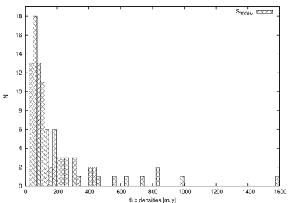
Figure 1: Histogram of the distribution of measured planetary nebulae flux densities at 30 GHz.

5 Analysis of flux density results

The first result of the survey is a new catalogue of 93 Planetary Nebulae flux densities at a frequency of 30 GHz. We have plotted in Figure 2 a histogram for the distances of all PNe surveyed in this work, and marking those detected by OCRA-p. The data was taken from the Strasbourg-ESO Catalogue of Galactic Planetary Nebulae. Histogram shows that we were able to measure planetary nebulae flux densities at distances out to about 5 kpc and that the distributions of detected and non-detected PNe in our data are similar.

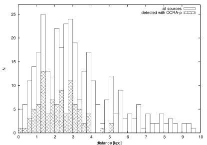
Figure 2: Histogram of the distribution of planetary nebulae distances. The plot presents distances to all planetary nebulae examined in the survey and the ones detected by OCRA-p are highlighted.

Planetary nebulae are strong infrared sources and it is known that they occupy certain characteristic positions on the IRAS colour-colour diagram. Pottasch et al. (1988) made IRAS measurements of over 300 planetary nebulae in 4 bands: 12 $\mathrm{\mu m}$, 25 $\mathrm{\mu m}$, 60 $\mathrm{\mu m}$ and 100 $\mathrm{\mu m}$. We used the first three to construct a useful colour-colour diagram. Figure 3 shows this diagram for all examined sources and the ones detected with OCRA-p. It can be seen that planetary nebulae measured by OCRA are concentrated close to the black-body (120-180 K) line in the plot. This is due to the evolution of planetary nebula. As the dust cools with time, the dust colours will redden whilst the nebulae becomes less opaque in the radio region, resulting in an increase in radio emission. Thus observed radio emission provides useful hints on planetary nebulae evolution.

Figure 3: The distribution of planetary nebulae in the colour-colour diagram, showing all sources examined in the survey and those detected by OCRA-p. The line indicates IRAS colours for a black body distribution with temperatures from 100 K up to 700 K, with 100 K steps marked by dots.

Planetary nebula emission at 30 GHz is thought to be due to free-free emission. We want to check whether this mechanism can fully explain the measured flux densities since there have been claims that the excess emission has been seen in planetary nebulae (Casassus et al. 2004). A model of planetary nebula free-free emission was taken from Siódmiak & Tylenda (2001). These authors analysed the flux densities of 264 planetary nebulae with reliable measurements at 1.4 and 5 GHz and known diameters (with radio diameter defined by radio contours at 10% of the peak flux density, or the mean value of optical and radio diameter). Four simple models were proposed and examined. The most reasonable approach is to consider a model consisting of two regions with different optical depth. Each source is then modelled a dense region which fills a solid angle $\xi\Omega$ characterised by optical depth $\tau_{\nu}$, and a less dense region filling up $(1-\xi)\Omega$ described by optical depth $\epsilon\tau_{\nu}$. With such an assumption one can model the spectra of all PNe, including the small fraction of the population which are homogeneous and symmetric.

The observed flux density is then expressed as:

$$S_{\nu}=\frac{2\nu^{2}kT_{e}}{c^{2}}\left({\left({1-e^{-\tau_{\nu}}}\right)\xi\Omega+\left({1-e^{-\epsilon\tau_{\nu}}}\right)(1-\xi)\Omega}\right),$$ (1)

where the optical thickness depends on the frequency $\nu$ roughly as (see Pottasch 1984):

$$\tau_{\nu}=\tau_{0}(\nu/\nu_{0})^{-2.1}.$$ (2)

$\tau_{0}$ and $\nu_{0}$ (=5 GHz) are the reference optical thickness and frequency. Optical thickness at 5 GHz is found by solving the first expression with known flux density at this frequency.

The best fit values found by Siódmiak & Tylenda (2001) from their population as a whole were $\xi=0.27$ and $\epsilon=0.19$. The model assumes that entire nebula has the same electron temperature, $T_{e}$. The values of $T_{e}$ were calculated based on measurements of HeII$\lambda$4686Å   taken from Tylenda et al. (1994) and the method described by Kaler (1986). With this knowledge we can count modeled flux density at 30 GHz.

Several data sets are required to apply the model described above. HeII$\lambda$4686Å line intensities were taken from Tylenda et al. (1994), 5 GHz radio flux densities from Acker et al. (1994), 1.4 GHz flux densities from Condon & Kaplan (1998) and adopted angular diameters from Siódmiak & Tylenda (2001). 5 GHz and 30 GHz flux density data are from single-dish measurements. This is important because, as noticed by Zijlstra et al. (1989), observed flux densities from a single dish are systematically higher than from an interferometer, which is insensitive to the extended, ionised halo emission. The data required for the model are available for 41 objects out of the 93 for which we have reliable 30 GHz flux densities and for these sources the emission model can be tested. If source was extended in comparison to OCRA-p beam, the adopted angular diameters were used to correct measured flux densities. We assumed that PN are spherical sources with the given diameter and with constant surface brightness. This was a case of only 3 sources: NGC2438, NGC7008, NGC6781. Table LABEL:table1 contains corrected values.

In Figure 4 we compare the observed and modeled 30 GHz flux densities. The model generally agrees well with the measured values. The dependence of the logarithm of the observed to modeled flux densities at 30 GHz on electron temperature and brightness temperature (derived from flux density at 5 GHz - $S_{5\,GHz}$ and PNe diameter - $\Theta$ using $T_{b}=73.87\cdot S_{5\,GHz}/{\Theta^{2}}$) is presented in Figures 5 and 6. As can be seen, the differences between observed and modeled values are small and independent of $T_{e}$ or $T_{b}$ parameters.

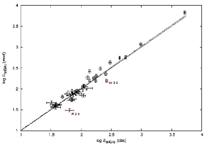
Figure 4: Modeled versus observed flux density at 30 GHz. The solid line indicates these flux densities being equal, while the dashed line represents the best straight-line fit to relationship between $log\,S_{30GHz}\,(mod)$ and $log\,S_{30GHz}\,(obs)$.

Figure 5: Observed to modeled flux density ratio at 30 GHz versus electron temperature.

Figure 6: Observed to modeled flux density ratio at 30 GHz versus brightness temperature.

Most of the data is in good agreement with the model, despite its simplicity, so that our observations can be generally explained by the free-free emission mechanism with no requirement for an additional emission mechanism. However, there are two sources, M 2-9 (010.8+18.0) and Vy2-2 (058.3-10.9), in which it can be seen that the observed flux density is significantly higher than the value expected from the model.

M 2-9 is a planetary nebula known for its additional emission at higher frequencies (see Figure 7). This emission was explained by Kwok et al. (1985) and Davis et al. (1979) as the result of an optically thick stellar wind, which is the dominant emission source above about 20 GHz. The high mass loss from the central star was discovered by Swings & Andrillat (1979) on the basis of their analysis of its broad H$\alpha$ line. The observed 30 GHz point shows that the stellar wind is optically thick above 30 GHz.

Vy 2-2 (see Figure 7) is a young and compact nebula. It is characterised by bright IR emission, a large optical depth at radio frequencies and faint emission. Its turnover frequency is much greater than 10 GHz so the assumption of optically thin emission at 5 GHz made by our model is not well fulfilled and therefore a disagreement with the model is not unexpected.

Another source which should be mentioned is Hu 1-2 (086.5-08.8) (see Figure 7) where emission at 30 GHz is a below the expected value. However a check of the other spectral measurements of this nebula suggest that the point at 5 GHz is overestimated.

The model was constructed to check whether any mechanism other than free-free emission is needed to explain the spectra of planetary nebulae at 30 GHz, as suggested by Casassus et al. (2007). Such an excess was found at 10-30 GHz in the spectral energy distribution (SED) of sources such as the dark cloud LDN 1622 (Finkbeiner 2004), an H II region in Perseus (Watson et al. 2005) and the Helix nebula (Casassus et al. 2004). Draine & Lazarian (1998) suggest that radiation from spinning electric dipoles created by very small grains (VSGs) or spinning dust is responsible for the observed excess. Yet in our data the effect is not observed. This conclusion is in agreement with new observations of planetary nebulae at 43 GHz (Umana et al. 2008), whose measurements are mostly in agreement within errors with those presented in this paper (with exception for PN IC2165 (221.3-12.3)).

6 Conclusions

We surveyed 442 planetary nebulae from 5-GHz catalogue of Acker et al. (1994) with declinations above $-15^{o}$. 93 sources were detected above 23 mJy and their flux densities at 30 GHz were measured and presented in this paper. The model for free-free emission described by Siódmiak & Tylenda (2001) was used to predict 30 GHz flux densities based on the 5 GHz observations and the known diameters. These calculated values are in good agreement with the observed flux densities. No additional emission mechanism is needed to explain the observed spectra.

Table 5: 30 GHz survey.; col. (1) gives the SESO IAU Planetary Nebula in Galactic coordinates (PNG) name lll.l$\pm$bb.b, where lll.l is Galactic longitude and bb.b is Galactic latitude. The values marked by $\ast$ are sources with optical angular size larger that 1/4 OCRA-p beam, while those marked by $\Delta$ are corrected using adopted angular diameter (see section 5).; col. (2) gives the normal descriptive designation, cols. (3) and (4) give coordinates for J2000, taken from Acker et al. (1994); cols. (5) and (6) give measured flux densities at 30 GHz and calculated uncertainties.

PNG	Name	R.A. (J2000)	Declination (J2000)	$S_{30GHz}$ (mJy)	$\Delta S_{30GHz}$ (mJy)
(1)	(2)	(3)	(4)	(5)	(6)
010.8+18.0	M 2-9	17 05 37.952	-10 08 34.58	63.8	9.9
015.9+03.3	M 1-39	18 07 30.699	-13 28 47.61	70	11
019.4-05.3	M 1-61	18 45 55.072	-14 27 37.93	127	27
019.7+03.2	M 3-25	18 15 16.967	-10 10 09.47	76.8	8.0
020.9-01.1	M 1-51	18 33 28.943	-11 07 26.41	229.9	7.4
023.9-02.3	M 1-59	18 43 20.178	-09 04 48.64	107	15
025.3+40.8	IC 4593	16 11 44.544	+12 04 17.06	66.8	4.8
025.8-17.9	NGC 6818	19 43 57.844	-14 09 11.91	208	30
027.6+04.2	M 2-43	18 26 40.048	-02 42 57.63	259	10
027.7+00.7	M 2-45	18 39 21.837	-04 19 50.90	158	17
031.0+04.1	K 3-6	18 33 17.490	+00 11 47.19	98.6	8.3
032.7-02.0	M 1-66	18 58 26.247	-01 03 45.70	68.7	9.6
034.0+02.2	K 3-13	18 45 24.582	+02 01 23.85	91.3	7.1
034.6+11.8	NGC 6572	18 12 06.365	+06 51 13.01	987	38
035.1-00.7	Ap 2-1	18 58 10.459	+01 36 57.15	241	13
037.7-34.5	NGC 7009	21 04 10.877	-11 21 48.25	470	21
037.8-06.3	NGC 6790	19 22 56.965	+01 30 46.45	303	12
038.2+12.0	Cn 3-1	18 17 34.104	+10 09 03.34	68.6	6.4
039.8+02.1	K 3-17	18 56 18.171	+07 07 26.31	303	9.0
040.3-00.4	A 53	19 06 45.910	+06 23 52.47	54.9	6.5
041.8-02.9Δ	NGC 6781	19 18 28.085	+06 32 19.29	264.1	7.1
043.1+37.7	NGC 6210	16 44 29.491	+23 47 59.68	225.7	8.1
045.4-02.7	Vy 2-2	19 24 22.229	+09 53 56.66	266	12
045.7-04.5	NGC 6804	19 31 35.175	+09 13 32.01	78.1	6.6
046.4-04.1	NGC 6803	19 31 16.490	+10 03 21.88	83.8	6.3
047.0+42.4*	A 39	16 27 33.737	+27 54 33.44	264	18
048.0-02.3	PB 10	19 28 14.391	+12 19 36.17	37.1	6.5
048.1+01.1	K 3-29	19 15 30.561	+14 03 49.83	71.2	5.8
048.5+04.2	K 4-16	19 04 51.471	+15 47 37.83	107	11
048.7+01.9	He 2-429	19 13 38.422	+14 59 19.21	62.1	6.1
050.1+03.3*	M 1-67	19 11 30.877	+16 51 38.16	102.8	6.1
051.0+03.0	He 2-430	19 14 04.197	+17 31 32.92	37.7	6.7
051.4+09.6	Hu 2-1	18 49 47.565	+20 50 39.34	111.7	5.5
051.9-03.8	M 1-73	19 41 09.323	+14 56 59.37	36.5	4.8
054.1-12.1	NGC 6891	20 15 08.838	+12 42 15.63	97.2	7.3
055.5-00.5	M 1-71	19 36 26.927	+19 42 23.99	178.9	6.3
056.0+02.0	K 3-35	19 27 44.036	+21 30 03.83	60.1	6.4
057.9-01.5	He 2-447	19 45 22.164	+21 20 04.03	65.5	7.1
058.3-10.9	IC 4997	20 20 08.741	+16 43 53.71	108.9	6.4
060.1-07.7	NGC 6886	20 12 42.813	+19 59 22.65	73.5	7.6
060.8-03.6*	NGC 6853	19 59 36.340	+22 43 16.09	95	11
061.4-09.5*	NGC 6905	20 22 22.940	+20 06 16.80	38.8	4.5
063.1+13.9*	NGC 6720	18 53 35.079	+33 01 45.03	189.7	7.0
064.7+05.0	BD+30 3639	19 34 45.232	+30 30 58.94	551	13
064.9-02.1	K 3-53	20 03 22.475	+27 00 54.73	73.8	5.3
067.9-00.2	K 3-52	20 03 11.435	+30 32 34.15	90.2	9.9
068.3-02.7	He 2-459	20 13 57.898	+29 33 55.94	102.5	6.9
069.7-00.0	K 3-55	20 06 56.210	+32 16 33.60	76.9	7.0
071.6-02.3	M 3-35	20 21 03.769	+32 29 23.86	161.8	6.4
074.5+02.1	NGC 6881	20 10 52.464	+37 24 41.18	109.1	7.4
075.7+35.8	Sa 4-1	17 13 50.35	+49 16 11.0	183.8	7.6
078.3-02.7	K 4-53	20 42 16.744	+37 40 25.58	44.4	6.3
082.1+07.0	NGC 6884	20 10 23.66	+46 27 39.8	139.3	6.8
083.5+12.7	NGC 6826	19 44 48.150	+50 31 30.26	303.5	8.2
086.5-08.8	Hu 1-2	21 33 08.349	+39 38 09.57	89.2	5.9
089.0+00.3	NGC 7026	21 06 18.209	+47 51 05.35	208.2	9.5
089.8-00.6	Sh 1-89	21 14 07.628	+47 46 22.17	831	45
089.8-05.1	IC 5117	21 32 31.027	+44 35 48.53	208.6	9.1
093.4+05.4Δ	NGC 7008	21 00 32.503	+54 32 36.18	178.1	8.1
093.5+01.4	M 1-78	21 20 44.809	+51 53 27.88	846	18
095.2+00.7	K 3-62	21 31 50.203	+52 33 51.64	101.3	7.8
096.4+29.9	NGC 6543	17 58 33.423	+66 37 59.52	630	15
097.5+03.1*	A 77	21 32 10.238	+55 52 42.67	409.3	9.8
100.0-08.7	Me 2-2	22 31 43.686	+47 48 03.96	32.1	5.6
100.6-05.4	IC 5217	22 23 55.725	+50 58 00.43	38.4	5.7
104.1+01.0	Bl 2-1	22 20 16.638	+58 14 16.59	45	4.6
106.5-17.6	NGC 7662	23 25 53.6	+42 32 06	435	13
107.8+02.3	NGC 7354	22 40 19.940	+61 17 08.10	439	13
110.1+01.9	PM 1-339	22 58 54.857	+61 57 57.77	31.4	4.1
111.8-02.8	Hb 12	23 26 14.814	+58 10 54.65	398.7	9.4
120.0+09.8*	NGC 40	00 13 01.015	+72 31 19.09	331.8	8.3
123.6+34.5	IC 3568	12 33 06.871	+82 33 48.95	58.3	5.4
130.2+01.3	IC 1747	01 57 35.896	+63 19 19.36	67.4	3.6
130.9-10.5*	NGC 650-51	01 42 19.948	+51 34 31.15	62.9	3.8
138.8+02.8	IC 289	03 10 19.273	+61 19 00.91	98.8	4.0
144.5+06.5*	NGC 1501	04 06 59.190	+60 55 14.34	136.2	3.8
147.4-02.3	M 1-4	03 41 43.428	+52 17 00.28	59.4	5.5
148.4+57.0*	NGC 3587	11 14 47.734	+55 01 08.50	23.1	3.6
161.2-14.8	IC 2003	03 56 21.984	+33 52 30.59	40	6.3
165.5-15.2*	NGC 1514	04 09 16.984	+30 46 33.47	59.6	3.2
166.1+10.4	IC 2149	05 56 23.908	+46 06 17.32	117.2	3.5
166.4-06.5	CRL 618	04 42 53.64	+36 06 53.4	731	20
173.7+02.7	PP 40	05 40 53.333	+35 42 22.29	173	4.9
184.0-02.1	M 1-5	05 46 50.000	+24 22 02.32	49.3	2.8
189.1+19.8*	NGC 2371-72	07 25 34.720	+29 29 25.63	25	3.9
194.2+02.5	J 900	06 25 57.275	+17 47 27.19	86.1	4.8
196.6-10.9	NGC 2022	05 42 06.229	+09 05 10.75	70.1	3.8
197.8+17.3	NGC 2392	07 29 10.767	+20 54 42.49	186.6	5.8
206.4-40.5	NGC 1535	04 14 15.762	-12 44 22.03	125.4	9.8
211.2-03.5	M 1-6	06 35 45.126	-00 05 37.36	95	7.6
215.2-24.2	IC 418	05 27 28.204	-12 41 50.26	1581	50
221.3-12.3	IC 2165	06 21 42.775	-12 59 13.96	173.6	7.9
231.8+04.1Δ	NGC 2438	07 41 51.426	-14 43 54.88	89	10

Table 5: continued.

Fig. 6: Radio spectra of PN with flux densities at 1.4, 5, 14.7 GHz from the literature (see Condon & Kaplan 1998; Acker et al. 1994; Aaquist & Kwok 1990; Milne & Aller 1982) and 30 GHz (OCRA-p) points from Table LABEL:table1, cols. (5) and (6).

Fig. 6: continued.