Entanglement signature in the mode structure of a single photon

Abstract

It is shown that entanglement, which is a quantum correlation property of at least two subsystems, is imprinted in the mode structure of a single photon. The photon, which is emitted by two coupled cavities, carries the information on the concurrence of the two intracavity fields. This can be useful for recording the entanglement dynamics of two cavity fields and for entanglement transfer.

An atom interacting with a quantized radiation-field mode in a high-$Q$ optical cavity plays an important role in quantum optics, for a review see, e.g., Ref. HarocheRaimond . The ability to coherently control individual quantum system, and in particular the quantum control of single-photon emission from an atom in a cavity, is a key requirement in various applications of quantum networks for distribution and processing of quantum information Cirac:3221 ; Brattke:3534 ; Knill:46 ; Monroe:238 ; Kimble:1023 . Recently, single-photon sources operating on the basis of adiabatic passage with just one atom trapped in a high-$Q$ optical cavity have been realized Parkins:3095 ; Hennrich:4872 ; Mckeever:1992 ; Hijlkema:253 . In this way, the adjustment of the spatiotemporal profile of single-photon pulses has been achieved Kuhn:067901 ; Keller:1075 . Moreover, the generation of single photons of known circular polarization emitted into a well-defined spatiotemporal mode has been possible Wilk:063601 , and an atom-photon quantum interface involving atom-photon entanglement has been realized Wilk:488 . More recently, the amplitude modulation in the photon emission on a single atom-cavity system has been studied theoretically Difidio:043822 and experimentally Bochmann:223601 . In addition, photon-photon entanglement with a single trapped atom in a high-finesse optical cavity has been performed Weber:030501 .

In the present contribution, in view of the widespread applications of cavity-assisted single-photon sources, we study single-photon emission from a system consisting of two coupled atom-cavity subsystems in a cascaded configuration Carmichael:2273 ; Gardiner:2269 . The mode structure of the radiated photon strongly depends on the entanglement between the two intracavity fields and it sensitively depends on the presence or absence of an atom in the second cavity. We show how the entanglement of the intracavity fields can be experimentally determined.

The system under study consists of two atom-cavity subsystems $A$ and $B$, where the source subsystem $A$ is cascaded with the target subsystem $B$, cf. Fig. 1. The cavities have three perfectly reflecting mirrors and one mirror with transmission coefficient $T\ll 1$. In the two subsystems $A$ and $B$ we consider a two-level atomic transition of frequency $\omega_{k}$ (related to the atomic energy eigenstates $|1_{k}\rangle$ and $|0_{k}\rangle$) coupled to a cavity mode of frequency $\omega_{k}^{\prime}$, where $k=a,b$ denotes the subsystem. The cavity mode is detuned by $\Delta_{k}$ from the two-level atomic transition frequency, $\omega_{k}=\omega_{k}^{\prime}+\Delta_{k}$, and is damped by losses through the partially transmitting cavity mirrors. In addition to the wanted outcoupling of the field, the photon can be spontaneously emitted out the side of the cavity into modes other than the one which is preferentially coupled to the resonator. Moreover, the photon may be absorbed or scattered by the cavity mirrors.

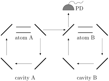
Figure 1: The cascaded system consists of two atom-cavity subsystems $A$ and $B$. A photodetector PD monitors the radiation field.

To describe the dynamics of the system we use the following master equation for the reduced density operator $\hat{\rho}(t)$ of the system:

$$\frac{d\hat{\rho}(t)}{dt} = \frac{1}{i\hbar}\!\left[\hat{H},\hat{\rho}(t)\right]\!+\!\sum_{i=1}^{5}\left[\hat{J}_{i}\hat{\rho}(t)\hat{J}_{i}^{\dagger}-\frac{1}{2}\hat{J}_{i}^{\dagger}\hat{J}_{i}\hat{\rho}(t)\right.$$ (1)

$$- \left.\frac{1}{2}\hat{\rho}(t)\hat{J}_{i}^{\dagger}\hat{J}_{i}\right].$$

The Hamiltonian is given by

$$\hat{H}=\hat{H}_{A}+\hat{H}_{B}+i\hbar\frac{\sqrt{\kappa_{a}\kappa_{b}}}{2}\left(e^{-i\phi}\hat{b}\hat{a}^{\dagger}-e^{i\phi}\hat{b}^{\dagger}\hat{a}\right)\,,$$ (2)

where $\hat{H}_{A}$ and $\hat{H}_{B}$ describe the atom-cavity interaction in the two subsystems $A$ and $B$, respectively, and, in the rotating-wave approximation, are given by

$$\hat{H}_{A}=\hbar g_{a}\left(\hat{a}\hat{A}_{10}+\hat{a}^{\dagger}\hat{A}_{01}\right)+\hbar\Delta_{a}{\hat{A}}_{11}\,,$$ (3)

and

$$\hat{H}_{B}=\hbar g_{b}\left(\hat{b}\hat{B}_{10}+\hat{b}^{\dagger}\hat{B}_{01}\right)+\hbar\Delta_{b}{\hat{B}}_{11}\,.$$ (4)

The third term in Eq. (2) describes the coupling between the two cavities Carmichael:2273 ; Gardiner:2269 . In these expressions, $\hat{a}$ ($\hat{a}^{\dagger}$) and $\hat{b}$ ($\hat{b}^{\dagger}$) are the annihilation (creation) operators for the cavity fields $A$ and $B$, respectively. We have also defined $\hat{A}_{ij}=|i_{a}\rangle\langle j_{a}|$ ($i,j=0,1$), and $\hat{B}_{ij}=|i_{b}\rangle\langle j_{b}|$ ($i,j=0,1$). In addition, $g_{k}$ is the atom-cavity coupling constant and $\kappa_{k}$ the cavity bandwidth, and the phase $\phi$ is related to the spatial separation between the source and the target, cf. Carmichael2 . The jump operators $\hat{J}_{i}$ are defined by

$$\hat{J}_{1}=\sqrt{\kappa_{a}}\hat{a}+\sqrt{\kappa_{b}}e^{-i\phi}\hat{b}\,,$$ (5)

which describes photon emission by the cavities;

$$\hat{J}_{2}=\sqrt{\kappa_{a}^{\prime}}\hat{a}\,,~{}~{}~{}~{}~{}~{}~{}\hat{J}_{3}=\sqrt{\kappa_{b}^{\prime}}\hat{b}\,,$$ (6)

are associated with photon absorption or scattering by the cavity mirrors; and

$$\hat{J}_{4}=\sqrt{\Gamma_{a}}\hat{A}_{01}\,,~{}~{}~{}~{}~{}~{}~{}\hat{J}_{5}=\sqrt{\Gamma_{b}}\hat{B}_{01}\,,$$ (7)

are related to spontaneous emission by the atoms. Here $\kappa_{k}^{\prime}$ and $\Gamma_{k}$ are the cavity mirrors’ absorption (or scattering) rate and the spontaneous emission rate of the two-level atom, respectively. Note that the operator $\hat{J}_{1}$ contains the superposition of the two fields radiated by the two cavities, due to the fact that the radiated photon cannot be associated with photon emission from either $A$ or $B$ separately.

To evaluate the time evolution of the system we use a quantum trajectory approach Carmichael2 ; Dalibard:580 ; Dum:4382 . Let us consider the system prepared at time $t_{0}=0$ in the state $|a\rangle\equiv|1,0,0,0\rangle$, which denotes the atom $A$ in the state $|1_{a}\rangle$, the cavity $A$ in the vacuum state, the atom $B$ in the state $|0_{b}\rangle$ , and the cavity $B$ in the vacuum state. Similarly, we define $|b\rangle\equiv|0,1,0,0\rangle$, $|c\rangle\equiv|0,0,1,0\rangle$, $|d\rangle\equiv|0,0,0,1\rangle$, and $|e\rangle\equiv|0,0,0,0\rangle$. To determine the state vector of the system at a later time $t$, assuming that no jump has occurred between time $t_{0}$ and $t$, we have to solve the nonunitary Schrödinger equation

$$i\hbar\frac{d}{dt}|\bar{\psi}_{\rm no}(t)\rangle=\hat{H^{{}^{\prime}}}\,|\bar{\psi}_{\rm no}(t)\rangle\,,$$ (8)

where $\hat{H^{{}^{\prime}}}$ is the non-Hermitian Hamiltonian given by

$$\hat{H^{{}^{\prime}}} = \hat{H}-\frac{i\hbar}{2}\sum_{i=1}^{5}\hat{J}_{i}^{\dagger}\hat{J}_{i}=\hat{H}_{A}+\hat{H}_{B}-i\hbar\Big{(}\frac{K_{a}}{2}\hat{a}^{\dagger}\hat{a}$$ (9)

$$+ \frac{K_{b}}{2}\hat{b}^{\dagger}\hat{b}+\frac{\Gamma_{a}}{2}\hat{A}_{11}+\frac{\Gamma_{b}}{2}\hat{B}_{11}+\sqrt{\kappa_{a}\kappa_{b}}e^{i\phi}\hat{b}^{\dagger}\hat{a}\Big{)},$$

where we have defined $K_{a}=\kappa_{a}+\kappa_{a}^{\prime}$ and $K_{b}=\kappa_{b}+\kappa_{b}^{\prime}$. If no jump has occurred between time $t_{0}$ and $t$, the system evolves via Eq. (8) into the unnormalized state

$$|\bar{\psi}_{\rm no}(t)\rangle=\alpha(t)|a\rangle+\beta(t)|b\rangle+\gamma(t)|c\rangle+\delta(t)|d\rangle\,.$$ (10)

The evolution governed by the nonunitary Schrödinger equation (8) is randomly interrupted by one of the five kinds of jumps $\hat{J}_{i}$, cf. Eqs. (5)-(7). If a jump has occurred at time $t_{\rm J}$, $t_{\rm J}\in(t_{0},t]$, the wave vector is found collapsed into the state $|e\rangle$ due to the action of one of the jump operators

$$\hat{J}_{i}\,|\bar{\psi}_{\rm no}(t_{\rm J})\rangle\rightarrow|e\rangle~{}~{}(i=1,\ldots,5).$$ (11)

In the problem under study we may have only one jump. Once the system collapses into the state $|e\rangle$, the nonunitary Schrödinger equation (8) lets it remain unchanged. The density operator $\hat{\rho}(t)$ is then obtained by performing an ensemble average over the different trajectories at time $t$, yielding the statistical mixture

$$\hat{\rho}(t)=|\bar{\psi}_{\rm no}(t)\rangle\langle\bar{\psi}_{\rm no}(t)|+|\epsilon(t)|^{2}|e\rangle\langle e|\,,$$ (12)

where $|\epsilon(t)|^{2}\equiv 1-\langle\bar{\psi}_{\rm no}(t)|\bar{\psi}_{\rm no}(t)\rangle$. The values $|\alpha(t)|^{2}$, $|\beta(t)|^{2}$, $|\gamma(t)|^{2}$, $|\delta(t)|^{2}$, and $|\epsilon(t)|^{2}$ represent the probabilities that at time $t$ the system can be found either in $|a\rangle$, $|b\rangle$, $|c\rangle$, $|d\rangle$, or $|e\rangle$, respectively.

In order to determine $\alpha(t)$, $\beta(t)$, $\gamma(t)$, and $\delta(t)$, we have to solve the nonunitary Schrödinger equation, cf. Eqs. (8) and (9), which leads to the inhomogeneous system of differential equations

$$\left\{\begin{array}[]{llll}\dot{\alpha}(t)=-i\left(\Delta_{a}-i\Gamma_{a}/2\right)\alpha(t)-ig_{a}\beta(t)\,,\\ \dot{\beta}(t)=-ig_{a}\alpha(t)-(K_{a}/2)\beta(t)\,,\\ \dot{\gamma}(t)=-i\left(\Delta_{b}-i\Gamma_{b}/2\right)\gamma(t)-ig_{b}\delta(t)\,,\\ \dot{\delta}(t)=-ig_{b}\gamma(t)-(K_{b}/2)\delta(t)-\sqrt{\kappa_{a}\kappa_{b}}e^{i\phi}\beta(t)\,.\end{array}\right.$$ (13)

For the initial conditions $\alpha(0)\!=\!1$, $\beta(0)\!=\!0$, $\gamma(0)\!=\!0$, and $\delta(0)\!=\!0$, and defining

$$\Omega_{k}\!\equiv\!\sqrt{\frac{K_{k}^{2}}{4}\!-\!4g_{k}^{2}\!-\!iK_{k}\!\left(\Delta_{k}\!-\!i\frac{\Gamma_{k}}{2}\right)\!-\!\left(\Delta_{k}\!-\!i\frac{\Gamma_{k}}{2}\right)^{2}}\,,$$ (14)

we get, similarly as done in Difidio:032334 , the solutions

$${\alpha}(t) = \left[\frac{K_{a}/2-i(\Delta_{a}-i\Gamma_{a}/2)}{\Omega_{a}}\sinh\!\left(\frac{\Omega_{a}t}{2}\right)\right.$$

$$+ \left.\cosh\!\left(\frac{\Omega_{a}t}{2}\right)\right]\!e^{-[(K_{a}+\Gamma_{a})/4+i\Delta_{a}/2]t},$$

$${\beta}(t) = -\frac{2ig_{a}}{\Omega_{a}}\sinh\!\left(\frac{\Omega_{a}t}{2}\right)e^{-[(K_{a}+\Gamma_{a})/4+i\Delta_{a}/2]t}\,,$$

$${\gamma}(t) = g_{b}\left\{f_{+}(t)\!\left[g_{-}(t)\!+\!h_{+}(t)\right]\!-\!f_{-}(t)\!\left[g_{+}(t)\!+\!h_{-}(t)\right]\right\},$$

$${\delta}(t) = i\!\left[\frac{K_{b}\!-\!\Gamma_{b}}{4}\!-\!i\frac{\Delta_{b}}{2}\!+\!\frac{\Omega_{b}}{2}\right]\!f_{-}(t)\!\left[g_{+}(t)\!+\!h_{-}(t)\right]$$ (15)

$$- i\!\left[\frac{K_{b}\!-\!\Gamma_{b}}{4}\!-\!i\frac{\Delta_{b}}{2}\!-\!\frac{\Omega_{b}}{2}\right]\!f_{+}(t)\!\left[g_{-}(t)\!+\!h_{+}(t)\right]\!.$$

Here we have defined,

$$f_{\pm}(t)=\frac{g_{a}\sqrt{\kappa_{a}\kappa_{b}}e^{i\phi}}{\Omega_{a}\Omega_{b}}e^{[-(K_{b}+\Gamma_{b})/4-i\Delta_{b}/2\pm\Omega_{b}/2]t}\,,$$ (16)

$$g_{\pm}(t)=\frac{e^{[(\Omega_{a}\pm\Omega_{b})/2-\Upsilon-i\Lambda]t}-1}{(\Omega_{a}\pm\Omega_{b})/2-\Upsilon-i\Lambda}\,,$$ (17)

and

$$h_{\pm}(t)=\frac{e^{-[(\Omega_{a}\pm\Omega_{b})/2+\Upsilon+i\Lambda]t}-1}{(\Omega_{a}\pm\Omega_{b})/2+\Upsilon+i\Lambda}\,,$$ (18)

where $\Upsilon\!=\!(K_{a}\!-\!K_{b}\!+\!\Gamma_{a}\!-\!\Gamma_{b})/4$ and $\Lambda\!=\!(\Delta_{a}\!-\!\Delta_{b})/2$. In the case of equal parameters for the two subsystems $A$ and $B$, the solutions for $\gamma(t)$ and $\delta(t)$ simplify to

$$\gamma(t)\!\! = \!\!\frac{2\kappa g^{2}e^{i\phi}}{\Omega^{3}}\Big{[}\Omega t\cosh\!\left(\!\frac{\Omega t}{2}\!\right)-2\sinh\!\left(\!\frac{\Omega t}{2}\!\right)\Big{]}$$

$$\times \!\!e^{-[(K+\Gamma)/4+i\Delta/2]t}\,,$$

$$\delta(t)\!\! = \!\!\frac{i\kappa ge^{i\phi}}{\Omega^{3}}\Big{\{}\!\Big{(}\frac{K\!-\!\Gamma}{2}\!-\!i\Delta\Big{)}\!\Big{[}2\sinh\!\left(\!\frac{\Omega t}{2}\!\right)\!-\!\Omega t\cosh\!\left(\!\frac{\Omega t}{2}\!\right)\!\Big{]}$$ (19)

$$+ \!\!\Omega^{2}t\sinh\!\left(\!\frac{\Omega t}{2}\!\right)\!\Big{\}}\,e^{-[(K+\Gamma)/4+i\Delta/2]t}\,,$$

where $\kappa\!=\!\kappa_{a}\!=\!\kappa_{b}$, $K\!=\!K_{a}\!=\!K_{b}$, $\Delta\!=\!\Delta_{a}\!=\!\Delta_{b}$, $\Gamma\!=\!\Gamma_{a}\!=\!\Gamma_{b}$, $g\!=\!g_{a}\!=\!g_{b}$, and $\Omega\!=\!\Omega_{a}\!=\!\Omega_{b}$.

In the system under study, because only one atom is initially excited, the two intracavity fields constitute a pair of entangled qubits, for a detailed discussion of single-particle entanglement, see Enk:064306 . An appropriate measure of the entanglement for a two-qubit system is the concurrence Wootters:2245 . To derive an expression for the concurrence between the two intracavity fields we consider the density operator obtained by tracing over the atomic states for the two subsystems, $\hat{\rho}_{\rm cav}(t)\!=\!{\rm Tr}_{\rm at}\left[\hat{\rho}(t)\right]$. It is easy to show, following Ref. Wootters:2245 , that the concurrence between the two intracavity fields is given by

$$C[\rho_{\rm cav}(t)]=2\left|\beta(t)\right|\left|\delta(t)\right|\,.$$ (20)

Note that for equal parameters for the two subsystems, and for $g\gg K,\Gamma,\Delta$, the concurrence is given by $C[\rho_{\rm cav}(t)]\simeq\kappa t\sin^{2}(gt)e^{[-(K+\Gamma)t/2]}$.

Following Blow:4102 ; Legero:797 , we consider a photon in the mode $\xi_{i}$, the mode escaping from the cavities and going to the photodiode PD. It is described by the normalized function $\xi_{i}(t)$ of amplitude envelope $\zeta_{i}(t)$ and phase $\phi_{i}(t)$, $\xi_{i}(t)=\zeta_{i}(t)e^{i\phi_{i}(t)}$, with

$$\int_{0}^{\infty}dt\,|\xi_{i}(t)|^{2}=\int_{0}^{\infty}dt\,\zeta^{2}_{i}(t)=1\,.$$ (21)

When a photon is in the mode $\xi_{i}$, whose amplitude envelope $\zeta_{i}(t)$ does not change significantly in the detection time resolution $T$, the response probability of the detector of quantum efficiency $\eta$ within a time interval $[t-T/2,t+T/2]$ is given by Difidio:043822

$$P_{\rm D}(t)=\eta\,p_{\rm rad}(\infty)\zeta^{2}_{i}(t)\,T\,.$$ (22)

Here $p_{\rm rad}(\infty)=\lim_{t\to\infty}p_{\rm rad}(t)$, where the function $p_{\rm rad}(t)$ represents the probability that a photon is radiated by the cascaded system in the time interval $[0,t]$, which reads as

$$p_{\rm rad}(t)\!\! = \!\!\!\!\int_{0}^{t}\!dt^{\prime}\langle\hat{J}_{1}^{\dagger}\hat{J}_{1}\rangle_{t^{\prime}}\!=\!\kappa_{a}\!\!\int_{0}^{t}\!dt^{\prime}|\beta(t^{\prime})|^{2}\!+\!\kappa_{b}\!\!\int_{0}^{t}\!dt^{\prime}|\delta(t^{\prime})|^{2}$$ (23)

$$+ \!2\,\sqrt{\kappa_{a}\kappa_{b}}\int_{0}^{t}\!dt^{\prime}{\rm Re}\!\left[\beta^{*}(t^{\prime})\delta(t^{\prime})e^{-i\phi}\right]\,.$$

Since $\delta(t)$ contains an overall factor $e^{i\phi}$, cf. Eqs. (15) and (16), the phase $\phi$ is irrelevant in Eq. (23).

Figure 2: The function $2{\rm Re}[\beta^{*}(t)\delta(t)e^{-i\phi}]$ is shown for equal parameters for the two subsystems $A$ and $B$, for $g/K=5$, $\kappa/K=0.9$, $\Delta/K=0.1$, $\Gamma/K=0.2$ (solid line), when Eq. (27) applies. The case when no atom is present in the second cavity, i.e. $g_{b}=0$, is also shown (dashed line).

The probability to measure between time $t-T/2$ and $t+T/2$ a “click” at the detector is equal to the probability to have a jump $\hat{J}_{1}$ in the same time interval, so that using Eq. (5), we get

$$P_{\rm D}(t) = \eta{\rm Tr}\left[\hat{\rho}(t)\hat{J}_{1}^{\dagger}\hat{J}_{1}\right]T=\eta T\Big{\{}\kappa_{a}|\beta(t)|^{2}+\kappa_{b}|\delta(t)|^{2}$$ (24)

$$+ 2\sqrt{\kappa_{a}\kappa_{a}}\,{\rm Re}[\beta^{*}(t)\delta(t)e^{-i\phi}]\Big{\}}\,.$$

Comparing this with Eq. (22) we obtain

$$\zeta^{2}_{i}(t)=\frac{\kappa_{a}|\beta(t)|^{2}+\kappa_{b}|\delta(t)|^{2}+2\sqrt{\kappa_{a}\kappa_{b}}\,{\rm Re}[\beta^{*}(t)\delta(t)e^{-i\phi}]}{p_{\rm rad}(\infty)}\,.$$ (25)

Note that Eq. (21) is correctly fulfilled.

Let us now analyze in more details the term $2{\rm Re}[\beta^{*}(t)\delta(t)e^{-i\phi}]$ in Eq. (25). Writing $\beta(t)=|\beta(t)|e^{i\phi_{\beta}(t)}$ and $\delta(t)=e^{i\phi}|\delta(t)|e^{i\phi_{\delta}(t)}$, yields

$$2{\rm Re}[\beta^{*}(t)\delta(t)e^{-i\phi}]\!=\!C[\rho_{\rm cav}(t)]\cos\left[\phi_{\delta}(t)-\phi_{\beta}(t)\right]\,,$$ (26)

where $C[\rho_{\rm cav}(t)]$ is the concurrence between the two intracavity fields, cf. Eq. (20). In this respect, Eq. (25) clearly shows that the mode structure of the radiated field depends not only on the two intracavity fields, i.e. $|\beta(t)|^{2}$ and $|\delta(t)|^{2}$, but also on the entanglement established between them. This represents an interference between the possibility to have the photon in one or in the other cavity. For equal parameters for the two subsystems, and for $g\gg K,\Gamma,\Delta$, one obtains the relation

$$2{\rm Re}[\beta^{*}(t)\delta(t)e^{-i\phi}]\simeq-C[\rho_{\rm cav}(t)]\,.$$ (27)

In this case the concurrence can be experimentally derived by using the combination of two measurements. The first one, by using only cavity $A$, gives $|\beta(t)|$, via the relation $P_{\rm D}^{\prime}(t)=\eta\kappa T|\beta(t)|^{2}$, cf. Difidio:043822 . The second measurement, by using both cavities, gives $|\delta(t)|$ via the relation $P_{\rm D}(t)/P_{\rm D}^{\prime}(t)=(1-|\delta(t)|/|\beta(t)|)^{2}$. Knowing $|\beta(t)|$ and $|\delta(t)|$, the concurrence is obtained from Eq. (20).

In Fig. 2 we show the term $2{\rm Re}[\beta^{*}(t)\delta(t)e^{-i\phi}]$ under conditions when it represents the negative concurrence according to Eq. (27). We also show the case when no atom is present in the second cavity. In both cases the entanglement between the two intracavity fields gives a significant contribution to the mode structure of the radiated photon, cf. Eq. (25).

Figure 3: The amplitude envelope $\zeta_{i}(t)\sqrt{p_{\rm rad}(\infty)/\kappa}$ for the mode of the radiated field is shown for equal parameters for the two subsystems $A$ and $B$, for $g/K=5$, $\kappa/K=0.9$, $\Delta/K=0.1$, $\Gamma/K=0.2$ (full line), and for no atom in the second cavity (dashed line). The case where the subsystem $B$ is absent, i.e. for $K_{b}=0$, is also shown (dotted line).

The amplitude envelope for the mode of the radiated field is shown in Fig. 3, for equal parameters of the two subsystems and for the case when no atom is present in the second cavity. The case when the subsystem $B$ is absent, i.e. for $K_{b}=0$, is also shown, reproducing the result obtained in Difidio:043822 . The shown mode structures carring the entanglement signature could be realized and observed by extending the experimental setup described in Bochmann:223601 . By measuring the arrival time distribution of the photon radiated from a system with equal cavity parameters, one may determine the full dynamics of the concurrence and hence the entanglement dynamics of the two intracavity fields in the strong coupling regime. This regime has been realized in recent experiments Wilk:488 ; Kimble:1447 .

In conclusion, the dynamics of a system consisting of two atom-cavity subsystems has been analyzed under realistic conditions with losses. For properly chosen parameters, the mode function of the single photon escaping from the cavities reflects the full dynamics of the concurrence of the two intracavity fields, while they continue to interact with the two atoms. This allows one to detect the entanglement dynamics of two cavity fields, and may be useful for transferring the information on entanglement by a single photon over a large distance.

This work was supported by the Deutsche Forschungsgemeinschaft.

References

• (1) S. Haroche and J.-M. Raimond, Exploring the Quantum (Oxford University Press, Oxford, 2006).
• (2) J.I. Cirac, P. Zoller, H.J. Kimble, and H. Mabuchi, Phys. Rev. Lett. 78, 3221 (1997).
• (3) S. Brattke, B.T.H. Varcoe, and H. Walther, Phys. Rev. Lett. 86, 3534 (2001).
• (4) E. Knill, R. Laflamme, and G.J. Milburn, Nature 409, 46 (2001).
• (5) C. Monroe, Nature 416, 238 (2002).
• (6) H.J. Kimble, Nature (London) 453, 1023 (2008).
• (7) A.S. Parkins, P. Marte, P. Zoller, and H.J. Kimble, Phys. Rev. Lett. 71, 3095 (1993).
• (8) M. Hennrich, T. Legero, A. Kuhn, and G. Rempe, Phys. Rev. Lett. 85, 4872 (2000).
• (9) J. McKeever, A. Boca, A.D. Boozer, R. Miller, J.R. Buck, A. Kuzmich, and H.J. Kimble, Science 303, 1992 (2004).
• (10) M. Hijlkema, B. Weber, H.P. Specht, S.C. Webster, A. Kuhn, and G. Rempe, Nature Physics 3, 253 (2007).
• (11) A. Kuhn, M. Hennrich, and G. Rempe, Phys. Rev. Lett. 89, 067901 (2002).
• (12) M. Keller, B. Lange, K. Hayasaka, W. Lange, and H. Walther, Nature (London) 431, 1075 (2004).
• (13) T. Wilk, S.C. Webster, H.P. Specht, G. Rempe, and A. Kuhn, Phys. Rev. Lett. 98, 063601 (2007).
• (14) T. Wilk, S.C. Webster, A. Kuhn, and G. Rempe, Science 317, 488 (2007).
• (15) C. Di Fidio, W. Vogel, M. Khanbekyan, and D.-G. Welsch, Phys. Rev. A 77, 043822 (2008).
• (16) J. Bochmann, M. Mücke, G. Langfahl-Klabes, C. Erbel, B. Weber, H.P. Specht, D.L. Moehring, and G. Rempe, Phys. Rev. Lett. 101, 223601 (2008).
• (17) B. Weber, H.P. Specht, T. Müller, J. Bochmann, M. Mücke, D.L. Moehring, and G. Rempe, Phys. Rev. Lett. 102, 030501 (2009).
• (18) H.J. Carmichael, Phys. Rev. Lett. 70, 2273 (1993).
• (19) C.W. Gardiner, Phys. Rev. Lett. 70, 2269 (1993).
• (20) H.J. Carmichael, Statistical Methods in Quantum Optics 2, (Springer, Berlin, 2008).
• (21) J. Dalibard, Y. Castin, and K. Mølmer, Phys. Rev. Lett. 68, 580 (1992).
• (22) R. Dum, A.S. Parkins, P. Zoller, and C.W. Gardiner, Phys. Rev. A 46, 4382 (1992).
• (23) C. Di Fidio and W. Vogel, Phys. Rev. A 78, 032334 (2008).
• (24) S.J. van Enk, Phys. Rev. A 72, 064306 (2005).
• (25) W.K. Wootters, Phys. Rev. Lett. 80, 2245 (1998).
• (26) K.J. Blow, R. Loudon, S.J.D. Phoenix, and T.J. Shepherd, Phys. Rev. A 42, 4102 (1990).
• (27) T. Legero, T. Wilk, A. Kuhn, and G. Rempe, Appl. Phys. B 77, 797 (2003); Adv. At. Mol. Opt. Phys. 53, 253 (2006).
• (28) C.J. Hood, T.W. Lynn, A.C. Doherty, A.S. Parkins, and H.J. Kimble, Science 287, 1447 (2000).