A numerical analysis of finite Debye-length effects in induced-charge electro-osmosis

Abstract

For a microchamber filled with a binary electrolyte and containing a flat un-biased center electrode at one wall, we employ three numerical models to study the strength of the resulting induced-charge electro-osmotic (ICEO) flow rolls: (i) a full nonlinear continuum model resolving the double layer, (ii) a linear slip-velocity model not resolving the double layer and without tangential charge transport inside this layer, and (iii) a nonlinear slip-velocity model extending the linear model by including the tangential charge transport inside the double layer. We show that compared to the full model, the slip-velocity models significantly overestimate the ICEO flow. This provides a partial explanation of the quantitative discrepancy between observed and calculated ICEO velocities reported in the literature. The discrepancy increases significantly for increasing Debye length relative to the electrode size, i.e. for nanofluidic systems. However, even for electrode dimensions in the micrometer range, the discrepancies in velocity due to the finite Debye length can be more than 10% for an electrode of zero height and more than 100% for electrode heights comparable to the Debye length.

I Introduction

Within the last decade the interest in electrokinetic phenomena in general and induced-charge electro-osmosis (ICEO) in particular has increased significantly as the field of lab-on-a-chip technology has developed. Previously, the research in ICEO has primarily been conducted in the context of colloids, where experimental and theoretical studies have been carried out on the electric double layer and induced dipole moments around spheres in electric fields, as reviewed by Dukhin Dukhin1993 and Murtsovkin Murtsovkin1996 . In microfluidic systems, electrokinetically driven fluid motion has been used for fluid manipulation, e.g. mixing and pumping. From a microfabrication perspective planar electrodes are easy to fabricate and relatively easy to integrate in existing systems. For this reason much research has been focused on the motion of fluids above planar electrodes. AC electrokinetic micropumps based on AC electroosmosis (ACEO) have been thoroughly investigated as a possible pumping and mixing device. Experimental observations and theoretical models were initially reported around year 2000 Ajdari2000 ; Gonzales2000 ; Brown2000 ; Green2002 , and further investigations and theoretical extensions of the models have been published by numerous groups since Lastochkin2004 ; Debesset2004 ; Studer2004 ; Cahill2004 ; Olesen2006 ; Gregersen2007 . Recently, ICEO flows around inert, polarizable objects have been observed and investigated theoretically Squires2004 ; Levitan2005 ; Squires2006 ; Harnett2008 ; Khair2008 ; Gregersen2009 . For a thorough historical review of research leading up to these results, we refer the reader to Squires et al. Squires2004 and references therein.

In spite of the growing interest in the literature not all aspects of the flow-generating mechanisms have been explained so far. While qualitative agreement is seen between theory and experiment, quantitative agreement is often lacking as reported by Gregersen et al. Gregersen2007 , Harnett et al. Harnett2008 , and Soni et al. Soni2007 . In the present work we seek to illuminate some of the possible reasons underlying these observed discrepancies.

ICEO flow is generated when an external electric field polarizes an object in an electrolytic solution. Counter ions in the electrolyte screen out the induced dipole, having a potential difference $\zeta$ relative to the bulk electrolyte, by forming an electric double layer of width $\lambda_{\mathrm{D}}$ at the surface of the object. The ions in the diffuse part of the double layer then electromigrate in the external electric field and drag the entire liquid by viscous forces. At the outer surface of the double layer a resulting effective slip velocity $\bm{v}_{\mathrm{slip}}$ is thus established. Many numerical models of ICEO problems exploit this characteristic by applying the so-called Helmholtz–Smoluchowski slip condition on the velocity field at the electrode surface Probstein1994 ; Bruus2008 . Generally, the slip-condition based model remains valid as long as

$$\frac{\lambda_{\mathrm{D}}}{a_{c}}\exp\bigg{(}\frac{Ze\zeta}{2k_{\mathrm{B}}T}\bigg{)}\ll 1,$$ (1)

where $k_{\mathrm{B}}T/(Ze)$ is the thermal voltage and $a_{c}$ denotes the radius of curvature of the surface Squires2004 . The slip-velocity condition may be applied when the double layer is infinitely thin compared to the geometrical length scale of the object, however, for planar electrodes, condition (1) is not well defined. In the present work we investigate to what extent the slip condition remains valid.

Squires et al. Squires2004 have presented an analytical solution to the ICEO flow problem around a metallic cylinder with radius $a_{c}$ using a linear slip-velocity model in the two dimensional plane perpendicular to the cylinder axis. In this model with its infinitely thin double layer, the surrounding electrolyte is charge neutral, and hence the strength of the ICEO flow can be defined solely in terms of the hydrodynamic stress tensor $\bm{\sigma}$, as the mechanical power $P_{\mathrm{mech}}=\oint_{|\bm{r}|=a_{c}}\hat{\bm{n}}\cdot\bm{\sigma}\cdot\bm{v}_{\mathrm{slip}}\mathrm{d}a$ exerted on the electrolyte by the tangential slip-velocity $\bm{v}_{\mathrm{slip}}=u_{\mathrm{eo}}\hat{\bm{t}}$, where $\hat{\bm{n}}$ and $\hat{\bm{t}}$ is the normal and tangential vector to the cylinder surface, respectively. In steady flow, this power is equal to the total kinetic energy dissipation $P_{\mathrm{kin}}=\frac{1}{2}\eta\int_{a_{c}<|\bm{r}|}(\partial_{i}v_{j}+\partial_{j}v_{i})^{2}\mathrm{d}\bm{r}$ of the resulting quadrupolar velocity field in the electrolyte.

When comparing the results for the strength of the ICEO flow around the cylinder obtained by the analytical model with those obtained by a numerical solution of the full equation system, where the double layer is fully resolved, we have noted significant discrepancies. These discrepancies, which are described in the following, have become the primary motivation for the study presented in this paper.

First, in the full double-layer resolving simulation we determined the value $P_{\mathrm{mech}}^{*}(R_{0})=\oint_{|\bm{r}|=R_{0}}\hat{\bm{n}}\cdot\bm{\sigma}\cdot\bm{v}\,\mathrm{d}a$ of the mechanical input power, where $R_{0}$ is the radius of a cylinder surface placed co-axially with the metallic cylinder. Then, as expected due to the electrical forces acting on the net charge in the double layer, we found that $P_{\mathrm{mech}}^{*}(R_{0})$ varied substantially as long as the integration cylinder surface was inside the double layer. For $R_{0}\approx a_{c}+6\lambda_{\mathrm{D}}$ the mechanical input power stabilized at a certain value. However, this value is significantly lower than the analytical value, but the discrepancy decreased for decreasing values of $\lambda_{\mathrm{D}}$. Remarkably, even for a quite thin Debye layer, $\lambda_{\mathrm{D}}=0.01\>a_{c}$, the value of the full numerical simulation was about 40% lower than the analytical value. Clearly, the analytical model overestimates the ICEO effect, and the double-layer width must be extremely thin before the simple analytical model agrees well with the full model.

A partial explanation of the quantitative failure of the analytical slip velocity model is the radial dependence of the tangential field $E_{\parallel}$ combined with the spatial extent of the charge density $\rho_{\mathrm{el}}$ of the double layer. In the Debye–Hückel approximation $E_{\parallel}$ and $\rho_{\mathrm{el}}$ around the metallic cylinder of radius $a_{c}$ become

$$E_{\parallel}(r,\theta) =E_{0}\left[1+\frac{a_{c}^{2}}{r^{2}}-2\frac{a_{c}}{r}\>\frac{K_{1}\Big{(}\frac{r}{\lambda_{\mathrm{D}}}\Big{)}}{K_{1}\Big{(}\frac{a_{c}}{\lambda_{\mathrm{D}}}\Big{)}}\right]\>\sin\theta,$$ (2a)

$$\rho_{\mathrm{el}}(r,\theta) =2\>\frac{\epsilon E_{0}a_{c}}{\lambda_{\mathrm{D}}^{2}}\>\frac{K_{1}\Big{(}\frac{r}{\lambda_{\mathrm{D}}}\Big{)}}{K_{1}\Big{(}\frac{a_{c}}{\lambda_{\mathrm{D}}}\Big{)}}\>\cos\theta,$$ (2b)

where $K_{1}$ is the decaying modified Bessel function of order 1. The slowly varying part of $E_{\parallel}$ is given by $E_{0}\big{[}1+(a_{c}/r)^{2}\big{]}\sin\theta$. For very thin double layers it is well approximated by the $r$-independent expression $2E_{0}\sin\theta$, while for wider double layers, the screening charges sample the decrease of $E_{\parallel}$ as a function of the distance from the cylinder. Also tangential hydrodynamic and osmotic pressure gradients developing in the double layer may contribute to the lower ICEO strength when taking the finite width of the double layer into account.

In this work we analyze quantitatively the impact of a finite Debye length on the kinetic energy of the flow rolls generated by ICEO for three different models: (i) The full nonlinear electrokinetic model (FN) with a fully resolved double layer, (ii) the linear slip-velocity model (LS), where electrostatics and hydrodynamics are completely decoupled, and (iii) a nonlinear slip-velocity model (NSL) including the double layer charging through ohmic currents from the bulk electrolyte and the surface conduction in the Debye layer. The latter two models are only strictly valid for infinitely thin double layers, and we emphasize that the aim of our analysis is to determine the errors introduced by these models neglecting the finite width of the double layers compared to the full nonlinear model resolving the double layer. We do not seek to provide a more accurate description of the physics in terms of extending the modeling by adding, say, the Stern layer (not present in the model) or the steric effects of finite-sized ions (not taken into account).

II Model system

To keep our analysis simple, we consider a single un-biased metallic electrode in a uniform, external electric field. The electrode of width $2a$ and height $h$ is placed at the bottom center, $-a<x<a$ and $z=0$, of a square $2L\times 2L$ domain in the $xz$-plane filled with an electrolyte, see Fig. 1. The system is unbounded and translational invariant in the perpendicular $y$-direction. The uniform electric field, parallel to the surface of the center electrode, is provided by biasing the driving electrodes placed at the edges $x=\pm L$ with the DC voltages $\pm V_{0}$, respectively. This anti-symmetry in the bias voltage ensures that the constant potential of the center electrode is zero. A double layer, or a Debye screening layer, is induced above the center electrode, and an ICEO flow is generated consisting of two counter-rotating flow rolls. Electric insulating walls at $z=0$ (for $|x|>a$) and at $z=2L$ confine the domain in the $z$-direction. The symmetry of the system around $x=0$ is exploited in the numerical calculations.

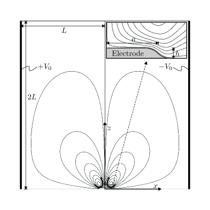
Figure 1: A sketch of the square $2L\times 2L$ electrolytic microchamber in the $xz$-plane. The external voltage $\pm V_{0}$ is applied to the two electrodes (thick black lines) at $x=\pm L$, respectively. It induces two counter-rotating flow rolls (curved black arrows) by electro-osmosis over the un-biased metallic center electrode of length $2a$ and height $h$ placed at the bottom wall around $(x,z)=(0,0)$. The spatial extent of the flow rolls is represented by the streamline plot (thin black curves) drawn as equidistant contours of the flow rate. The inset is a zoom-in on the right half, $0<x<a$, of the un-biased center electrode and the nearby streamlines.

III Full nonlinear model (FN)

We follow the usual continuum approach to the electrokinetic modeling of the electrolytic microchamber and treat only steady-state problems. For simplicity we consider a symmetric, binary electrolyte, where the positive and negative ions with concentrations $c_{+}$ and $c_{-}$, respectively, have the same diffusivity $D$ and charge number $Z$. Using the ideal gas model for the ions, an ion is affected by the sum of an electrical and an osmotic force given by $\bm{F}_{\pm}=\mp Ze\bm{\nabla}\phi-(k_{\mathrm{B}}T/c_{\pm})\>\bm{\nabla}c_{\pm}$. Here $e$ is the elementary charge, $T$ is the absolute temperature and $k_{\textrm{B}}$ is Boltzmann’s constant. Assuming a complete force balance between each ion and the surrounding electrolyte, the resulting body force density $\bm{f}_{\mathrm{ion}}=\sum_{i=\pm}c_{i}\bm{F}_{i}$, appearing in the Navier–Stokes for the electrolyte due to the forces acting on the ions, is

$$\bm{f}_{\mathrm{ion}}=-Ze\big{(}c_{+}-c_{-}\big{)}\bm{\nabla}\phi-k_{\mathrm{B}}T\bm{\nabla}\big{(}c_{+}+c_{-}\big{)}.$$ (3)

As the second term is a gradient, namely the gradient of the osmotic pressure of the ions, it can in the Navier–Stokes equation be absorbed into the pressure gradient $\bm{\nabla}p=\bm{\nabla}p_{\mathrm{dyn}}+\bm{\nabla}p_{\mathrm{os}}$, which is the gradient of the sum of hydrodynamic pressure and the osmotic pressure. Only the electric force is then kept as an explicit body force.

Figure 2: The governing equations (without box) and boundary conditions (with boxes, arrows points to specific boundaries) in dimensionless form (the tilde is omitted for clarity) for the entire quadratic $2L\times 2L$ domain (not shown in correct aspect ratio) bisected into two symmetric halves. Only the right half ($x>0$) of the domain is included in the simulations. The boundaries are the surface of the un-biased center electrode (black rectangle), the solid insulating walls (dark gray lines), the external electrode (black line), and the symmetry line (dashed black line).

III.1 Bulk equations

Neglecting bulk reactions in the electrolyte, the ionic transport is governed by the particle conservation

$$\bm{\nabla}\cdot\bm{J}_{\pm}=0,$$ (4)

where $\bm{J}_{\pm}$ is the flux density of the two ionic species. Assuming the electrolytic solution to be dilute, the ion flux densities are governed by the Nernst–Planck equation

$$\bm{J}_{\pm}=-D\bigg{(}\bm{\nabla}c_{\pm}+\frac{\pm Ze}{k_{\mathrm{B}}T}c_{\pm}\bm{\nabla}\phi\bigg{)}+c_{\pm}\bm{v},$$ (5)

where the first term expresses ionic diffusion and the second term ionic electromigration due to the electrostatic potential $\phi$. The last term expresses the convective transport of ions by the fluid velocity field $\bm{v}$.

The electrostatic potential is determined by the charge density $\rho_{\mathrm{el}}=Ze(c_{+}-c_{-})$ through Poisson’s equation

$$\bm{\nabla}\cdot(\varepsilon\bm{\nabla}\phi)=-\rho_{\mathrm{el}},$$ (6)

where $\varepsilon$ is the fluid permittivity, which is assumed constant. The fluid velocity field $\bm{v}$ and pressure field $p$ are governed the the continuity equation and the Navier–Stokes equation for incompressible fluids,

$$\bm{\nabla}\cdot\bm{v} =0,$$ (7a)

$$\rho_{\textrm{m}}(\bm{v}\cdot\bm{\nabla})\bm{v} =-\bm{\nabla}p+\eta\nabla^{2}\bm{v}-\rho_{\mathrm{el}}\bm{\nabla}\phi,$$ (7b)

where $\rho_{\textrm{m}}$ and $\eta$ are the fluid mass density and viscosity, respectively, both assumed constant.

III.2 Dimensionless form

To simplify the numerical implementation, the governing equations are rewritten in dimensionless form, as summarized in Fig. 2, using the characteristic parameters of the system: The geometric half-length $a$ of the electrode, the ionic concentration $c_{0}$ of the bulk electrolyte, and the thermal voltage $\phi_{0}=k_{\mathrm{B}}T/(Ze)$. The characteristic zeta-potential $\zeta$ of the center electrode, i.e. its induced voltage, is given as the voltage drop along half of the electrode, $\zeta=(a/L)V_{0}$, and we introduce the dimensionless zeta-potential $\alpha$ as $\zeta\equiv\alpha\phi_{0}$, or $\alpha=(aV_{0})/(L\phi_{0})$. The characteristic velocity $u_{0}$ is chosen as the Helmholtz–Smoluchowski slip velocity induced by the local electric field $E=\zeta/a$, and finally the pressure scale is set by the characteristic microfluidic pressure scale $p_{0}=\eta u_{0}/a$. In summary,

$$\phi_{0}=\frac{k_{\mathrm{B}}T}{Ze},\quad u_{0}=\frac{\varepsilon\zeta}{\eta}\frac{\zeta}{a}=\frac{\varepsilon\phi_{0}^{2}}{\eta a}\,\alpha^{2},\quad p_{0}=\frac{\eta u_{0}}{a}.$$ (8)

The new dimensionless variables (denoted by a tilde) thus become

$$\tilde{\bm{r}}=\frac{\bm{r}}{a},\quad\tilde{c}_{i}=\frac{c_{i}}{c_{0}},\quad\tilde{\phi}=\frac{\phi}{\phi_{0}},\quad\tilde{\bm{v}}=\frac{\bm{v}}{u_{0}},\quad\tilde{p}=\frac{p}{p_{0}}.$$ (9)

To exploit the symmetry of the system and the binary electrolyte, the governing equations are reformulated in terms of the average ion concentration $c\equiv(c_{+}+c_{-})/2$ and half the charge density $\rho\equiv(c_{+}-c_{-})/2$. Correspondingly, the average ion flux density $\bm{J}_{c}=(\bm{J}_{+}+\bm{J}_{-})/2$ and half the current density $\bm{J}_{\rho}=(\bm{J}_{+}-\bm{J}_{-})/2$ are introduced. Thus, the resulting full system of coupled nonlinear equations takes the following form for the ionic fields

$$\tilde{\bm{\nabla}}\cdot\tilde{\bm{J}}_{c} =\tilde{\bm{\nabla}}\cdot\tilde{\bm{J}}_{\rho}=0,$$ (10a)

$$\tilde{\bm{J}}_{c} =-\tilde{\rho}\tilde{\bm{\nabla}}\tilde{\phi}-\tilde{\bm{\nabla}}\tilde{c}+\textit{P\'{e}}\>\tilde{c}\tilde{\bm{v}},$$ (10b)

$$\tilde{\bm{J}}_{\rho} =-\tilde{c}\tilde{\bm{\nabla}}\tilde{\phi}-\tilde{\bm{\nabla}}\tilde{\rho}+\textit{P\'{e}}\>\tilde{\rho}\tilde{\bm{v}},$$ (10c)

Pé $$=\frac{u_{0}a}{D},$$ (10d)

while the electric potential obeys

$$\tilde{\bm{\nabla}}^{2}\tilde{\phi}=-\frac{1}{\epsilon^{2}}\tilde{\rho},$$ (11)

and finally the fluid fields satisfy

$$\tilde{\bm{\nabla}}\cdot\tilde{\bm{v}} =0,$$ (12a)

$$\textit{Re}\big{(}\tilde{\bm{v}}\cdot\tilde{\bm{\nabla}}\big{)}\tilde{\bm{v}} =-\tilde{\bm{\nabla}}\tilde{p}+\tilde{\bm{\nabla}}^{2}\tilde{\bm{v}}-\frac{\tilde{\rho}}{\,\epsilon^{2}\,\alpha^{2}}\,\tilde{\bm{\nabla}}\tilde{\phi},$$ (12b)

Re $$=\frac{\rho u_{0}a}{\eta}.$$ (12c)

Here the small dimensionless parameter $\epsilon=\lambda_{\mathrm{D}}/a$ has been introduced, where $\lambda_{\mathrm{D}}$ is the Debye length,

$$\epsilon=\frac{\lambda_{\mathrm{D}}}{a}=\frac{1}{a}\sqrt{\frac{\varepsilon k_{\mathrm{B}}T}{2(Ze)^{2}c_{0}}}.$$ (13)

We note that the dimensionless form of the osmotic force, the second term in Eq. (3), is $\tilde{\bm{f}}^{\mathrm{os}}_{\mathrm{ion}}=-(1/\epsilon^{2}\alpha^{2})\bm{\nabla}\tilde{c}$.

Figure 3: The governing equations (without box) and boundary conditions (with boxes) in dimensionless form (the tilde is omitted) using the logarithmic concentrations (denoted by a breve) of Eq. (18). Otherwise the figure is identical to Fig. 2.

III.3 Boundary conditions

We exploit the symmetry around $x=0$ and consider only the right half ($0<x<L$) of the domain, see Fig. 2. As boundary conditions on the driving electrode we take both ion concentrations to be constant and equal to the bulk charge neutral concentration. Correspondingly, the charge density is set to zero. Consequently, we ignore all dynamics taking place on the driving electrode and simply treat it as an equipotential surface with the value $V_{0}$. We set a no-slip condition for the fluid velocity, and thus at $x=L$ we have

$$\tilde{c}=1,\quad\tilde{\rho}=0,\quad\tilde{\phi}=\frac{V_{0}}{\phi_{0}}=\alpha\frac{L}{a},\quad\tilde{\bm{v}}=\bm{0}.$$ (14)

On the symmetry axis ($x=0$) the potential and the charge density must be zero due to the anti-symmetry of the applied potential. Moreover, there is neither a fluid flux nor a net ion flux in the normal direction and the shear stresses vanish. So at $x=0$ we have

$$\tilde{\phi} =0, \quad\hat{\bm{n}}\cdot\tilde{\bm{J}}_{c} =0, \quad\tilde{\rho} =0,$$ (15a)

$$\hat{\bm{t}}\cdot\tilde{\bm{\sigma}}\cdot\hat{\bm{n}} =0, \hat{\bm{n}}\cdot\tilde{\bm{v}} =0,$$ (15b)

where the stress tensor is $(\bm{\sigma})_{ik}=-p\delta_{ik}+\eta(\partial_{i}u_{k}+\partial_{k}u_{i})$, and $\hat{\bm{n}}$ and $\hat{\bm{t}}$ are the normal and tangential unit vectors, respectively, which in 2D, contrary to 3D, are uniquely defined. The constant potential on the un-biased metallic electrode is zero due to symmetry, and on the electrode surface we apply a no-slip condition on the fluid velocity and no-current condition in the normal direction. So on the electrode surface we have

$$\hat{\bm{n}}\cdot\tilde{\bm{J}}_{c}=0,\quad\hat{\bm{n}}\cdot\tilde{\bm{J}}_{\rho}=0,\quad\tilde{\phi}=0,\quad\tilde{\bm{v}}=\bm{0}.$$ (16)

On the solid, insulating walls there are no fluxes in the normal direction, the normal component of the electric field vanishes and there are no-slip on the fluid velocity.

$$\hat{\bm{n}}\cdot\tilde{\bm{J}}_{c}=0,\quad\hat{\bm{n}}\cdot\tilde{\bm{J}}_{\rho}=0,\quad\hat{\bm{n}}\cdot\bm{\nabla}\tilde{\phi}=0,\quad\tilde{\bm{v}}=\bm{0}.$$ (17)

A complete overview of the governing equations and boundary conditions is given in Fig. 2.

III.4 The strongly nonlinear regime

At high values of the induced $\zeta$-potential, the concentrations of counter- and co-ions acquire very large and very small values, respectively, near the center electrode. Numerically this is problematic. The concentration ratio becomes extremely large and the vanishingly small concentration of co-ions is comparable to the round-off error and may even become negative. However, this numerical problem can be circumvented by working with the logarithms (marked by a breve accent) of the concentration fields, $\breve{c}_{\pm}=\log(c_{\pm}/c_{0})$. By inserting

$$c_{\pm}=c_{0}\,\exp\big{(}\breve{c}_{\pm}\big{)}$$ (18)

in the governing equations (5), (6), and (7b), a new equivalent set of governing equations is derived. The symmetry is exploited by defining the symmetric $\breve{c}=\breve{c}_{+}+\breve{c}_{-}$ and antisymmetric $\breve{\rho}=\breve{c}_{+}-\breve{c}_{-}$ combination of the logarithmic fields and the corresponding formulation of the governing equations is

$$\tilde{\nabla}^{2}\breve{c} =P\acute{e}\,\tilde{\bm{v}}\cdot\tilde{\bm{\nabla}}\breve{c}-\frac{(\tilde{\bm{\nabla}}\breve{c})^{2}\!+\!(\tilde{\bm{\nabla}}\breve{\rho})^{2}}{2}-\tilde{\bm{\nabla}}\tilde{\phi}\cdot\tilde{\bm{\nabla}}\breve{\rho},$$ (19a)

$$\tilde{\nabla}^{2}\big{(}\breve{\rho}+2\tilde{\phi}\big{)} =P\acute{e}\,\tilde{\bm{v}}\cdot\tilde{\bm{\nabla}}\breve{\rho}-\tilde{\bm{\nabla}}\breve{c}\cdot\tilde{\bm{\nabla}}\breve{\rho}-\tilde{\bm{\nabla}}\tilde{\phi}\cdot\tilde{\bm{\nabla}}\breve{\rho},$$ (19b)

$$\tilde{\nabla}^{2}\tilde{\phi} =-\frac{1}{\epsilon^{2}}\,e^{\breve{c}/2}\sinh\left(\frac{\breve{\rho}}{2}\right),$$ (19c)

$$Re\big{(}\tilde{\bm{v}}\cdot\tilde{\bm{\nabla}}\big{)}\tilde{\bm{v}} =-\tilde{\bm{\nabla}}\tilde{p}+\tilde{\nabla}^{2}\tilde{\bm{v}}-\frac{1}{\epsilon^{2}\alpha^{2}}\,e^{\breve{c}/2}\sinh\left(\frac{\breve{\rho}}{2}\right)\tilde{\bm{\nabla}}\tilde{\phi},$$ (19d)

while the continuity equation remains the same as in Eq. (12a). The governing equations and boundary conditions for the logarithmic fields (breve-notation) is summarized in Fig. 3. This transformation serves to help linearize solutions of the dependent variables, $\breve{c}$ and $\breve{\rho}$, at the expense of introducing more nonlinearity into the governing equations.

IV Slip-velocity models

The numerical calculation of ICEO flows in microfluidic systems is generally connected with computational limitations due to the large difference of the inherent length scales. Typically, the Debye length is much smaller than the geometric length scale, $\lambda_{\mathrm{D}}\ll a$, making it difficult to resolve both the dynamics of the Debye layer and the entire microscale geometry with the available computer capacity. Therefore, it is customary to use slip-velocity models, where it is assumed that the electrodes are screened completely by the Debye layer leaving the bulk electrolyte charge neutral. The dynamics of the Debye layer is modeled separately and applied to the bulk fluid velocity through an effective, so-called Helmholtz–Smoluchowski slip velocity condition at the electrode surface,

$$\bm{v}_{\textrm{HS}}=-\frac{\varepsilon}{\eta}\,\zeta\,\bm{E}_{\parallel}.$$ (20)

where $\zeta$ is the zeta potential at the electrode surface, and $\bm{E}_{\parallel}$ is the electric field parallel to the surface. Regardless of the modeled dynamics in the double layer the slip-velocity models are only strictly valid in the limit of infinitely thin double layers $\lambda_{\mathrm{D}}\ll a$.

IV.1 The linear slip-velocity model (LS)

The double-layer screening of the electrodes leaves the bulk electrolyte charge neutral, and hence the governing equations only include the potential $\phi$, the pressure field $p$ and the flow velocity field $\bm{v}$. In dimensionless form they become,

$$\tilde{\bm{\nabla}}^{2}\tilde{\phi} =0,$$ (21a)

$$\textit{Re}\big{(}\tilde{\bm{v}}\cdot\tilde{\bm{\nabla}}\big{)}\tilde{\bm{v}} =-\tilde{\bm{\nabla}}\tilde{p}+\tilde{\bm{\nabla}}^{2}\tilde{\bm{v}},$$ (21b)

$$\tilde{\bm{\nabla}}\cdot\tilde{\bm{v}} =0.$$ (21c)

The electrostatic problem is solved independently of the hydrodynamics, and the potential is used to calculate the effective slip velocity applied to the fluid at the un-biased electrode surface. The boundary conditions of the potential and fluid velocity are equivalent to the conditions applied to the full non-linear system, except at the surface of the un-biased electrode. Here, the normal component of the electric field vanishes, and the effective slip velocity of the fluid is calculated from the electrostatic potential using $\zeta=-\phi$ and $\bm{E}_{\parallel}=-\big{[}(\hat{\bm{t}}\cdot\tilde{\bm{\nabla}})\tilde{\phi}\big{]}\,\hat{\bm{t}}$,

$$\hat{\bm{n}}\cdot\bm{\nabla}\tilde{\phi} =0,$$ (22a)

$$\tilde{\bm{v}}_{\textrm{HS}} =\frac{1}{\alpha^{2}}\,\tilde{\phi}\,\Big{[}(\hat{\bm{t}}\cdot\tilde{\bm{\nabla}})\tilde{\phi}\Big{]}\>\hat{\bm{t}}.$$ (22b)

This represents the simplest possible, so-called linear slip-velocity model; a model which is widely applied as a starting point for numerical simulations of actual microfluidic systems Probstein1994 ; Bruus2008 . In this simple model all the dynamics of the double layer has been neglected, an assumption known to be problematic when the voltage across the electrode exceeds the thermal voltage.

IV.2 The nonlinear slip-velocity model (NLS)

The linear slip-velocity model can be improved by taking into account the nonlinear charge dynamics of the double layer. This is done in the so-called nonlinear slip-velocity model, where, although still treated as being infinitely thin, the double layer has a non-trivial charge dynamics with currents from the bulk in the normal direction and currents flowing tangential to the electrode inside the double layer. For simplicity we assume in the present nonlinear model that the neutral salt concentration $c_{0}$ is uniform. This assumption breaks down at high zeta potentials, where surface transport of ionic species can set up gradients in the salt concentrations leading to chemi-osmotic flow. In future more complete studies of double layer charge dynamics these effects should be included.

The charging of the double layer by the ohmic bulk current is assumed to happen in quasi-equilibrium characterized by a nonlinear differential capacitance $C_{\textrm{dl}}$ given by the Gouy–Chapmann model, $C_{\textrm{dl}}=\varepsilon\cosh[ze\zeta/(2k_{\mathrm{B}}T)]/\lambda_{\mathrm{D}}$, which in the the low-voltage, linear Debye–Hückel regime reduces to $C_{\textrm{dl}}=\varepsilon/\lambda_{\mathrm{D}}$. Ignoring the Stern layer, the zeta-potential is directly proportional to the bulk potential right outside the double layer, $\zeta=-\phi$.

The current along the electrode inside the Debye layer is described by a 2D surface conductance $\sigma_{s}$, which for a binary, symmetric electrolyte is given by Dukhin1993

$$\sigma_{s}=4\lambda_{\mathrm{D}}\sigma(1+m)\sinh^{2}\left(\frac{Ze\zeta}{4k_{\mathrm{B}}T}\right),$$ (23)

where $\sigma$ is the bulk 3D conductivity and

$$m=2\frac{\varepsilon}{\eta D}\left(\frac{k_{\mathrm{B}}T}{Ze}\right)^{2}$$ (24)

is a dimensionless parameter indicating the relative contribution of electroosmosis to surface conduction. In steady state the conservation of charge then yields Soni2009

$$0=\hat{\bm{n}}\cdot(\sigma\bm{\nabla}\phi)+\bm{\nabla}_{s}\cdot\big{[}\sigma_{s}\bm{\nabla}_{s}\phi\big{]},$$ (25)

where the operator $\bm{\nabla}_{s}=\hat{\bm{t}}(\hat{\bm{t}}\cdot\bm{\nabla})$ is the gradient in the tangential direction of the surface.

Given the length scale $a$ of the electrode, the strength of the surface conductance can by characterized by the dimensionless Dukhin number Du defined by

$$Du=\frac{\sigma_{s}}{a\sigma}=\frac{4\lambda_{\mathrm{D}}}{a}(1+m)\sinh^{2}\left(\frac{Ze\zeta}{k_{\mathrm{B}}T}\right).$$ (26)

Conservation of charge then takes the dimensionless form

$$0=\hat{\bm{n}}\cdot(\tilde{\bm{\nabla}}\tilde{\phi})+\tilde{\bm{\nabla}}_{s}\cdot\big{[}Du\tilde{\bm{\nabla}}_{s}\cdot\tilde{\phi}\big{]},$$ (27)

and this effective boundary condition for the potential on the flat electrode constitutes a 1D partial differential equation and as such needs accompanying boundary conditions. As a boundary condition the surface flux is assumed to be zero at the edges of the electrode,

$$\sigma_{s}(\hat{\bm{t}}\cdot\bm{\nabla})\phi\big{|}_{x=\pm a}=0,$$ (28)

which is well suited for the weak formulation we employ in our numerical simulation as seen in Eq. (V).

V Numerics in COMSOL

The numerical calculations are performed using the commercial finite-element-method software COMSOL with second-order Lagrange elements for all the fields except the pressure, for which first-order elements suffices. We have applied the so-called weak formulation mainly to be able to control the coupling between the bulk equations and the boundary constraints, such as Eqs. (22b) and (25), in the implementation of the slip-velocity models in script form.

The Helmholtz–Smoluchowski slip condition poses a numerical challenge because it is a Dirichlet condition including not one, but up to three variables, for which we want a one-directional coupling from the electrostatic field $\phi$ to the hydrodynamic fields $\bm{v}$ and $p$. We use the weak formulation to unambiguously enforce the boundary condition with the explicit introduction of the required hydrodynamic reaction force $\bm{f}$ on the un-biased electrode

$$\bm{f}=\bm{\sigma}\cdot\hat{\bm{n}}.$$ (29)

The $x$ and $z$ components of Navier–Stokes equation are multiplied with test functions $u_{x}$ and $u_{z}$, respectively, and subsequently integrated over the whole domain $\Omega$. Partial integration is then used to move the stress tensor contribution to the boundaries $\partial\Omega$,

$$0=\int_{\partial\Omega}u_{i}\sigma_{ij}n_{j}\textrm{d}s-\int_{\Omega}\big{[}(\partial_{j}u_{i})\sigma_{ij}+u_{i}B_{i}\big{]}\textrm{d}a,$$ (30)

where $B_{i}=Re\left(v_{j}\partial_{j}\right)v_{i}+\rho(\partial_{i}\phi)/(\epsilon^{2}\alpha^{2})$. The boundary integral on the un-biased electrode $\partial\Omega_{\textrm{ue}}$ is rewritten as

$$\int_{\partial\Omega_{\textrm{ue}}}u_{i}\sigma_{ij}n_{j}\textrm{d}s=\int_{\partial\Omega_{\textrm{ue}}}\big{[}u_{i}f_{i}+F_{i}(v_{i}-v_{\textrm{HS},i})\big{]}\textrm{d}s,$$ (31)

where $F_{i}$ are the test functions belonging to the components $f_{i}$ of the reaction force $\bm{f}$. These test functions are used to enforce the Helmholtz–Smoluchowski slip boundary condition consistently. This formulation is used for both slip-velocity models.

In the nonlinear slip-velocity model the Laplace equation (21a) is multiplied with the electrostatic test function $\Phi$ and partially integrated to get a boundary term and a bulk term

$$0=\int_{\partial\Omega}\Phi\left(\partial_{i}\phi\right)n_{i}\textrm{d}s-\int_{\Omega}\left(\partial_{i}\Phi\right)\left(\partial_{i}\phi\right)\textrm{d}a.$$ (32)

The boundary integration term on the electrode is simplified by substitution of Eq. (25) which results in

$$\int_{\partial\Omega_{\textrm{ue}}}\Phi\left(\partial_{i}\phi\right)n_{i}\textrm{d}s=-\int_{\partial\Omega_{\textrm{ue}}}\Phi\left[\hat{t}_{i}\partial_{i}\left(\textit{Du}\,\hat{t}_{j}\partial_{j}\phi\right)\right]\textrm{d}s.$$ (33)

Again, the resulting boundary integral is partially integrated, which gives us explicit access to the end-points of the un-biased electrode. This is necessary for applying the boundary conditions on this 1D electrode,

$$\int_{\partial\Omega_{\textrm{ue}}}\!\!\Phi\Big{[}\hat{t}_{i}\partial_{i}(\textit{Du}\,\hat{t}_{j}\partial_{j}\phi)\Big{]}\textrm{d}s$$

$$\quad=\Big{[}\Phi\textit{Du}\,(\hat{t}_{i}\partial_{i}\phi)\Big{]}_{x=-a}^{x=+a}-\int_{\partial\Omega_{\textrm{ue}}}\!\!(\hat{t}_{i}\partial_{i}\Phi)\textit{Du}\,(\hat{t}_{j}\partial_{j}\phi)\,\textrm{d}s,$$ (34)

The no-flux boundary condition can be explicitly included with this formulation. Note that in both slip-velocity models the zeta-potential is given by the potential just outside the Debye layer, $\zeta=-\phi$, and it is therefore not necessary to include it as a separate variable.

The accuracy and the mesh dependence of the simulation as been investigated as follows. The comparison between the three models quantifies relative differences of orders down to $10^{-3}$, and the convergence of the numerical results is ensured in the following way. COMSOL has a build-in adaptive mesh generation technique that is able to refine a given mesh so as to minimize the error in the solution. The adaptive mesh generator increases the mesh density in the immediate region around the electrode to capture the dynamics of the ICEO in the most optimal way under the constraint of a maximum number of degrees of freedom (DOFs). For a given set of physical parameters, the problem is solved each time increasing the number of DOFs and comparing consecutive solutions. As a convergence criterium we demand that the standard deviation of the kinetic energy relative to the mean value should be less than a given threshold value typically chosen to be around $10^{-5}$. All of the simulations ended with more than $10^{6}$ DOFs, and the ICEO flow is therefore sufficiently resolved even for the thinnest double layers in our study for which $\epsilon=10^{-4}$.

VI Results

Our comparison of the three numerical models is primarily focused on variations of the three dimensionless parameters $\epsilon$, $\alpha$, and $\beta$ relating to the Debye length $\lambda_{\mathrm{D}}$, the applied voltage $V_{0}$, and the height $h$ of the electrode, respectively,

$$\epsilon=\frac{\lambda_{\mathrm{D}}}{a},\quad\alpha=\frac{aV_{0}}{L\phi_{0}},\quad\beta=\frac{h}{a}.$$ (35)

As mentioned in Sec. I, the strength of the generated ICEO flow can be measured as the mechanical power input $P_{\mathrm{mech}}$ exerted on the electrolyte by the slip-velocity just outside the Debye layer or equivalently by the kinetic energy dissipation $P_{\mathrm{kin}}$ in the bulk of the electrolyte. However, both these methods suffers from numerical inaccuracies due to the dependence of both the position of the integration path and of the less accurately determined velocity gradients in the stress tensor $\bm{\sigma}$. To obtain a numerically more stable and accurate measure, we have chosen in the following analysis to characterize the strength of the ICEO flow by the kinetic energy $E_{\mathrm{kin}}$ of the induced flow field $\bm{v}$,

$$E_{\mathrm{kin}}=\mbox{$\frac{1}{2}$}\rho_{\textrm{m}}\int_{\Omega}\!v^{2}\>\mathrm{d}x\,\mathrm{d}z,$$ (36)

which depends on the velocity field and not its gradients, and which furthermore is a bulk integral of good numerical stability.

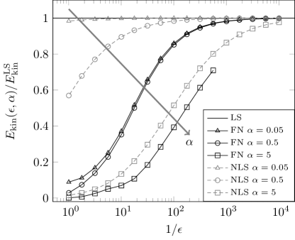
Figure 4: The total induced kinetic energy $E^{\mathrm{NLS}}_{\mathrm{kin}}$ (gray dashed) and $E^{\mathrm{FN}}_{\mathrm{kin}}$ (black) for the nonlinear slip-velocity model and the full model, respectively, relative to $E^{\mathrm{LS}}_{\mathrm{kin}}$ (horizontal black line) of the linear slip-velocity model as a function of dimensionless inverse Debye length $1/\epsilon$. Each are shown for three values of the dimensionless applied voltage $\alpha=0.05,0.5$ and 5. The value of $\epsilon$ decreases from 1 to $10^{-4}$ going from left to right.

VI.1 Zero height of the un-biased center electrode

We assume the height $h$ of the un-biased center electrode to be zero, i.e. $\beta=0$, while varying the Debye length and the applied voltage through the parameters $\epsilon$ and $\alpha$. We note that the linear slip-velocity model Eqs. (21) and (22) is independent of the dimensionless Debye length $\epsilon$. It is therefore natural to use the kinetic energy $E^{\mathrm{LS}}_{\mathrm{kin}}$ of this model as a normalization factor.

In the lin-log plot of Fig. 4 we show the kinetic energy $E^{\mathrm{NLS}}_{\mathrm{kin}}$ and $E^{\mathrm{FN}}_{\mathrm{kin}}$ normalized by $E^{\mathrm{LS}}_{\mathrm{kin}}$ as a function of the inverse Debye length $1/\epsilon$ for three different values of the applied voltage, $\alpha=0.05,0.5$ and 5, ranging from the linear to the strongly nonlinear voltage regime.

We first note that in the limit of vanishing Debye length (to the right in the graph) all models converge towards the same value for all values of the applied voltage $\alpha$. For small values of $\alpha$ the advanced slip-velocity model $E^{\mathrm{NLS}}_{\mathrm{kin}}$ is fairly close to the linear slip-velocity model $E^{\mathrm{LS}}_{\mathrm{kin}}$, but as $\alpha$ increases, it requires smaller and smaller values of $\epsilon$ to obtain the same results in the two models. In the linear regime $\alpha=0.05$ a deviation less than 5% is obtained already for $\epsilon<1$. In the nonlinear regime $\alpha=0.5$ the same deviation requires $\epsilon<10^{-2}$, while in the strongly nonlinear regime $\epsilon<10^{-4}$ is needed to obtain a deviation lower than 5%.

In contrast, it is noted how the more realistic full model $E^{\mathrm{FN}}_{\mathrm{kin}}$ deviates strongly from $E^{\mathrm{LS}}_{\mathrm{kin}}$ for most of the displayed values of $\epsilon$ and $\alpha$. To obtain a relative deviation less than 5% in the linear ($\alpha=0.05$) and nonlinear ($\alpha=0.5$) regimes, a minute Debye length of $\epsilon<10^{-3}$ is required, and in the strongly nonlinear regime the 5% level it not reached at all.

The deviations are surprisingly large. The Debye length in typical electrokinetic experiments is $\lambda_{\mathrm{D}}=30$ nm. For a value of $\epsilon=0.01$ this corresponds to an electrode of width $2\times 3~{}\textrm{\textmu{}m}=6~{}\textrm{\textmu{}m}$, comparable to those used in Refs. Studer2004 ; Cahill2004 ; Gregersen2007 . In Fig. 4 we see that for $\alpha=5$, corresponding to a moderate voltage drop of 0.26 V across the electrode, the linear slip-velocity model overestimates the ICEO strength by a factor 1/0.4 = 2.5. The nonlinear slip-model does a better job. For the same parameters it only overestimates the ICEO strength by a factor 0.5/0.4 = 1.2.

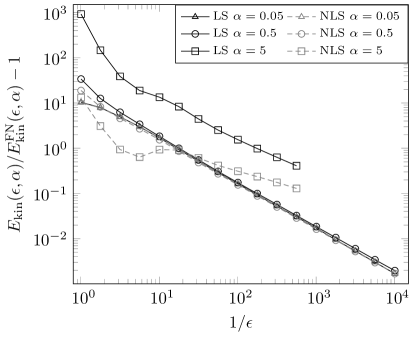
Figure 5: The difference between the induced kinetic energies $E^{\mathrm{LS}}_{\mathrm{kin}}$ and $E^{\mathrm{NLS}}_{\mathrm{kin}}$ of the linear and nonlinear slip-velocity models, respectively, relative to the full model $E^{\mathrm{FN}}_{\mathrm{kin}}$ as a function of the inverse Debye length $1/\epsilon$. for three different applied voltages $\alpha=0.05,0.5,5$.

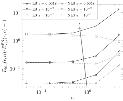
Figure 6: The difference between the induced kinetic energies $E^{\mathrm{LS}}_{\mathrm{kin}}$ and $E^{\mathrm{NLS}}_{\mathrm{kin}}$ of the linear and nonlinear slip-velocity models, respectively, relative to the full model $E^{\mathrm{FN}}_{\mathrm{kin}}$ as a function of the voltage bias $\alpha$ for three different Debye layer thicknesses $\epsilon=1.8\times 10^{-3},10^{-2},10^{-1}$.

For more detailed comparisons between the three models the data of Fig. 4 are plotted in a different way in Fig. 5. Here the overestimates $(E^{\mathrm{LS}}_{\mathrm{kin}}/E^{\mathrm{FN}}_{\mathrm{kin}})-1$ and $(E^{\mathrm{NLS}}_{\mathrm{kin}}/E^{\mathrm{FN}}_{\mathrm{kin}})-1$ of the two slip-velocity models relative to the more correct full model are plotted in a log-log plot as a function of the inverse Debye length $1/\epsilon$ for three different values of the applied voltage. It is clearly seen how the relative deviation decreases proportional to $\epsilon$ as $\epsilon$ approaches zero.

Finally, in Fig. 6 the relative deviations $(E^{\mathrm{LS}}_{\mathrm{kin}}/E^{\mathrm{FN}}_{\mathrm{kin}})-1$ and $(E^{\mathrm{NLS}}_{\mathrm{kin}}/E^{\mathrm{FN}}_{\mathrm{kin}})-1$ are plotted versus the voltage $\alpha$ in a log-log plot. For any value of the applied voltage $\alpha$, both slip-velocity models overestimates by more than 100% for large Debye lengths $\epsilon=10^{-1}$ and by more than 10% for $\epsilon=10^{-2}$. For the minute Debye length $\lambda_{\mathrm{D}}=1.8\times 10^{-3}$ the overestimates are about 3% in the linear and weakly nonlinear regime $\alpha<1$, however, as we enter the strongly nonlinear regime with $\alpha=5$ the overestimation increases to a level above 10%.

VI.2 Finite height of the un-biased electrode

Compared to the full numerical model, the slip-velocity models are convenient to use, but even for small Debye lengths, say $\lambda_{\mathrm{D}}=0.01a$, they are prone to significant quantitative errors as shown above. Similarly, it is of relevance to study how the height of the un-biased electrode influences the strength of the ICEO flow rolls. In experiments the thinnest electrodes are made by evaporation techniques. The resulting electrode heights are of the order 50 nm $-$ 200 nm, which relative to the typical electrode widths $a\approx 5~{}\textrm{\textmu{}m}$ results in dimensionless heights $10^{-3}<\beta<10^{-1}$.

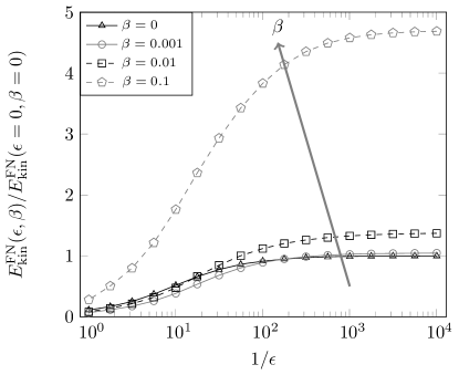
Figure 7: The difference between the induced kinetic energies $E^{\mathrm{FN}}_{\mathrm{kin}}(\epsilon,\beta)$ of the full model at finite Debye length and electrode height relative to the full model $E^{\mathrm{FN}}_{\mathrm{kin}}(0,0)$ at zero Debye length and zero electrode height as a function of the inverse Debye length $1/\epsilon$ for four electrode heights $\beta=0,10^{-3},10^{-2},10^{-1}$.

In Fig. 7 is shown the results for the numerical calculation of the kinetic energy $E^{\mathrm{FN}}_{\mathrm{kin}}(\epsilon,\beta)$ using the full numerical model. The dependence on the kinetic energy of the dimensionless Debye length $\epsilon=\lambda_{\mathrm{D}}/a$ and the dimensionless electrode height $\beta=h/a$ is measured relative to the value $E^{\mathrm{FN}}_{\mathrm{kin}}(\epsilon,\beta)$ of the infinitely small Debye length for an electrode of zero height. For small values of the height no major deviations are seen. The curve for $\beta=0$ and $\beta=0.001$ are close. As the height is increased to $\beta=10^{-2}$ we note that the strength of the ICEO is increased by 20%$-$25% as $\beta>\epsilon$. This tendency is even stronger pronounced for the higher electrode $\beta=10^{-1}$. Here the ICEO strength is increased by approximately 400% for a large range of Debye lengths.

VI.3 Thermodynamic efficiency of the ICEO system

Conventional electro-osmosis is known to have a low thermodynamic efficiency defined as the delivered mechanical pumping power relative to the total power delivered by the driving voltage. Typical efficiencies are of the order of 1% Laser2004 , while in special cases an efficiency of 5.6% have been reported Reichmuth2003 . In the following we provide estimates and numerical calculations of the corresponding thermodynamic efficiency of the ICEO system.

The applied voltage drop $2V_{0}=2E_{0}L$ across the system in the $x$-direction is written as the average electrical field $E_{0}$ times the length $2L$, while the electrical current is given by $I=WH\sigma E_{0}$, where $W$ and $H$ is the width and height in the $y$- and $z$-direction, respectively, and $\sigma=D\varepsilon/\lambda_{\mathrm{D}}^{2}=\varepsilon/\tau_{D}$ is the conductivity written in terms of the Debye time $\tau_{D}=\lambda_{\mathrm{D}}^{2}/D$. The total power consumption to run the ICEO system is thus

$$P_{\mathrm{tot}}=2V_{0}\times I=\frac{4}{\tau_{\mathrm{D}}}\>\Big{(}\frac{1}{2}\varepsilon E_{0}^{2}\Big{)}LWH.$$ (37)

This expression can be interpreted as the total energy, $\frac{1}{2}\varepsilon E_{0}^{2}\times LWH$, stored in the average electrical field of the system with volume $LWH$ multiplied by the characteristic electrokinetic rate $4/\tau_{\mathrm{D}}$.

The velocity-gradient part of the hydrodynamic stress tensor is denoted $\tilde{\bm{\sigma}}$, i.e. $(\tilde{\bm{\sigma}})_{ij}=\eta(\partial_{i}v_{j}+\partial_{j}v_{i})$. In terms of $\tilde{\bm{\sigma}}$, the kinetic energy dissipation $P_{\mathrm{kin}}$ necessary to sustain the steady-state flow rolls is given by $P_{\mathrm{kin}}=\frac{W}{2\eta}\int_{0}^{L}\mathrm{d}x\>\int_{0}^{H}\mathrm{d}z\>\mathrm{Tr}(\tilde{\bm{\sigma}}^{2})$. In the following estimate we work in the Debye–Hückel limit for an electrode of length $2a$, where the induced zeta potential is given by $\zeta_{\mathrm{ind}}=aE_{0}$ and the radius of each flow roll is approximately $a$. In this limit the electro-osmotic slip velocity $u_{\mathrm{eo}}$ and the typical size of the velocity gradient $|\partial_{i}v_{j}|$ are

$$u_{\mathrm{eo}} =\frac{\varepsilon\zeta_{\mathrm{ind}}}{\eta}\>E_{0}=\frac{\varepsilon a}{\eta}\>E_{0}^{2},$$ (38a)

$$|\partial_{i}v_{j}| \approx\frac{u_{\mathrm{eo}}}{a}=\frac{\varepsilon}{\eta}\>E_{0}^{2}.$$ (38b)

Thus, since the typical area covered by each flow roll is $\pi a^{2}$ , we obtain the following estimate of $P_{\mathrm{kin}}$,

$$P_{\mathrm{kin}}\approx 2\frac{W}{2\eta}\>\pi a^{2}\>4\bigg{[}\eta\frac{u_{\mathrm{eo}}}{a}\bigg{]}^{2}=8\>\frac{\varepsilon E_{0}^{2}}{\eta}\>\Big{(}\frac{1}{2}\varepsilon E_{0}\Big{)}^{2}\pi a^{2}W.$$ (39)

Here the power dissipation can be interpreted as the energy of the electrical field in the volume $\pi a^{2}W$ occupied by each flow roll multiplied by an ICEO rate given by the electric energy density $\varepsilon E_{0}^{2}$ divided by the rate of viscous energy dissipation per volume given by $\eta$.

The thermodynamic efficiency can now be calculated as the ratio $P_{\mathrm{kin}}/P_{\mathrm{tot}}$ using Eqs. (37) and (39),

$$\frac{P_{\mathrm{kin}}}{P_{\mathrm{tot}}}\approx\frac{2\pi a^{2}}{LH}\>\frac{\varepsilon E_{0}^{2}}{\eta/\tau_{\mathrm{D}}}\approx 2.4\times 10^{-8}.$$ (40)

This efficiency is the product of the ratio between the volumes of the flow rolls and the entire volume multiplied and the ratio of the electric energy density in the viscous energy density $\eta/\tau_{\mathrm{D}}$. The value is found using $L=H=15a=0.15$ mm, $E_{0}=2.5$ kV/m, and $\lambda_{\mathrm{D}}=20$ nm, which is in agreement with the conventional efficiencies for conventional electro-osmotic systems quoted above.

VII Conclusion

We have shown that the ICEO velocities calculated using the simple zero-width models significantly overestimates those calculated in more realistic models taking the finite size of the Debye screening length into account. This may provide a partial explanation of the observed quantitative discrepancy between observed and calculated ICEO velocities. The discrepancy increases substantially for increasing $\epsilon$, i.e. in nanofluidic systems.

Even larger deviations of the ICEO strength is calculated in the full numerical model when a small, but finite height of the un-biased electrode is taken into account.

A partial explanation of the quantitative failure of the analytical slip velocity model is the decrease of the tangential electric field as a function of the distance to the surface of the polarized ICEO object combined with the spatial extent of the charge density of the double layer. Also tangential hydrodynamic and osmotic pressure gradients developing inside the double layer may contribute to the lowering ICEO strength when taking the finite width of the double layer into account. The latter may be related to the modification of the classical Helmholtz–Smoluchowski expression of the slip-velocity obtained by adding a term proportional to the gradient of the salt concentration $c$ Khair2008b .

Our work shows that for systems with a small, but non-zero Debye length of 0.001 to 0.01 times the size of the electrode, and even when the Debye-Hückel approximation is valid, a poor quantitative agreement between experiments and model calculations must be expected when applying the linear slip-velocity model based on a zero Debye-length. It is advised to employ the full numerical model of ICEO, when comparing simulations with experiments.

VIII Acknowledgements

We thank Sumita Pennathur and Martin Bazant for illuminating discussions, and we are particularly grateful to Todd Squires for a number of valuable comments and suggestions. This work is supported in part by the Institute for Collaborative Biotechnologies through contract no. W911NF-09-D-0001 from the U.S. Army Research Office. The content of the information herein does not necessarily reflect the position or policy of the Government and no official endorsement should be inferred.

References

- (1) S.S. Dukhin, Adv. Colloid Interface Sci. 44, 1 (1993).
- (2) V.A. Murtsovkin, Colloid J. 58, 341 (1996).
- (3) A. Gonzalez, A. Ramos, N.G. Green, A. Castellanos and H. Morgan, Phys. Rev. E 61(4), 4019 (2000).
- (4) N.G. Green, A. Ramos, A. Gonzalez, H. Morgan and A. Castellanos, Phys. Rev. E 66, 026305 (2002).
- (5) A. Ajdari, Phys. Rev. E 61, R45 (2000).
- (6) A.B.D. Brown, C.G. Smith and A.R. Rennie, Phys. Rev. E 63, 016305 (2000).
- (7) V. Studer, A. Pépin, Y. Chen and A. Ajdari, The Analyst 129, 944 (2004).
- (8) D. Lastochkin, R. Zhou, P. Whang, Y. Ben and H.-C. Chang, J. Appl. Phys. 96, 1730 (2004).
- (9) S. Debesset, C.J. Hayden, C. Dalton, J.C.T. Eijkel and A. Manz, Lab Chip 4, 396 (2004).
- (10) B.P. Cahill, L.J. Heyderman, J. Gobrecht and A. Stemmer, Phys. Rev. E 70, 036305 (2004).
- (11) M.M. Gregersen, L.H. Olesen, A. Brask, M.F. Hansen, and H. Bruus, Phys. Rev. E 76 056305 (2007).
- (12) L.H. Olesen, H. Bruus and A. Ajdari, Phys. Rev. E 73, 056313 (2006).
- (13) T.M. Squires, and M.Z. Bazant, J. Fluid Mech. 509, 217 (2004).
- (14) J.A. Levitan, S. Devasenathipathy, V. Studer, Y. Ben, T. Thorsen, T.M. Squires, and M.Z. Bazant, Coll. Surf. A 267, 122 (2005).
- (15) T.M. Squires, and M.Z. Bazant, J. Fluid Mech. 560, 65 (2006).
- (16) C.K. Harnett, J. Templeton, K. Dunphy-Guzman, Y.M. Senousy, and M.P. Kanouff, Lab Chip 8, 565 (2008).
- (17) A.S. Khair and T.M. Squires, J. Fluid Mech. 615, 323 (2008).
-
(18)
M.M. Gregersen, F. Okkels, M.Z. Bazant, and H. Bruus,
New J. Phys. (submitted, 2008),
http://arxiv.org/abs/0901.1788 - (19) G. Soni, T.M. Squires, and C.D. Meinhart, in Proceedings of 2007 ASME International Mechanical Engineering Congress and Exposition, 2007.
- (20) R.F. Probstein, Physicochemical hydrodynamics, (John Wiley & Sons, New York, 1994).
- (21) H. Bruus, Theoretical Microfluidics, (Oxford University Press, Oxford, 2008).
- (22) S.S. Dukhin, R. Zimmermann, and C. Werner, Coll. Surf. A 195, 103 (2001).
- (23) J. Lyklema, J. Phys.: Condens. Matter 13, 5027 (2001).
- (24) K.T. Chu, and M.Z. Bazant, J. Colloid. Interf. Sci. 315, 319 (2007).
- (25) G. Soni, M.B. Andersen, H. Bruus, T. Squires, C. Meinhart, Phys. Rev. E (in preparation, 2009)
- (26) D.J. Laser and J.G. Santiago J. Micromech. Microeng. 14, R1 (2004).
- (27) D.S. Reichmuth, G.S. Chirica, and B.J. Kirby Sens. Actuators B 92, 37 (2003).
- (28) A.S. Khair and T.M. Squires, Phys. Fluids 20, 087102 (2008)