Can TiO Explain Thermal Inversions in the Upper Atmospheres of Irradiated Giant Planets?

Abstract

Spitzer Space Telescope infrared observations indicate that several transiting extrasolar giant planets have thermal inversions in their upper atmospheres. Above a relative minimum, the temperature appears to increase with altitude. Such an inversion probably requires a species at high altitude that absorbs a significant amount of incident optical/UV radiation. Some authors have suggested that the strong optical absorbers titanium oxide (TiO) and vanadium oxide (VO) could provide the needed additional opacity, but if regions of the atmosphere are cold enough for Ti and V to be sequestered into solids they might rain out and be severely depleted. With a model of the vertical distribution of a refractory species in gaseous and condensed form, we address the question of whether enough TiO (or VO) could survive aloft in an irradiated planet’s atmosphere to produce a thermal inversion. We find that it is unlikely that VO could play a critical role in producing thermal inversions. Furthermore, we find that macroscopic mixing is essential to the TiO hypothesis; without macroscopic mixing, such a heavy species cannot persist in a planet’s upper atmosphere. The amount of macroscopic mixing that is required depends on the size of condensed titanium-bearing particles that form in regions of an atmosphere that are too cold for gaseous TiO to exist. We parameterize the macroscopic mixing with the eddy diffusion coefficient $K_{zz}$ and find, as a function of particle size $a$, the values that $K_{zz}$ must assume on the highly irradiated planets HD 209458b, HD 149026b, TrES-4, and OGLE-TR-56b to loft enough titanium to the upper atmosphere for the TiO hypothesis to be correct. On these planets, we find that for TiO to be responsible for thermal inversions $K_{zz}$ must be at least a few times $10^{7}\rm~{}cm^{2}~{}s^{-1}$, even for $a=0.1~{}\mu$m, and increases to nearly $10^{11}\rm~{}cm^{2}~{}s^{-1}$ for $a=10~{}\mu$m. Such large values may be problematic for the TiO hypothesis, but are not impossible.

1 Introduction

In the last two decades, we have moved from the first discoveries of planets beyond our solar system (Wolszczan & Frail, 1992; Mayor & Queloz, 1995; Marcy & Butler, 1996) to having the ability to frame and address questions about the structures of distant worlds. The remarkable pace of detections has accelerated to the point that there are now more than $\sim$340 extrasolar planets currently known, of which more than 55 transit their primaries.

The transiting planets, first discovered by Henry et al. (2000) and Charbonneau et al. (2000), constitute a particularly exciting subsample. Knowing that their orbits are edge-on breaks the degeneracy between their masses and orbital inclination angles. Furthermore, their atmospheres may be probed during both primary eclipse (Seager & Sasselov, 2000; Hubbard et al., 2001; Brown, 2001) and secondary eclipse (Sudarsky et al., 2000, 2003; Rauscher et al., 2007; Burrows et al., 2008; Fortney et al., 2008).

Early speculative calculations are now supplemented with a wealth of observational data that constrain the atmospheres of several transiting extrasolar giant planets (EGPs). The strong doublets at $\sim$5900 Å and $\sim$7700 Å in neutral sodium (Na) and potassium (K) contribute significantly to the opacity of planetary atmospheres through much of the optical range. The sodium feature has been seen in the transit spectra of both HD 209458b (Charbonneau et al., 2002; Désert et al., 2008) and HD 189733b (Redfield et al., 2008). Charbonneau et al. (2002) point out that the depth of the observed Na feature is less than would be expected if neutral sodium were present at solar abundance. Iro et al. (2005) suggest that if, as expected, HD 209458b is in synchronous rotation, then Na might have condensed into Na₂S on the colder night side, which could in part explain an inferred low abundance of atomic Na. Another possible explanation is a high gray haze (Charbonneau et al., 2002; Fortney et al., 2003).

In the simplest picture of an atmosphere’s vertical thermal profile, temperature decreases with altitude (with decreasing pressure). In certain cases of high stellar irradiation, however, a chemical species that is a strong optical or near UV absorber could, if present at high altitude, lead to a thermal inversion in which the temperature increases above a relative minimum (Hubeny et al., 2003). Such an inversion is well-known in the context of the Earth’s stratosphere (Sherwood & Dessler, 2001), where the upper-atmosphere heating is caused mainly by UV absorption by ozone. Infrared observations by the Spitzer Space Telescope have suggested that several giant planets have such thermal inversions, including HD 209458b (Burrows et al., 2007b; Knutson et al., 2008a), HD 149026b (Fortney et al., 2006; Burrows et al., 2008), TrES-4 (Knutson et al., 2009), XO-1b (Machalek et al., 2008), and, perhaps, $\upsilon$ Andromeda b (Burrows et al., 2008). It is not known, however, what species is responsible for the additional opacity high in these planets’ atmospheres.

Titanium (Ti) and vanadium (V) both play significant roles in the spectra of low-mass stellar objects, such as M-dwarfs (Kirkpatrick et al., 1999; Martín et al., 1999; Lodders, 2002). Their oxides (TiO and VO) in gaseous form are strong optical absorbers that, if present at near-solar abundance in the upper atmospheres of highly irradiated planets, could cause thermal inversions (Hubeny et al., 2003; Fortney et al., 2006, 2008; Burrows et al., 2008). It might be difficult, though, to maintain significant quantities of gaseous TiO/VO aloft. First, TiO and VO are significantly heavier than the primary constituent of EGP atmospheres, molecular hydrogen. In the battle of molecular diffusion against gravitational settling, heavier molecules settle more strongly and are concentrated at deep layers. Macroscopic mixing processes, such as turbulent diffusion or large-scale advective motions, are then required to maintain a high abundance of a heavy species at altitude.

Second, and perhaps more significant, Ti and V might rain out of the upper atmospheres. In chemical equilibrium, at low temperatures or high pressures, Ti and V are found in a variety of condensates that form solid grains (Burrows & Sharp, 1999; Lodders, 2002; Sharp & Burrows, 2007). Radiative equilibrium radiative transfer models of close-in EGP atmospheres (Sudarsky et al., 2003; Hubeny et al., 2003; Burrows et al., 2007a; Fortney et al., 2006, 2008) predict that, in at least some of the planets inferred to have inversions (e.g., HD 209458b), there is a cooler region below the inversion in which the temperature and pressure would cause Ti and V to be in their condensed, solid phases. Such a region may aptly be called a “cold-trap,” in analogy with the Earth’s equatorial water cold-trap. Above the Earth’s equator, the atmosphere cools and reaches a relative minimum at the tropopause, the beginning of the stratospheric thermal inversion. As a result, even though water could exist in gaseous form at altitude, most water condenses and rains out before ever reaching the stratosphere, leaving the stratosphere quite dry (Brewer, 1949; Sherwood & Dessler, 2001). If a similar rain-out process occurs in the Ti/V cold-traps of giant planets, their upper atmospheres could be similarly depleted of TiO and VO.

Furthermore, there could be other cold-traps. Short-period EGPs are generally presumed to be tidally locked in synchronous rotation (Goldreich & Peale, 1966; Spiegel et al., 2007). The large contrast between the intense stellar forcing at the substellar point and the minimal heating at the poles and on the night sides of synchronously rotating planets can lead to large temperature differences and powerful winds, as has been predicted by atmospheric general circulation models (GCMs) (Showman & Guillot, 2002; Cho et al., 2003; Menou et al., 2003; Cooper & Showman, 2005; Burkert et al., 2005; Langton & Laughlin, 2007, 2008b, 2008a; Cho et al., 2008; Dobbs-Dixon & Lin, 2008; Showman et al., 2008a; Dobbs-Dixon, 2008; Menou & Rauscher, 2008; Showman et al., 2008b). Transport of gaseous TiO/VO to the night side of a planet by zonal winds could lead to the condensation and settling out of these odixes, as considered by Showman et al. (2008b). Though settling might be slow on orbital timescales (depending on condensate size), if the night side remains a sink for hundreds of millions of years or more it could inevitably lead to significant depletion of a planet’s upper atmosphere.

The same types of mixing processes that might loft heavy molecules to greater altitudes than could molecular diffusion might also help loft grains or droplets. If turbulent mixing on a macroscopic scale is vigorous enough, the condensates of Ti/V in the cold-trap could be stirred up into the hot, more rarified upper atmosphere, where they might reform their optically important oxides.

Nevertheless, recent observational evidence suggests that the upper atmosphere of HD 209458b might indeed be deficient in TiO. Désert et al. (2008) find that, redward of the Na D lines, the near-constancy of the planet’s transit radius places a limit on the TiO abundance of $\sim$10${}^{-2}-10^{-3}$ solar, an amount that, as we show in §2, is insufficient to explain the inferred thermal inversion. This observation is not proof that TiO is underabundant in the upper atmosphere of HD 209458b, because transit spectroscopy probes only atmospheric regions near the terminator. It is conceivable that the terminator is depleted of TiO, but the substellar point is not.

To address this issue, this paper introduces a model for the abundances of TiO and VO in the upper atmospheres of highly irradiated EGPs. We conclude that VO does not contribute significantly to thermal inversions. We use our model to estimate the minimum amount of macroscopic mixing that would be necessary to make the TiO hypothesis viable on several highly-irradiated planets. We find that for HD 209458b, HD 149026b, TrES-4, OGLE-TR-56b, and WASP-12b, significant macroscopic mixing would be necessary, an amount that it is not at all clear actually obtains. Our model predicts that, for TiO to be present in the upper atmosphere at sufficient quantity to cause thermal inversion, $K_{zz}$ must be at least a few times $10^{7}\rm~{}cm^{2}~{}s^{-1}$ for 0.1-$\mu$m particles, increasing roughly linearly with condensate particle size. HD 209458b has the most severe cold trap of the planets we considered. There, for particles from 0.1 $\mu$m to 10 $\mu$m in radius, $K_{zz}$ must be nearly $\sim$10${}^{9}\rm~{}cm^{2}~{}s^{-1}$ to nearly $\sim$10${}^{11}\rm~{}cm^{2}~{}s^{-1}$, respectively. For larger particles, even greater values of $K_{zz}$ would be required. WASP-12b has no day-side cold trap in our models; there, we find that $K_{zz}$ must be $\sim$$2\times 10^{7}\rm~{}cm^{2}~{}s^{-1}$.

The remainder of this paper is structured as follows: In §2, we present the model. We describe how we generate temperature-pressure profiles and spectra of irradiated expolanets, and we parameterize the upper atmosphere abundance of a condensing species in the presence of turbulent and molecular diffusion. Section 3 contains the results of our calculations, and §4 discusses a few remaining complications. Finally, in §5, we summarize our findings.

2 Modeling the Vertical Distribution of Condensates

Atmospheres mix their constituents in a variety of ways, at a range of different spatial scales. At the micro-level, molecular diffusion operates; at the macro-level, turbulent mixing and large-scale advective motions that (including planetary-scale winds) are likely to be dominant. How much TiO would have to be mixed through these various processes, up to the low pressures of the upper atmosphere of an EGP, in order to cause a thermal inversion? To address this question, in § 2.1 we produce one-dimensional radiative transfer atmosphere models. We then, in § 2.2, examine how titanium condensates are likely to be distributed within these atmosphere models and, therefore, how much gaseous TiO is actually likely to reach the high parts of the atmosphere, where it would have to be if it indeed is the needed extra absorber.

2.1 The Radiative Model

To generate temperature-pressure profiles and spectra for the day and night sides of several EGPs, we compute model atmospheres with the code COOLTLUSTY, described in Hubeny et al. (2003), Sudarsky et al. (2003), Burrows et al. (2006), and Burrows et al. (2008). This code is an offshoot of the code TLUSTY (Hubeny, 1988; Hubeny & Lanz, 1995), with chemical abundances and molecular opacities appropriate to the (relatively) cooler environments of planetary atmospheres and brown dwarfs (Sharp & Burrows, 2007; Burrows & Sharp, 1999; Burrows et al., 2001). Irradiation in planetary atmosphere models is incorporated using Kurucz model stellar spectra, interpolated to temperatures and surface gravities appropriate to exoplanet host stars (Kurucz, 1979, 1994, 2005).

In most of our radiative transfer model calculations, we assume gaseous TiO or VO throughout the entire atmosphere. We note that analysis based on this assumption is not strictly self-consistent, because we use the $T$-$P$ profiles generated from this assumption to calculate where in fact these gaseous species exist. Nonetheless, because our models indicate that gaseous TiO and VO have most of their radiative influence high in a planet’s atmosphere, the model condition that these species are present in cold-trap regions serves mainly to avoid discontinuities in opacity versus depth and, therefore, to aid convergence of the models. This procedure should not introduce large errors.

Burrows et al. (2006) propose a formalism for treating the redistribution of incident stellar flux in a planet’s atmosphere in which the proportion of day-side bolometric stellar flux that is transported to, and reradiated from, the night side is $P_{n}$. This redistribution parameter plausibly ranges between 0, corresponding to all stellar flux being instantaneously reradiated, and 0.5, corresponding to the night side receiving exactly as much stellar energy as the day side (as a result of advective heat redistribution). Burrows et al. (2008) suggest that in many situations $P_{n}$ is likely to vary between 0.1 and 0.4. In this study, we take $P_{n}=0.3$, and apply the redistribution between 0.01 and 0.1 bars, for all models.

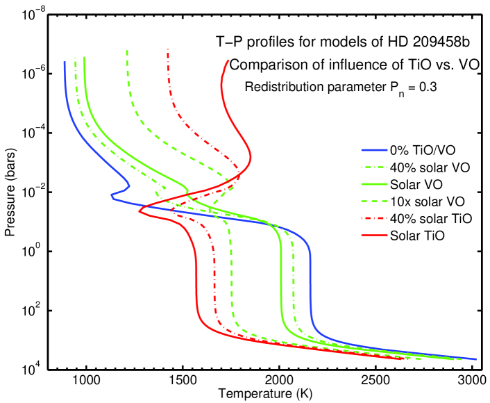
Figure 1: Comparison of the influence of TiO and VO. Temperature-pressure profiles for six models of HD 209458b are presented, one with no TiO or VO (blue), three with different mixing ratios of VO, but not TiO (green), and two with TiO, but not VO. Even 10 times solar abundance of VO has less of an influence on the profile than just 40% solar TiO. This suggests that it is unlikely that VO plays an important role in determining whether a highly irradiated EGP has a thermal inversion. The dimple at $\sim$10^-2 bars in the profile for the model with no TiO/VO is caused by the redistribution to the night side, parameterized by $P_{n}=0.3$ (Burrows et al., 2006).

First, we note that it is unlikely that VO plays a crucial determining role in an EGP’s atmospheric structure. Titanium and vanadium are both trace elements, but Ti is about $\sim$10 times as abundant as V: Ti’s solar abundance relative to hydrogen is $\sim 10^{-7}$, whereas V’s is $\sim 10^{-8}$ (Anders & Grevesse, 1989). Furthermore, TiO’s optical opacity is generally greater than that of VO. Figure 1 presents a comparison of temperature-pressure profiles for six models of HD 209458b, including models that contain VO, but not TiO, and models containing TiO, but not VO. Although VO does heat the upper atmosphere somewhat, even 10 times solar abundance of VO is insufficient to cause a true thermal inversion. In contrast, just 40% solar abundance of TiO causes a modest thermal inversion, while solar abundance of TiO causes a significant inversion in which the upper atmosphere ($\sim$millibar) is several hundred degrees warmer than the isothermal layer deeper in ($\sim$ 1-100 bars).

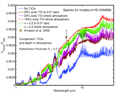
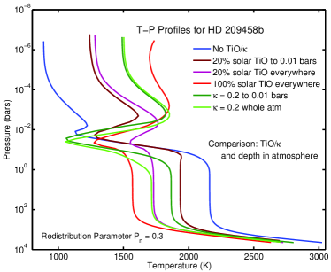
Figure 2: Comparison of the effect of model gaseous TiO in the whole atmosphere versus gaseous TiO only in the upper atmosphere. This figure presents spectra (left panel) and temperature-pressure profiles (right panel) for six models of HD 209458b. Superposed on the spectrum plot are the IRAC data points from Knutson et al. (2008a). There are two models with 20% solar TiO, one of which has this mixing ratio throughout the whole atmosphere and the other with TiO added only above 0.01 bars. There are two models with an absorber, that is gray between $3\times 10^{14}$ and $7\times 10^{14}$ Hz, whose opacity is $\kappa=0.2{\rm~{}cm^{2}~{}g^{-1}}$ (the $\kappa_{e}$ of Burrows et al. 2007a); one has the absorber throughout the whole atmosphere and one has the absorber only above 0.01 bars. Finally, there is both a model with no TiO and a model with solar abundance of TiO throughout the atmosphere. See § 2.1 for a discussion.

We, therefore, neglect the contributions of VO, and investigate what errors in spectra and temperature-pressure profiles are likely to be generated by the model assumption that gaseous TiO exists throughout the atmosphere. Figure 2 portrays spectra (left panel) and temperature-pressure profiles (right panel) for six models of HD 209458b. Superposed on the spectrum plot are the four data points for this planet measured by Knutson et al. (2008a) using the Spitzer InfraRed Array Camera (IRAC). One of the models in this figure is a base case that has no additional upper atmosphere absorber (blue curve); this model does not produce a thermal inversion and fails to match the Knutson et al. (2008a) data. Another model has solar abundance of TiO throughout the atmosphere (red curve); this one has the largest thermal inversion and matches the Knutson et al. (2008a) data the best. The remainder of the models in this figure demonstrate that our assumption that the extra absorber is present throughout the atmosphere does not cause large errors either in predicted emergent spectra or in temperature-pressure profiles. Included on Fig. 2 is a pair of models with 20% solar TiO. One model has this species present from the top of the atmosphere down to 0.01 bars, and the other has it throughout the atmosphere. Finally, there is a pair of models with a gray absorber of opacity $\kappa=0.2\rm~{}cm^{2}~{}g^{-1}$, similar to the $\kappa_{e}$ of Burrows et al. (2008). Again, one model has this absorber from the top of the atmosphere to 0.01 bars and the other has it throughout the atmosphere. The differences in spectra and profiles between the models with absorbers only in the upper atmosphere and those with absorbers throughout the atmosphere are minor enough that for the purposes of this simple study we proceed with models that have the absorber everywhere.

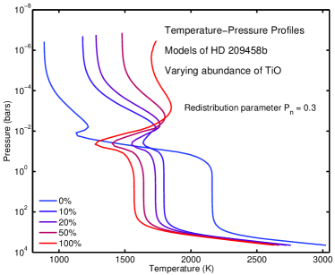
Figure 3: Comparison of different mixing ratios of TiO. This figure shows spectra (left panel) and temperature-pressure profiles (right panel) for five models of HD 209458b: with no TiO, and with 10%, 20%, 50%, and 100% of solar abundance of TiO. Gaseous TiO is assumed throughout the atmosphere, and the redistribution parameter $P_{n}=0.3$ is used for all models. The spectrum plot superposes IRAC data points from Knutson et al. (2008a). As the abundance of TiO increases, the upper atmosphere temperature increases, since it absorbs a greater fraction of incident stellar energy, while the lower atmosphere cools because less of the stellar flux penetrates to depth. The models with 50% and 100% solar abundance TiO have significant thermal inversions in their upper atmospheres; the models with less TiO do not. It is most significant that higher mixing ratios of TiO cause greater planet-star flux ratios over most of the wavelength range. Models with 50% and 100% solar abundance of TiO are decent matches to the IRAC 1 ($\sim$3.6 $\mu$m), IRAC 2 ($\sim$4.5 $\mu$m), and IRAC 3 ($\sim$5.8 $\mu$m) points, though they do fail to match the IRAC 4 ($\sim$8.0 $\mu$m) point. However, the 0%, 10%, and 20% solar TiO models, which lack thermal inversions, entirely fail to match the IRAC data.

Finally, we consider several VO-free models of HD 209458b in order to estimate what mixing ratio of TiO would be required to sustain an upper atmosphere inversion that produces spectra roughly consistent with measured data. Figure 3 presents spectra (left panel) and temperature-pressure profiles (right panel) for five models of HD 209458b, one with no TiO, and others with 10%, 20%, 50%, and 100% solar abundance of TiO. Superposed on the spectrum plot are the four IRAC points from Knutson et al. (2008a). The models with 50% and 100% solar abundance of TiO have thermal inversions in the upper atmosphere and are consistent with the IRAC 1 ($\sim$3.6 $\mu$m), 2 ($\sim$4.5 $\mu$m), and 3 ($\sim$5.8 $\mu$m) points. The fact that none of these models matches all of the observed data shows that our theoretical understanding of radiation from exoplanet atmospheres is incomplete. Nevertheless, one crucial lesson from the data of Knutson et al. (2008b) is that since the IRAC 2 point is significantly higher than the IRAC 1 point, and since the photosphere of IRAC 2 is at greater altitude than that of IRAC 1 (Burrows et al., 2008), the planet would seem ineluctably to have a thermal inversion, other theoretical uncertainties notwithstanding. Fig. 3 suggests that if TiO is the extra absorber its mixing ratio in the upper atmosphere ought to be no less than $\sim$50% of the corresponding solar ratio.

2.2 Modeling Mixing Ratio vs. Altitude

As Fig. 3 shows, any cold-trap regions cannot deplete the atmosphere of Ti too significantly without leaving TiO insufficiently abundant to produce the inferred thermal inversions. How can we estimate how much the cold-trap region depletes the upper atmosphere of TiO? In this section, we describe our model for determining the atmospheric profiles of TiO and the amount of depletion in a turbulent cold-trap region. To do so, we introduce the turbulent diffusion coefficient $K_{zz}$ (Colegrove et al., 1965; Lewis & Fegley, 1984; Noll et al., 1988; Drossart et al., 1990; Rodrigo et al., 1990). $K_{zz}$ parameterizes, in a single number, a variety of processes (including turbulence and other forms of macroscopic mixing) that act for each species to equalize the number density (or partial pressure) at different spatial locations.

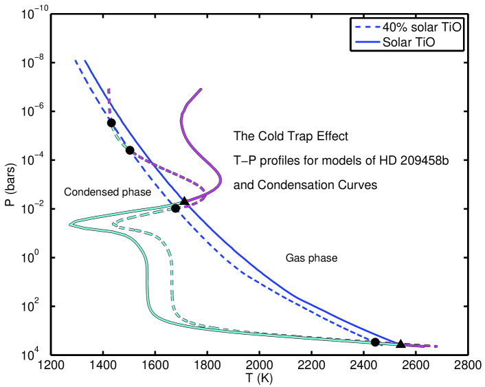
Figure 4: The TiO cold-trap. Condensation curves (blue) and temperature-presure profiles of models of HD 209458b (cyan and magenta) are shown for two mixing ratios of TiO – 40% solar (dashed) and 100% solar (solid). The profiles are calculated assuming TiO is present in the entire atmosphere at the specified mixing ratio. Magenta (cyan) parts of the profiles indicate where the atmosphere is warmer (colder) than the corresponding condensation curve and, therefore, where titanium is in the gaseous TiO (condensed) phase. Filled circles (triangles) mark the intersections of the 40% (100%) solar mixing ratio profile with the corresponding condensation curve. Notice that, at 40% solar titanium, the atmosphere of HD 209458b might have two titanium cold-traps, whereas at 100% solar it has just one.

We start by identifying the cold-trap region(s). On the day side, there are in general three regions: $(i)$ the hot, isentropic convection zone, which contains gaseous TiO; $(ii)$ the cold trap, which contains titanium condensates; and, $(iii)$ the hot, thermally inverted upper atmosphere, in which TiO is gaseous. Depending on a planet’s temperature-pressure profile, it might also have no cold-traps. The phase of titanium compounds as a function of altitude in a planet’s atmosphere is found by comparing the planet’s temperature-pressure profile with the titanium condensation curve for the corresponding metallicity. TiO is gaseous where the atmosphere is hotter than the condensation curve and titanium is in condensed form where the atmosphere is cooler than the condensation curve. These condensation curves vary with metallicity. At a given pressure, higher metallicity causes the condensation curve to be at a higher temperature. Figure 4 illustrates, in the context of HD 209458b, how the comparison of profiles to condensation curves yields the location of cold-trap regions. Models of this planet with 40% solar TiO and with 100% solar TiO are presented, along with the corresponding condensation curves (Sharp & Burrows, 2007). The points of intersection are demarcated, and cold-trap regions are indicated by cyan regions of the profile curves. For example, on HD 209458b in the two profiles shown the largest cold-trap region extends from roughly $3\times 10^{3}$ bars to $10^{-2}$ bars.

In order to understand how much Ti reaches the upper atmosphere of an EGP, we start by considering the vertical distribution of different molecular species in an atmosphere with a variety of chemical constituents. For a particular molecular species $i$ (where $i$ could be TiO, H₂, or any other atmospheric constituent), the vertical abundance profile $n_{i}[z]$ varies with time as $\partial n_{i}/\partial t=-\nabla\cdot\vec{F}_{i}~{}(\rm+~{}sources_{i}~{}-~{}sinks_{i})$, where $n_{i}[z]$ is the number density of species $i$ as a function of altitude $z$, and $\vec{F}_{i}$ is the flux of species $i$. If we ignore sources and sinks, and express the flux as a combination of molecular and turbulent diffusion with gravitational settling, as per Brewer (1949) and Chamberlain & Hunten (1987), then we may write the rate of change of the vertical distribution of species $i$ as follows:

$$\frac{\partial n_{i}[z]}{\partial t} = \frac{\partial}{\partial z}\left\{D_{i}\left(\frac{\partial n_{i}}{\partial z}+\left(\frac{\partial\ln T}{\partial z}+\frac{m_{i}g}{kT}\right)n_{i}\right)\right.$$ (1)

$$\left.+K_{zz}\left(\frac{\partial n_{i}}{\partial z}+\left(\frac{\partial\ln T}{\partial z}+\frac{\mu m_{p}g}{kT}\right)n_{i}\right)\right\}.$$

In this equation, $D_{i}$ is the coefficient of molecular diffusion, $m_{i}$ is the molecular weight, $\mu m_{p}$ is the product of the mean molecular weight ($\mu$) and the mass of a proton ($m_{p}$), $g$ is the gravitational acceleration (assumed to be constant), $k$ is Boltzmann’s constant, $T$ is the temperature, and $K_{zz}$ is the coefficient of turbulent diffusion in the vertical direction.

The timescale for achieving steady state in a diffusion problem with eddy diffusion coefficient $K_{zz}$ is given by the square of a characteristic length divided by $K_{zz}$ (Griffith & Yelle, 1999):

$$\tau_{\rm ss}\sim L^{2}/K_{zz}\,.$$ (2)

A characteristic vertical length scale is the pressure scale height

$$H_{P}\equiv\frac{kT}{\mu m_{p}g}\,,$$ (3)

which is not more than $\sim$10⁸ cm (1000 km) for EGPs. $K_{zz}$ is not well constrained. A variety of estimates of $K_{zz}$ for Jupiter’s atmosphere place it in the range $10^{2}-10^{9}\rm~{}cm^{2}~{}s^{-1}$ (Bézard et al., 2002; Fegley & Lodders, 1994; Ackerman & Marley, 2001; Ben Jaffel et al., 2007). Estimates in the context of brown dwarfs place it in the range $10^{2}-10^{6}\rm~{}cm^{2}~{}s^{-1}$ (Saumon et al., 2006, 2007; Griffith & Yelle, 1999; Hubeny & Burrows, 2007). If highly irradiated EGPs are at least as vigorously mixed as Jupiter and brown dwarfs are thought to be, then we may find an upper bound for $\tau_{\rm ss}$ by setting $K_{zz}\;\hbox to0.0pt{\lower 2.5pt\hbox{$\sim$}\hss}\raise 1.5pt\hbox{$>$}\;10^{2}\rm~{}cm^{2}~{}s^{-1}$ in eq. (2):

$$\tau_{\rm ss}\;\hbox to0.0pt{\lower 2.5pt\hbox{$\sim$}\hss}\raise 1.5pt\hbox{$<$}\;10^{14}~{}\rm s\sim 3~{}\rm Myr\ll\tau_{\rm planet~{}age}\,,$$ (4)

where $\tau_{\rm planet~{}age}$ is the planet’s age. This indicates that, in much less than a planet’s age (hundreds of megayears to a gigayear or more), the atmosphere has reached a steady state and $\partial n_{i}/\partial t=0$. We further assume that the mean net fluxes are zero in the steady state. Equation (1) may, therefore, be rewritten as follows:

$$D_{i}\left(\frac{\partial P_{i}}{\partial z}+\frac{m_{i}g}{kT}P_{i}\right)+K_{zz}\left(\frac{\partial P_{i}}{\partial z}+\frac{\mu m_{p}g}{kT}P_{i}\right)=0\,.$$ (5)

Here, the $n_{i}$ of eq. (1) has been replaced by the partial pressure of species $i$, $P_{i}$, in accordance with the ideal gas law.

The general solution to this equation is

$$P_{i}[z]=P_{i}[z_{0}]\exp\left[-\int_{z_{0}}^{z}d\zeta\frac{(m_{i}/\mu m_{p})D_{i}+K_{zz}}{H_{P}[\zeta](D_{i}+K_{zz})}\right],$$ (6)

where $z_{0}$ is an arbitrary reference height. In general, $T$, $\mu$, $D_{i}$, and $K_{zz}$ are functions of $z$. Notice that eq. (6) indicates that if vertical mixing is vigorous ($K_{zz}\gg D_{i}$), all species will have the same vertical scale height $H_{P}$. Conversely, in the absence of macroscopic mixing ($K_{zz}\ll D_{i}$), gravitational settling of heavier molecules will cause each species to have its own pressure scale height $H_{P_{i}}\approx H_{P}/(m_{i}/\mu m_{p})$.

Since the total pressure varies as

$$p[z]=p[z_{0}]\exp\left[-\int_{z_{0}}^{z}d\zeta/H_{P}[\zeta]\right],$$ (7)

the mixing ratio of species $i$, $Y_{i}\equiv P_{i}/P$, may be expressed as

$$Y_{i}[z] = Y_{i}[z_{0}]\exp\left[-\int_{z_{0}}^{z}d\zeta\left\{\frac{(m_{i}/\mu m_{p})D_{i}+K_{zz}}{H_{P}[\zeta](D_{i}+K_{zz})}-\frac{1}{H_{P}[\zeta]}\right\}\right]$$ (8)

$$= Y_{i}[z_{0}]\exp\left[-\int_{z_{0}}^{z}\frac{d\zeta}{H_{P}[\zeta]}\frac{\left\{(m_{i}/\mu m_{p})-1\right\}D_{i}}{D_{i}+K_{zz}}\right].$$

Equation (8) has the same general form as eq. (6), which prompts us to define a “scale height of the mixing ratio” $H_{Y_{i}}$ as follows:

$$H_{Y_{i}}[z]\equiv H_{P}[z]\frac{D_{i}+K_{zz}}{D_{i}\left\{(m_{i}/\mu m_{p})-1\right\}}\,.$$ (9)

We consider the behavior of this model in cases where $K_{zz}$ is large and where it is small relative to $D_{i}$. If $K_{zz}\gg D_{i}$, then $H_{Y_{i}}\gg H_{P}$, which indicates that the mixing ratio of species $i$ remains essentially constant with height, as is expected with vigorous mixing. If $K_{zz}\ll D_{i}$, the scale height of the mixing ratio $H_{Y_{i}}\approx H_{P}/\left\{(m_{i}/\mu m_{p})-1\right\}$, which indicates that the $e$-folding height for the mixing ratio of each species is roughly inversely proportional to its molecular weight, which we take to be 2.3 in all models.

Presumably, the deep interior of an EGP is well-mixed by convection, with $Y_{i}$ constant with $z$ for all species $i$. In the atmosphere, a useful metric of the abundance of a species is its mixing ratio relative to its mixing ratio at depth:

$$f[z]\equiv\frac{Y_{i}[z]}{Y_{i}[0]},$$ (10)

where $z=0$ is taken to be the radiative-convective boundary.

2.2.1 Vertical Distribution of Gaseous Species

In regions where TiO is gaseous, how does its mixing ratio vary with altitude? In accordance with Kittel (1969) we estimate the diffusivity of TiO through molecular hydrogen as

$$D_{\rm TiO}\sim\frac{\lambda\langle v\rangle}{3}\,,$$ (11)

where $\lambda$ is the mean free path and $\langle v\rangle$ is the mean velocity. We estimate the mean free path as $\lambda\sim 1/(n\sigma)$, where $\sigma$ is the cross-section for collision. Taking as a typical cross-section $\sigma\sim\pi(1\rm~{}\AA)^{2}$, and as a typical speed $\langle v\rangle\sim(8kT/3m_{\rm TiO})^{1/2}$, we estimate $D_{\rm TiO}\sim 90\rm~{}cm^{2}~{}s^{-1}$ at 1500 K and 1 bar. Similarly, this argument suggests that at kilobar pressures $D_{\rm TiO}$ is in the range of $\sim$10${}^{-1}\rm~{}cm^{2}~{}s^{-1}$, whereas at millibar pressures, it is in the range of $\sim$10${}^{5}\rm~{}cm^{2}~{}s^{-1}$. This simple estimate predicts comparable molecular diffusion values to those calculated in Rodrigo et al. (1990) in the context of the Earth’s thermosphere.

We now consider several possible cases of relative magnitudes of molecular and turbulent diffusion:

1. If there is no turbulent mixing, or if $K_{zz}\ll D_{\rm TiO}$, eq. (9) implies that $H_{Y_{\rm TiO}}\approx H_{P}/27$. On HD 209458b, $H_{P}\sim 500-600\rm~{}km$. As a result, if $K_{zz}\ll D_{\rm TiO}$, the scale height of the mixing ratio $H_{Y_{\rm TiO}}\sim 20$ km. In the $\sim$14 pressure scale heights from a kilobar to a millibar, the mixing ratio would drop by $\sim$370 $e$-foldings. In short, without macroscopic mixing, $f_{\rm TiO}=0$ at the top of the atmosphere.

2. At the opposite extreme, if $K_{zz}\ggg D_{\rm TiO}$, the mixing ratio of even a heavy molecule remains essentially constant so long as the species is in the gas phase. If, for example, $K_{zz}=10^{4}(D_{\rm TiO})$, eq. (9) implies that $H_{Y_{\rm TiO}}\approx 370H_{P}$. In this case, in a vertical distance of $\sim$14 pressure scale heights the mixing ratio of TiO would decrease by only $\sim$4%.

3. Finally, consider a regime wherein $K_{zz}$ is somewhat, but not overwhelmingly, larger than $D_{\rm TiO}$. If this is the case, $f_{\rm TiO}$ might be neither $\sim$0 nor $\sim$1, but rather an interesting intermediate value. Indeed, since the mean free path varies inversely with number density – and, therefore, $D$ varies roughly with $\sim p^{-1}$ – it seems likely that there are some regions of an EGP’s atmosphere that are in this regime. For example, if $K_{zz}=10D_{\rm TiO}$ at some altitude, then $H_{Y_{\rm TiO}}\sim 0.41H_{P}$. This would imply that the mixing ratio drops off with altitude more precipitously than pressure does, but not dramatically more. If, at another altitude, $K_{zz}=100D_{\rm TiO}$, then $H_{Y_{\rm TiO}}\sim 3.7H_{P}$. This would imply that the mixing ratio decreases with altitude more gradually than pressure does.

In the general case, where TiO is in the gas phase $f_{\rm TiO}$ varies with altitude according to the following equation:

$$\ln[f_{i}]=-\int_{z_{0}}^{z}\frac{d\zeta}{H_{P}[\zeta]}\frac{\left\{(m_{i}/\mu m_{p})-1\right\}D_{i}}{D_{i}+K_{zz}}\,.$$ (12)

2.2.2 Vertical Distribution of Condensed Species

In the cold-trap region, titanium is in condensate form. Details of the chemistry by which TiO condenses into a variety of Ti-bearing compounds can be found in Lodders (2002). Because of the complicated nature of the condensation chemistry, it is difficult to specify exactly which condensates form and in what quantity. Therefore, we will simply use the subscript $c_{i}$ to denote the condensates of species $i$. We assume that the condensates will form roughly spherical condensates of radius $a$. Lacking a first-principles theory for the process of condensate formation, we cannot predict the size-distribution or the modal value of particle radii. Instead, we use a wide range of values of $a$ that spans several orders of magnitude: $0.1~{}\mu{\rm m}\leq a\leq 100~{}\mu{\rm m}$. To model the distribution of these condensates, we start with an expression analogous to eq. (1), only for the condensed form of species $i$, taking $n_{c_{i}}$ to be the number density of condensates of species $i$. If we consider the cloud of condensates to be a gas, it is an extremely rarified one. To a good approximation, it should, therefore, behave as an ideal gas. The “partial pressure” of condensates of species $i$ is then approximately given by the ideal gas law: $P_{c_{i}}\approx n_{c_{i}}kT$.

The argument that the atmosphere has achieved steady state applies here as well. Therefore, we proceed in the same manner as before, by setting the vertical flux of condensates equal to zero and solving for $P_{c_{i}}$. The solution is given by an expression identical to eq. (6), except with $m_{i}$ and $D_{i}$ replaced by $m_{c_{i}}$ and $D_{c_{i}}$.

The background pressure is again given by eq. (7). If $N_{c_{i}}\equiv m_{c_{i}}/m_{i}$ is the number of atoms/molecules of species $i$ per condensates, then, following eq. (8), the mixing ratio in a cold-trap region may be written

$$Y_{c_{i}} \equiv N_{c_{i}}\frac{P_{c_{i}}}{P}$$ (13)

$$= Y_{i}[0]\exp\left[-\int_{0}^{z}\frac{d\zeta}{H_{P}[\zeta]}\frac{\left\{(m_{c_{i}}/\mu m_{p})-1\right\}D_{c_{i}}}{D_{c_{i}}+K_{zz}}\right].$$

The ratio of the mixing ratio $f_{i}$ of species $i$ to its value at depth may be written,

$$f[z]=\frac{Y_{c_{i}}}{Y[0]}\,.$$ (14)

Equation (13) may be simplified by making use of the low Reynolds number expression for terminal velocity, appropriate for an EGP’s atmosphere (Ackerman & Marley, 2001; Showman et al., 2008b). In this regime, the viscous drag force, balanced by gravity, is $F_{v}=6\pi\eta av$, where $\eta$ is the dynamic viscosity, $a$ the particle size, and $v$ the speed of the particle through the viscous medium. This expression implies a terminal velocity of

$${v_{f}}_{\rm Stokes}=\frac{2}{9}\frac{a^{2}\rho_{c_{i}}g}{\eta}.$$ (15)

We estimate the molecular diffusivity of condensates $D_{c_{i}}$ using the Stokes-Einstein relation:

$$D_{\rm Stokes}=\frac{kT}{6\pi\eta a}\,.$$ (16)

Equation (16) is valid in the low-Reynolds number regime only when the mean free path of the molecules constituting the fluid is small compared to the size of the falling body. When this ratio, called the Knudsen number ($N_{\rm Kn}\equiv\lambda/a$; Knudsen & Weber 1911) is not small, a correction is needed. The analysis of small particles moving through highly rarified media has a long history, dating back to early theoretical work by Cunningham (1910) and contemporaneous experimental work (Millikan., 1913; Millikan, 1923). The form of the Cunningham-Millikan-Davies “slip factor correction” (Davies, 1945) has been updated somewhat over the years (El-Fandy, 1953; Baines et al., 1965). We adopt the value from Li & Wang (2003):

$$\beta=1+N_{\rm Kn}(1.256+0.4\exp[-1.1/N_{\rm Kn}])\,.$$ (17)

In the nonzero Knudsen number regime, the true terminal velocity and diffusivity are increased over the Stokes values (eqs. 15 and 16) by a factor of $\beta$:

$$v_{f} = \beta{v_{f}}_{\rm Stokes}$$ (18)

$$D = \beta D_{\rm Stokes}\,.$$ (19)

Substituting eq. (18) into eq. (19), and noting that $m_{c_{i}}=(4/3)\pi(a_{c_{i}})^{3}\rho_{c_{i}}$, we have

$$(m_{c_{i}}/\mu m_{p})D_{c_{i}} = v_{f}kT/(\mu m_{p}g)$$ (20)

$$= \beta{v_{f}}_{\rm Stokes}H_{P}.$$

When eq. (20) is substituted into the expression for $H_{Y_{c_{i}}}$, the result is

$$H_{Y_{c_{i}}}^{*}[z]=H_{P}[z]\frac{D_{c_{i}}+K_{zz}}{\beta{v_{f}}_{\rm Stokes}H_{P}(1-\mu m_{p}/m_{c_{i}})}=\frac{D_{c_{i}}+K_{zz}}{\beta{v_{f}}_{\rm Stokes}(1-\mu m_{p}/m_{c_{i}})}\,.$$ (21)

Equation (19) implies that $D_{c_{i}}=4.4\times 10^{-7}{\rm~{}cm^{2}~{}s^{-1}}\beta(a/1{\mu\rm m})^{-1}(T/1500~{}\rm K)(\eta/2.5\times 10^{-4}{\rm~{}g~{}cm^{-1}})$. If $K_{zz}\gg D_{c_{i}}$ and $m_{c_{i}}\gg\mu m_{p}$, then

$$H_{Y_{c_{i}}}^{*}[z]\approx\frac{K_{zz}}{\beta{v_{f}}_{\rm Stokes}}\,.$$ (22)

This implies that, at the top of a cold-trap of vertical extent $z-z_{0}$,

$$\ln[f_{i}]=-\int_{z_{0}}^{z}\frac{d\zeta}{K_{zz}/(\beta{v_{f}}_{\rm Stokes})}\,.$$ (23)

3 Results

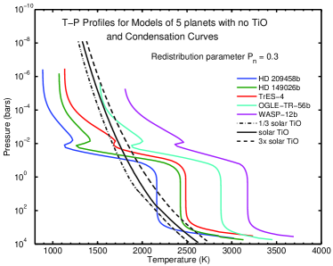
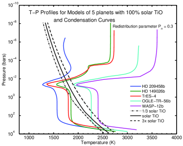
Figure 5: Comparison of temperature-pressure profiles for models of five planets with no TiO (left panel) and with solar abundance of TiO (right panel). This figure shows $T$-$P$ profiles for models without (left panel) and with (right panel) the strong optical absorber TiO, for HD209458b (blue), HD149026b(green), TrES-4 (red), OGLE-TR-56b (cyan), and WASP-12b (magenta). The redistribution parameter $P_{n}$ is set equal to = 0.3. Condensation curves (black) for titanium are superposed, showing the locations of the condensation curves at 0.32 solar abundance (dashed-dotted line), solar abundance (solid line), and 3.2 times solar abundance (dashed line). The addition of TiO heats the upper atmosphere and cools the lower atmosphere, because more of the incident stellar flux is absorbed high in the atmosphere.

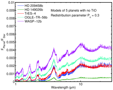
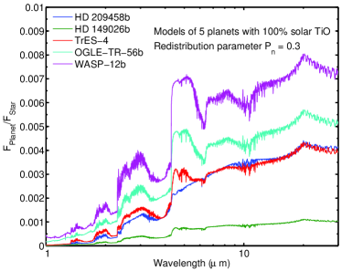
Figure 6: Comparison of spectra for models of five planets with no TiO (left panel) and with solar abundance of TiO (right panel). This figure presents the spectra that correspond to the $T$-$P$ profiles in Fig. 5, for the same five planets. Here, adding TiO increases the planet-star flux ratios in most of the IRAC range. In particular, the flux ratios for IRAC 2 ($\sim$4.5 $\mu$m) and IRAC 3 ($\sim$5.8 $\mu$m) are significantly increased.

Titanium oxide, if present in a highly irradiated EGP’s atmosphere, can have a dramatic influence on both the temperature-pressure profile and the emergent spectrum. Figures 2 and 3 show this in the context of HD 209458b. However, there are other exoplanets where stellar irradiation, and, hence, the influence of gaseous TiO, could be even stronger. This can be seen in the sharp contrasts displayed between the two panels of both Figs. 5 and 6.

Figures 5 and 6 both show models of five planets: 1) HD 209458b (Henry et al., 2000), which receives incident flux of $\sim 10^{9}\rm~{}erg~{}cm^{-2}~{}s^{-1}$; 2) HD 149026b (Sato et al., 2005), which receives $\sim$2$\times 10^{9}\rm~{}erg~{}cm^{-2}~{}s^{-1}$; 3) TrES-4 (Mandushev et al., 2007), which receives $\sim$2$\times 10^{9}\rm~{}erg~{}cm^{-2}~{}s^{-1}$; 4) OGLE-TR-56b (Udalski et al., 2002), which receives $\sim$6$\times 10^{9}\rm~{}erg~{}cm^{-2}~{}s^{-1}$; and 5) WASP-12b (Hebb et al., 2008), which receives $\sim$9$\times 10^{9}\rm~{}erg~{}cm^{-2}~{}s^{-1}$ . The mean molecular weight $\mu$ is taken to be 2.3 for all planets, and $\log_{10}g$ is taken to be 3.00, 3.19, 2.86, 3.27, and 3.04, for HD 209458b, HD 149026b, TrES-4, OGLE-TR-56b, and WASP-12b, respectively (where $g$ is in $\rm cm~{}s^{-2}$). (See Table 1 for a summary of these values.)

Figure 5 presents temperature-pressure profiles for models of these planets with no TiO (left panel) and with solar abundance of TiO (right panel). Figure 6 portrays spectra for the corresponding models. We note that, as described in §2.1, models with TiO contain solar abundance of TiO throughout the atmosphere, including in the cold trap; this procedure should not produce large errors. In the profile plots (Fig. 5) contain condensation curves for titanium at 0.32 solar abundance (dashed-dotted black curve), solar abundance (solid black curve), and 3.2 times solar abundance (dashed black curve). In the left panel, there is no cold-trap, because there is no TiO. In the right panel, as in Fig. 4, cold-trap regions are found where each planet’s profile is on the cold side of the solar abundance condensation curve. The solar abundance TiO models for HD 209458b, HD 149026b, TrES-4, and OGLE-TR-56b all have cold-trap regions. Since the model for WASP-12b with solar abundance TiO is never colder than the corresponding condensation curve, our model predicts that WASP-12b would not have a day-side cold trap for titanium if it is at or near solar abundance. Figure 6 shows that in all five model planets, solar abundance TiO produces a large thermal inversion in the upper atmosphere (and cools the lower atmosphere). This is reflected in the spectrum as an increase in planet-star flux ratio throughout much of the near infrared.

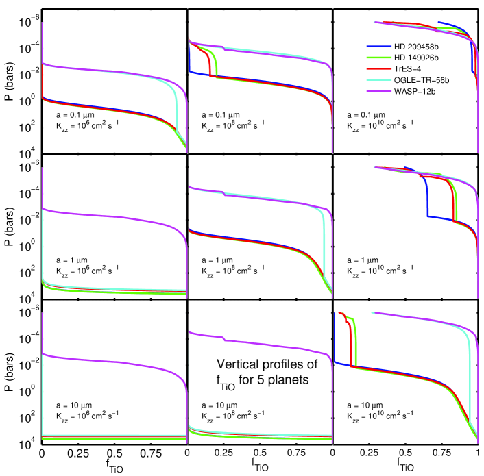
Figure 7: Vertical profiles of $f_{\rm TiO}$ for five planets. $f_{\rm TiO}$ (abscissa) is shown as a function of pressure (ordinate) for different combinations of particle size $a$ and turbulent diffusion coefficient $K_{zz}$. Left-to-right, $K_{zz}$ takes on the values $10^{6}\rm~{}cm^{2}~{}s^{-1}$, $10^{8}\rm~{}cm^{2}~{}s^{-1}$, and $10^{10}\rm~{}cm^{2}~{}s^{-1}$. Top-to-bottom, $a$ varies from 0.1 $\mu$m to 1 $\mu$m to 10 $\mu$m. HD 209458b, HD 149026b, TrES-4, OGLE-TR-56b, and WASP-12b are represented, respectively, with dark blue, green, red, cyan, and magenta (same color scheme as in Figs. 5 and 6). Since WASP-12b has no day-side cold trap in our models, its curves are independent of $a$. At $K_{zz}=10^{6}\rm~{}cm^{2}~{}s^{-1}$, none of the model planets has any appreciable amount of TiO in the upper atmosphere.

How much TiO is likely to survive the cold-traps on these planets and to reach the upper atmospheres? In Figs. 7 through 10, we address this question.

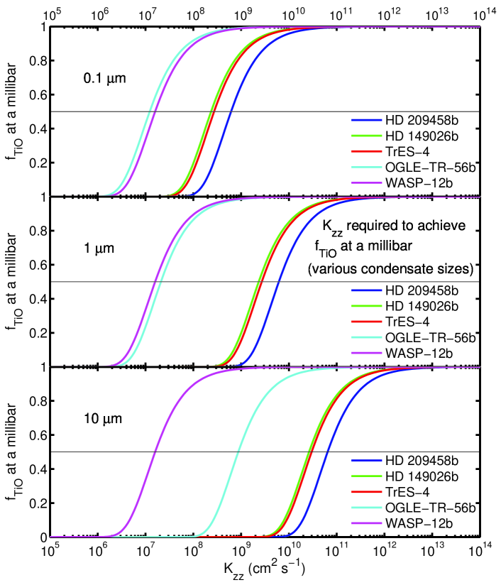
Figure 8: $K_{zz}$ required to achieve $f_{\rm TiO}$ at $p=10^{-3}$ bars, for five planets, for various condensate particle sizes. For condensates ranging from 0.1 $\mu$m (top panel) to 10 $\mu$m (bottom panel), $f_{\rm TiO}$ is plotted as a function of $K_{zz}$ on each of the five planets considered in this paper (same color scheme as in previous figures). The magenta curve for WASP-12b is independent of particle size and so is identical in all three panels. A horizontal black line is shown in each plot at $f_{\rm TiO}=0.5$ to aid the eye in identifying the value of $K_{zz}$ that is required to achieve this fiducial relative mixing ratio.

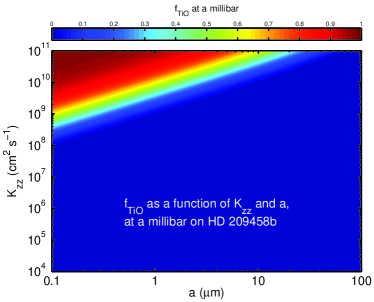
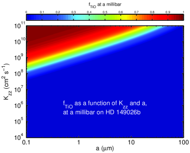
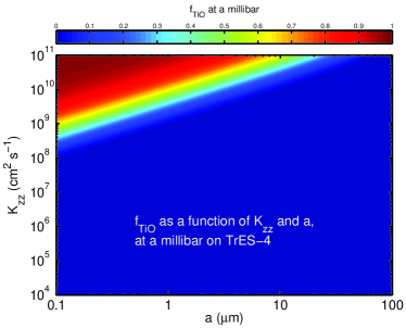
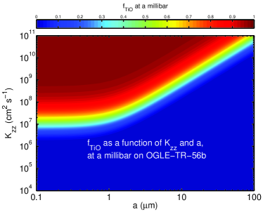
Figure 9: Color-map of $f_{\rm TiO}$ at a millibar, as a function of $a$ and $K_{zz}$ on the four planets with day-side cold traps (HD 209458b: top-left; HD 149026b: top-right; TrES-4: bottom-left; OGLE-TR-56b: bottom-right). The color contours indicate the mixing ratio of TiO at $10^{-3}$ bars relative to the interior mixing ratio of titanium, for various combinations of particle size (0.1-100 $\mu$m) and turbulent diffusion coefficient ($10^{4}$-$10^{11}\rm~{}cm^{2}~{}s^{-1}$). The green band indicates the combinations required to achieve the fiducial value of $f_{\rm TiO}\sim 0.5$.

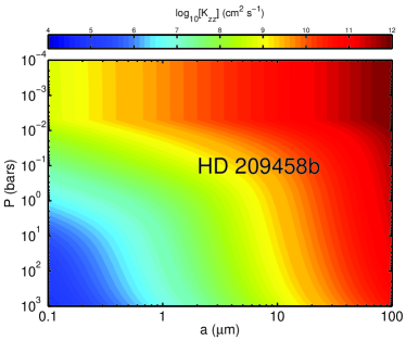
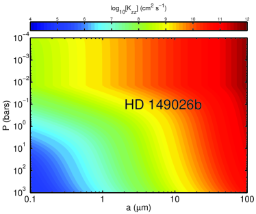
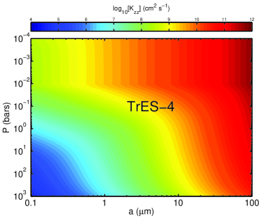
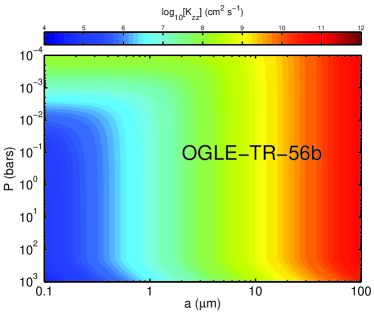
Figure 10: Color-map of $\log[K_{zz}]$ (in $\rm cm^{2}~{}s^{-1}$) required to achieve $f_{\rm TiO}=0.5$, as a function of $a$ and $P$ on the four planets with day-side cold traps (HD 209458b: top-left; HD 149026b: top-right; TrES-4: bottom-left; OGLE-TR-56b: bottom-right).

Figures 7-10 all show the results of integrating eq. (23) for different assumed values of $a$ and $K_{zz}$ (and for the different $T$-$P$ profiles of the different planet models). The $T$-$P$ profile (which is determined by finding a radiative equilibrium solution to the radiative transfer equation in a plane-parallel atmosphere, as described in §2.1 and in the cited references) is related to altitude through the scale height relationship of eq. (3). Terminal velocities $v_{f}$ are calculated with eqs. (15) and (17).

Figure 7 illustrates how much turbulent mixing is required to achieve nonzero concentrations of TiO at the top of the atmosphere of each of the five planets under consideration in this paper. This figure presents vertical profiles of $f_{\rm TiO}$ for various combinations of $a$ (top-to-bottom: 0.1 $\mu$m to 1 $\mu$m to 10 $\mu$m) and $K_{zz}$ (left-to-right: $10^{6}\rm~{}cm^{2}~{}s^{-1}$ to $10^{8}\rm~{}cm^{2}~{}s^{-1}$ to $10^{10}\rm~{}cm^{2}~{}s^{-1}$). Since WASP-12b has no day-side cold trap in our models, its curves are independent of $a$. To achieve nonzero concentrations of TiO at microbar pressures requires values of $K_{zz}$ that are very high for a stably stratified region such as the radiative part of an EGP’s atmosphere ($K_{zz}\;\hbox to0.0pt{\lower 2.5pt\hbox{$\sim$}\hss}\raise 1.5pt\hbox{$>$}\;10^{10}\rm~{}cm^{2}~{}s^{-1}$, even for WASP-12b, with no day-side cold trap). To achieve a nonzero concentration of TiO at millibar pressures, the requirements on $K_{zz}$ are not quite so extreme, but even still $K_{zz}$ must be  $\sim$$>$ 10${}^{8}\rm~{}cm^{2}~{}s^{-1}$, even for the smallest particle sizes, on all but the hottest planets (OGLE-TR-56b and WASP-12b). At $K_{zz}=10^{6}\rm~{}cm^{2}~{}s^{-1}$, none of the planets has any appreciable amount of TiO in the upper atmosphere, and only OGLE-TR-56b and WASP-12b have nonzero TiO above $\sim$1 bar, even for $a=0.1~{}\mu$m.

As can be seen in Figs. 1-3 and Fig. 5, the thermal inversions reach maximum temperatures at roughly millibar pressures. This indicates that $f_{\rm TiO}$ ought to be nonzero at these pressures. But what nonzero value is required? Because, as Figs. 8 and 9 demonstrate, $f_{\rm TiO}$ transitions from $\sim$0 to $\sim$1 in a fairly narrow range of $K_{zz}$, a reasonable estimate is that, to cause a thermal inversion, $f_{\rm TiO}$ should be $\sim$0.5 at $p\sim 10^{-3}$ bars.

Another way to visualize the analysis of Fig. 7 is to ask how $f_{\rm TiO}$ varies with $K_{zz}$ at a particular pressure level. Figure 8 portrays this relationship at a millibar, on the same five planets, for condensate particle sizes 0.1 $\mu$m (top), 1 $\mu$m (middle), and 10 $\mu$m (bottom). The amount of turbulent mixing required to achieve a given $f_{\rm TiO}$ tends to increase with particle size. The magenta curve for WASP-12b, however, is independent of particle size and is, therefore, the same in all three panels. This figure shows that $f_{\rm TiO}$ is nearly 0 or nearly 1 for most values of $K_{zz}$, and makes the transition over roughly an order of magnitude change in $K_{zz}$. For condensates of radius 10 $\mu$m, even OGLE-TR-56b requires $K_{zz}\sim 10^{9}\rm~{}cm^{2}~{}s^{-1}$, while the other three planets with day-side cold traps (HD 209458b, HD 149026b, and TrES-4) require $K_{zz}$ between $10^{10}$ and $10^{11}\rm~{}cm^{2}~{}s^{-1}$.

Figure 9 displays how the millibar-level value of $f_{\rm TiO}$ varies with $a$ and $K_{zz}$, for the four planets with day-side cold traps. The color contours indicate the mixing ratio of TiO at $10^{-3}$ bars relative to the interior mixing ratio of titanium. The green band indicates the combinations required to achieve the fiducial value of $f_{\rm TiO}\sim 0.5$. This figure shows that planets transition from $f_{\rm TiO}\sim 0$ to $f_{\rm TiO}\sim 1$ in a fairly narrow range of values of $a$ and $K_{zz}$. In general, smaller particles and more vigorous mixing produce larger values of $f_{\rm TiO}$ at a millibar.

One more way to frame this result is to ask what value of $K_{zz}$ is required to bring 50% of the interior mixing ratio of TiO up to a given pressure. Figure 10 shows precisely this. For the four planets with day-side cold traps, color contours indicate the amount of turbulent mixing needed to achieve $f_{\rm TiO}=0.5$, as a function of $a$ and $P$. At millibar pressures, each of these planets requires from $\sim$10${}^{7}\rm~{}cm^{2}~{}s^{-1}$ of turbulent mixing (in the case 0.1-$\mu$m particles in the cold trap of OGLE-TR-56b) to $\sim$10${}^{12}\rm~{}cm^{2}~{}s^{-1}$ (in the case of 100-$\mu$m particles in the cold trap of HD 209458b).

Table 1 also presents the value of the eddy diffusion coefficient $K_{zz}$ that is required to maintain $f_{\rm TiO}=0.5$ above the day-side cold-trap, for various assumed condensate sizes. 0.1-$\mu$m particles require from $K_{zz}\sim 10^{7}\rm~{}cm^{2}~{}s^{-1}$ (in the case of OGLE-TR-56b) to $\sim$10${}^{9}\rm~{}cm^{2}~{}s^{-1}$ (in the case of HD 209458b), and these values increase roughly linearly with particle radius. 1-$\mu$m particles require $K_{zz}\sim 10^{7}$ to $\sim$10${}^{10}\rm~{}cm^{2}~{}s^{-1}$; and 10-$\mu$m particles require $K_{zz}\sim 10^{9}$ to $\sim$10${}^{11}\rm~{}cm^{2}~{}s^{-1}$.

Since we lack constraints on both $a$ and $K_{zz}$, our uncertainty spans many orders of magnitude. Particle radii from 0.1 $\mu$m to 30 $\mu$m or more are not implausible, nor are values of $K_{zz}$ from 10² to 10${}^{9}\rm~{}cm^{2}~{}s^{-1}$, possibly even greater. Only for a narrow range of $a$-$K_{zz}$ space is the upper atmosphere abundance of TiO at all sensitive to $a$ and $K_{zz}$. For most of parameter space, there is either not nearly enough upper atmosphere TiO to cause thermal inversions, or easily enough.

4 Caveats

What should we conclude from the results in §3? In this section, we address a few additional complications of our analysis. First, in §4.1, we consider how a more sophisticated analysis would treat the single-zone model, which considers motions only in the vertical direction, presented in §2. Then, in §4.2, we qualitatively describe how horizontal winds, which effectively couple the day side of a planet to colder parts (including both the night side and the polar regions), influence the day-side upper atmosphere abundance of TiO.

4.1 Caveats for the Single-Zone Model

First, the models presented in §3 assume either solar abundance of TiO or no TiO, but a planet’s interior mixing ratio of titanium might be super-solar. If so, then $f_{\rm TiO}$ could be lower than 0.5 while still maintaining a 50% solar mixing ratio of titanium in the upper atmosphere. If a planet’s interior titanium abundance were twice solar, for instance, $f_{\rm TiO}$ could be 0.25 for a 50% solar mixing ratio of titanium at the top of the cold trap. Nonetheless, the band in $a$-$K_{zz}$ space in which $f$ changes by a factor of two from, say, 0.5 to 0.25, is fairly narrow in comparison to the range of plausible values. Even an order of magnitude change from 0.5 to 0.05 corresponds to a fairly modest change in $K_{zz}$ of a factor of $\sim$3.

It is also conceivable that we dismiss too quickly the possibility that VO contributes significantly to thermal inversions. According to Sharp & Burrows (2007), vanadium condenses at somewhat lower temperature than titanium. All else being equal, its cold-trap would, therefore, be smaller. Still, since even 10 times solar abundance of VO does not produce as large a thermal inversion as has been inferred from observations of HD 209458b it is unlikely that VO could play a key role in producing thermal inversions.

There are two ways in which our analysis is not self-consistent, both related to the false assumption in most of Figs. 1-5 that TiO is present at constant mixing ratio throughout a planet’s entire atmosphere. First, we use the temperature-pressure profiles that result from this assumption to find where the cold-traps are. Second, we also use condensation curves calculated based on this assumption in finding the cold-traps. In reality, as (the non-self-consistently generated) Fig. 7 demonstrates, the mixing ratio of TiO decreases with altitude. Lower abundance of titanium condenses at lower temperature for a given pressure. As a result, the condensation curves of a self-consistent analysis would have shallower slopes that reflect the decrease in mixing ratio of TiO at lower pressures. A more sophisticated model would self-consistently take into account the progressive depletion of TiO in calculating both $T$-$P$ profiles and condensation curves.

Finally, one might ask whether our use of day-side average models could mask the presence of local conditions near the substellar point that are hot enough not to have cold traps. For the four planets that our model predicts have cold traps (HD 209458b, HD 149026b, TrES-4, and OGLE-TR-56b), could the intense insolation near the substellar points raise the temperature enough that the cold traps don’t exist at these local hot spots? As described in Burrows et al. (2008) Appendix D, the average conditions correspond to the ring around the substellar point with direction cosine $\mu=2/3$. However, local conditions at the substellar point (where irradiation is 50% greater than the average used) are such that on HD 209458b, HD 149026b, and TrES-4, the substellar point flux still receives less flux than the day-side average flux received by OGLE-TR-56b, a planet that according to our model has a cold-trap. This suggests that even local 2D models of these 3 planets would have no part of the day side hot enough to avoid having a cold trap. Moreover, parts of the atmosphere with $\mu<2/3$ would have even larger cold traps than predicted by our models. Even if some planets, such as perhaps OGLE-TR-56b, do not have $T$-$P$ profiles corresponding to cold trap conditions at their substellar points, planetary winds would prevent gaseous TiO from remaining at such hot locations for long. Coupling between parts of a planet with different local conditions is the subject of §4.2.

4.2 Other Depletion Regions

The actual process by which planetary atmospheres achieve their spatially and temporally dependent chemical distributions is more complicated than the model presented above. In addition to molecular and turbulent diffusion, planetary-scale winds advect gas and condensates from the day side to the night side and back, equator to pole and back, and across different altitudes. The chemical composition of advected Lagrangian parcels of air can change in response to the local temperature and pressure conditions that they experience in the course of their circulation. The TiO content above the day-side cold-trap, therefore, depends on a variety of timescales: the timescale for zonal circulation, $\tau_{\rm circ}\sim\pi R_{p}/u$, where $u$ is the zonal wind speed; the timescale for gravitational settling of condensates, $\tau_{\rm settle}\sim\Delta z/\beta{v_{f}}_{\rm Stokes}$; the timescale for chemical transitions – the formation and destruction of condensates, $\tau_{\rm chem}$; and the timescale for heating and radiatively cooling, $\tau_{\rm rad}$.

Consider the influence of the night-side cold-trap. The basic formalism for the vertical distribution of a species on the night side (in the absence of advection) is the same as that on the day side. Because the night side has its own temperature-pressure profile (that is on the condensed side of the condensation curve of Ti for most of the atmosphere), it will have its own (advection-free) vertical distribution of species $i$, here labeled $n_{i,\rm n}$. Coupling between the day and night sides may be described quantitatively by adding a source/sink term to eq. (1). This term ought to be proportional to the difference between the number density on the night and day sides, and inversely proportional to the circulation time. In the context of a simple model, suppose that each $z$-level on the day side is carried by circulatory winds to one unique level on the night side (and vice versa). Let $Z_{\rm n}(z)$ be the monotonic, invertible function that maps day-side altitude $z$ to the night-side altitude to which it is coupled. The revised version of eq. (1), then, is the following:

$$\frac{\partial n_{i}[z]}{\partial t} = \frac{\partial}{\partial z}\left\{D_{i}\left(\frac{\partial n_{i}}{\partial z}+\left(\frac{\partial\ln T}{\partial z}+\frac{m_{i}g}{kT}\right)n_{i}\right)\right.$$ (24)

$$\left.+K_{zz}\left(\frac{\partial n_{i}}{\partial z}+\left(\frac{\partial\ln T}{\partial z}+\frac{\mu m_{p}g}{kT}\right)n_{i}\right)\right\}+\frac{n_{i,\rm n}\left[Z_{\rm n}(z)\right]-n_{i}[z]}{\tau_{\rm circ}}.$$

The corresponding equation for the night side looks nearly identical, except 1) a night-to-day coupling function, which is the inverse function of the day-to-night function ($Z_{\rm d}\equiv{Z_{\rm n}}^{-1}$), takes the place of $Z_{\rm n}$; and 2) the sign of the $1/\tau_{\rm circ}$ term is reversed.

For the reasons discussed in §2.2, we still may assume $\partial n_{i}/\partial t=0$. Now, a vertical integration yields

$$D_{i}\left(\frac{\partial n_{i}}{\partial z}+\left(\frac{\partial\ln T}{\partial z}+\frac{m_{i}g}{kT}\right)n_{i}\right)+K_{zz}\left(\frac{\partial n_{i}}{\partial z}+\left(\frac{\partial\ln T}{\partial z}+\frac{\mu m_{p}g}{kT}\right)n_{i}\right)$$

$$+\frac{1}{\tau_{\rm circ}}\int_{0}^{z}\left(n_{i,\rm n}[Z_{\rm n}(\zeta)]-n_{i}[\zeta]\right)d\zeta = 0\,.$$ (25)

We briefly consider the qualitative properties of this equation. An important unknown is the nature of the coupling function $Z_{\rm n}$. This function depends on the trajectories followed by Lagrangian fluid elements that start at different altitudes in the course of their circulation around a planet. Although neither entropy nor pressure is likely to be strictly conserved, are flow patterns best described as isentropic or isobaric?

Since a highly irradiated EGP’s night side lacks the day side’s intense external irradiation, its static stability is less and its radiative-convective boundary extends up to lower pressures than the corresponding boundary on the day side. Furthermore, the cooler night side has a smaller pressure-scale height. For both of these reasons, if the circulation is nearly isobaric, $n_{i,\rm n}[Z_{\rm n}(z)]$ could actually be greater than $n_{i,\rm n}[z]$ for $z$ in the day-side cold-trap region. The night-side cold-trap could, therefore, actually serve as a source for the day side, and might make it easier for TiO to reach the upper atmosphere.

In contrast, if circulation nearly follows isentropes, parcels on the day side will travel to locations on the night side that are a greater altitude above the convective zone than they had been on the day side (i.e., $Z_{\rm n}[z]>z$). In this case, the night side is purely a sink.

Showman et al. (2008a) define the radiative timescale as the $e$-folding time for temperature perturbations (of magnitude $\delta T$) of a $T$-$P$ profile to decay: $\tau_{\rm rad}\sim\delta T{\rho c_{p}}/({dF/dz})$, where $\rho$ is mass density, $c_{p}$ is the specific heat at constant pressure, and $F$ is the net vertical flux. Note that in radiative equilibrium $dF/dz$ equals zero. Therefore, the radiative timescale as defined above makes sense only in the case of a perturbed atmosphere. In regimes of $T$-$P$ space where $\tau_{\rm rad}$ is large relative to $\tau_{\rm circ}$, a fluid parcel will not change its entropy by much during the course of its circulation. For HD 209458b, equatorial winds of $\sim$1$\rm~{}km~{}s^{-1}$ imply a circulation timescale of $\tau_{\rm circ}\sim 3\times 10^{5}~{}\rm s$. According to the analysis of Showman et al. (2008a), on this planet $\tau_{\rm rad}>\tau_{\rm circ}$ at pressures deeper than 1 bar. In the deep regions of the day-side cold-trap, therefore, the night side is likely to be sink. If winds travel at speeds close to the local speed of sound in the deep atmosphere, shocks might make the circulation non-isentropic, despite the long radiative timescale, although we note that circulation models generally predict wind speeds well below the sound speed at pressures of 1 bar and greater (Menou & Rauscher, 2008; Showman et al., 2008b).

The other influence of coupling to the night side is that parcels of air from the upper atmosphere of the day side, above the cold-trap region, will be advected to cooler regions on the night side. If condensates form nearly instantaneously ($\tau_{\rm chem}\ll\tau_{\rm circ}$), then any TiO above the day side’s cold-trap condenses and begins to settle while on the night side. On HD 209458b, the terminal velocity of condensates is $\sim$4${\rm~{}cm~{}s^{-1}}\beta(a/10{~{}\mu\rm m})^{2}$. Condensates of radius $10\rm~{}\mu m$, therefore, fall $\Delta z_{\rm settle}=\tau_{\rm circ}\beta{v_{f}}_{\rm Stokes}\sim 10\beta\rm~{}km$ while on the night side.

This settling process is countered by turbulent diffusion. The characteristic distance that the condensates are lofted by turbulent diffusion in a circulation time is $\Delta z_{\rm turb}\sim\sqrt{\tau_{\rm circ}K_{zz}}$. If $\Delta z_{\rm turb}<\Delta z_{\rm settle}$, the day side’s upper atmosphere is steadily depleted of TiO, as it condenses on the night side and settles into the cold-trap region. If $\Delta z_{\rm turb}>\Delta z_{\rm settle}$, this process might not significantly alter the upper atmosphere TiO mixing ratio.

5 Summary and Conclusions

As has been published, an additional upper atmosphere absorber in the optical can produce the thermal inversions inferred from observations. There is an oft-quoted hypothesis in the literature that the strong optical absorbers TiO and VO are responsible for these thermal inversions. Here, we have studied the viability of this hypothesis, with a radiative-convective radiative-transfer model and a model of particle settling in the presence of turbulent and molecular diffusion. We applied these models to five highly irradiated EGPs: HD 209458b, HD 149026b, TrES-4, OGLE-TR-56b, and WASP-12b, parameterizing our results (see Table 1) in terms of sizes of condensed particles in cold-trap regions and the strength of eddy diffusion. Our most important findings are the following:

• It is unlikely that VO plays a role in producing an upper atmosphere thermal inversion.

• In four of the five planets considered, a TiO cold-trap is likely to exist between the hot convection zone and the hot upper atmosphere on the irradiated day sides of the planets. The titanium that is present in such cold-traps is likely to be sequestered in a variety of condensates that settle much more strongly than does gaseous TiO. The only planet that does not have a day-side cold-trap is WASP-12b, which receives at least 50% more irradiation than any other known planet.

• Macroscopic mixing is essential to the TiO hypothesis. Without macroscopic mixing processes, such as turbulent diffusion, a heavy molecular species such as TiO will not be present in a planet’s upper atmosphere. Although WASP-12b, for instance, has no cold-trap in our analysis, it still requires turbulent mixing of $\sim$10${}^{7}\rm~{}cm^{2}~{}s^{-1}$ (see Fig. 8) if TiO is to be abundant above a millibar in its upper atmosphere.

• Planetary-scale winds that couple the day side of a planet to the colder night side are likely to make it even more difficult than is indicated by the models in this paper for enough titanium to reach the upper atmosphere for TiO to produce a thermal inversion.

Finally, we estimate how much macroscopic mixing is required to loft enough condensed titanium above the day-side cold-trap for TiO to cause a significant inversion. If titanium is sequestered in condensates of radius $a$, then our model predicts that, for gaseous TiO to be present in the upper atmosphere at sufficient quantity to cause thermal inversion, $K_{zz}$ must have the following values on the following planets: 1) on HD 209458b, $K_{zz}$ must be  $\sim$$>$ 6.2$\times 10^{8}(a/1{\rm{~{}\mu}m})\rm~{}cm^{2}~{}s^{-1}$; 2) on HD 149026b, $K_{zz}$ must be  $\sim$$>$ 2.4$\times 10^{8}(a/1{\rm{~{}\mu}m})\rm~{}cm^{2}~{}s^{-1}$; 3) on TrES-4, $K_{zz}$ must be  $\sim$$>$ 2.7$\times 10^{8}(a/1{\rm{~{}\mu}m})\rm~{}cm^{2}~{}s^{-1}$; 4) on OGLE-TR-56b, $K_{zz}$ must be  $\sim$$>$ 1.2$\times 10^{7}\rm~{}cm^{2}~{}s^{-1}$ for $a=0.1~{}\mu$m,  $\sim$$>$ 2.1$\times 10^{7}\rm~{}cm^{2}~{}s^{-1}$ for $a=1~{}\mu$m, and  $\sim$$>$ 8.7$\times 10^{7}\rm~{}cm^{2}~{}s^{-1}$ for $a=10~{}\mu$m; and 5) on WASP-12b, $K_{zz}$ must be  $\sim$$>$ 1.6$\times 10^{7}\rm~{}cm^{2}~{}s^{-1}$. The analysis that leads to these estimates neglects the effect of the night-side cold-trap, and, therefore, these values should be taken as lower limits. Because both $K_{zz}$ and $a$ are currently unknown, it remains to be seen whether TiO can indeed be responsible for thermal inversions in highly irradiated EGPs. Though our results suggest that the TiO hypothesis might be problematic, they provide a framework in which to assess it, given improved estimates of $K_{zz}$ and $a$ in the future.

Table 1: Planetary gravitational acceleration, stellar irradiation, and required $K_{zz}$

Planet	$g$	$F_{*}$			required $K_{zz}$
	$\rm cm~{}s^{-2}$	$\rm erg~{}cm^{2}~{}s^{-1}$	$a=$	$0.1\rm~{}{\mu}m$	$1\rm~{}{\mu}m$	$10\rm~{}{\mu}m$
HD 209458b	1000	1.0		$6.2\times 10^{8}$	$6.2\times 10^{9}$	$6.5\times 10^{10}$
HD 149026b	1560	2.2		$2.4\times 10^{8}$	$2.3\times 10^{9}$	$2.6\times 10^{10}$
TrES-4	721	2.4		$2.7\times 10^{8}$	$2.7\times 10^{9}$	$3.0\times 10^{10}$
OGLE-TR-56b	1850	5.5		$1.2\times 10^{7}$	$2.1\times 10^{7}$	$8.7\times 10^{8}$
WASP-12b	1090	9.3		${}^{*}1.6\times 10^{7}$	${}^{*}1.6\times 10^{7}$	${}^{*}1.6\times 10^{7}$

Note. — This table gives planetary $g$ and stellar flux ($F_{*}$), and values of $K_{zz}$ (in $\rm cm^{2}~{}s^{-1}$) required to achieve $f_{\rm TiO}=0.5$ above the cold trap, for particles sizes of 0.1 $\mu$m to 10 $\mu$m. The asterisks in the last row are because WASP-12b has no day-side cold trap. The required value of $K_{zz}$, therefore, is independent of condensate particle size.

References

- Ackerman & Marley (2001) Ackerman, A. S. & Marley, M. S. 2001, ApJ, 556, 872
- Anders & Grevesse (1989) Anders, E. & Grevesse, N. 1989, Geochim. Cosmochim. Acta, 53, 197
- Baines et al. (1965) Baines, M. J., Williams, I. P., & Asebiomo, A. S. 1965, MNRAS, 130, 63
- Ben Jaffel et al. (2007) Ben Jaffel, L., Kim, Y. J., & Clarke, J. 2007, Icarus, 190, 504
- Bézard et al. (2002) Bézard, B., Lellouch, E., Strobel, D., Maillard, J.-P., & Drossart, P. 2002, Icarus, 159, 95
- Brewer (1949) Brewer, A. W. 1949, Quarterly Journal of the Royal Meteorological Society, 75, 351
- Brown (2001) Brown, T. M. 2001, ApJ, 553, 1006
- Burkert et al. (2005) Burkert, A., Lin, D. N. C., Bodenheimer, P. H., Jones, C. A., & Yorke, H. W. 2005, ApJ, 618, 512
- Burrows et al. (2008) Burrows, A., Budaj, J., & Hubeny, I. 2008, ApJ, 678, 1436
- Burrows et al. (2001) Burrows, A., Hubbard, W. B., Lunine, J. I., & Liebert, J. 2001, Reviews of Modern Physics, 73, 719
- Burrows et al. (2007a) Burrows, A., Hubeny, I., Budaj, J., & Hubbard, W. B. 2007a, ApJ, 661, 502
- Burrows et al. (2007b) Burrows, A., Hubeny, I., Budaj, J., Knutson, H. A., & Charbonneau, D. 2007b, ApJ, 668, L171
- Burrows & Sharp (1999) Burrows, A. & Sharp, C. M. 1999, ApJ, 512, 843
- Burrows et al. (2006) Burrows, A., Sudarsky, D., & Hubeny, I. 2006, ApJ, 650, 1140
- Chamberlain & Hunten (1987) Chamberlain, J. W. & Hunten, D. M. 1987, Orlando FL Academic Press Inc International Geophysics Series, 36
- Charbonneau et al. (2000) Charbonneau, D., Brown, T. M., Latham, D. W., & Mayor, M. 2000, ApJ, 529, L45
- Charbonneau et al. (2002) Charbonneau, D., Brown, T. M., Noyes, R. W., & Gilliland, R. L. 2002, ApJ, 568, 377
- Cho et al. (2003) Cho, J. Y.-K., Menou, K., Hansen, B. M. S., & Seager, S. 2003, ApJ, 587, L117
- Cho et al. (2008) —. 2008, ApJ, 675, 817
- Colegrove et al. (1965) Colegrove, F. D., Hanson, W. B., & Johnson, F. S. 1965, J. Geophys. Res., 70, 4931
- Cooper & Showman (2005) Cooper, C. S. & Showman, A. P. 2005, ApJ, 629, L45
- Cooper et al. (2003) Cooper, C. S., Sudarsky, D., Milsom, J. A., Lunine, J. I., & Burrows, A. 2003, ApJ, 586, 1320
- Cunningham (1910) Cunningham, E. 1910, Royal Society of London Proceedings Series A, 83, 357
- Davies (1945) Davies, C. N. 1945, Proceedings of the Physical Society, 57, 259
- Désert et al. (2008) Désert, J.-M., Vidal-Madjar, A., Lecavelier Des Etangs, A., Sing, D., Ehrenreich, D., Hébrard, G., & Ferlet, R. 2008, A&A, 492, 585
- Dobbs-Dixon (2008) Dobbs-Dixon, I. 2008, ArXiv e-prints
- Dobbs-Dixon & Lin (2008) Dobbs-Dixon, I. & Lin, D. N. C. 2008, ApJ, 673, 513
- Draine (1981) Draine, B. T. 1981, in Astrophysics and Space Science Library, Vol. 88, Physical Processes in Red Giants, ed. I. Iben, Jr. & A. Renzini, 317–333
- Draine & Salpeter (1977) Draine, B. T. & Salpeter, E. E. 1977, J. Chem. Phys., 67, 2230
- Drossart et al. (1990) Drossart, P., Lellouch, E., Bezard, B., Maillard, J.-P., & Tarrogo, G. 1990, Icarus, 83, 248
- El-Fandy (1953) El-Fandy, M. G. 1953, Quarterly Journal of the Royal Meteorological Society, 79, 284
- Fegley & Lodders (1994) Fegley, B. J. & Lodders, K. 1994, Icarus, 110, 117
- Fortney et al. (2006) Fortney, J. J., Cooper, C. S., Showman, A. P., Marley, M. S., & Freedman, R. S. 2006, ApJ, 652, 746
- Fortney et al. (2008) Fortney, J. J., Lodders, K., Marley, M. S., & Freedman, R. S. 2008, ApJ, 678, 1419
- Fortney et al. (2003) Fortney, J. J., Sudarsky, D., Hubeny, I., Cooper, C. S., Hubbard, W. B., Burrows, A., & Lunine, J. I. 2003, ApJ, 589, 615
- Goldreich & Peale (1966) Goldreich, P. & Peale, S. 1966, AJ, 71, 425
- Griffith & Yelle (1999) Griffith, C. A. & Yelle, R. V. 1999, ApJ, 519, L85
- Hebb et al. (2008) Hebb, L., Collier-Cameron, A., Loeillet, B., Pollacco, D., Hébrard, G., Street, R. A., Bouchy, F., Stempels, H. C., Moutou, C., Simpson, E., Udry, S., Yoshi, Y. C., West, R. G., Skillen, I., Wilson, D. M., McDonald, I., Gibson, N. P., & SuperWasp Consortium, t. 2008, ArXiv e-prints
- Henry et al. (2000) Henry, G. W., Marcy, G. W., Butler, R. P., & Vogt, S. S. 2000, ApJ, 529, L41
- Hubbard et al. (2001) Hubbard, W. B., Fortney, J. J., Lunine, J. I., Burrows, A., Sudarsky, D., & Pinto, P. 2001, ApJ, 560, 413
- Hubeny (1988) Hubeny, I. 1988, Computer Physics Communications, 52, 103
- Hubeny & Burrows (2007) Hubeny, I. & Burrows, A. 2007, ApJ, 669, 1248
- Hubeny et al. (2003) Hubeny, I., Burrows, A., & Sudarsky, D. 2003, ApJ, 594, 1011
- Hubeny & Lanz (1995) Hubeny, I. & Lanz, T. 1995, ApJ, 439, 875
- Iro et al. (2005) Iro, N., Bézard, B., & Guillot, T. 2005, A&A, 436, 719
- Kirkpatrick et al. (1999) Kirkpatrick, J. D., Reid, I. N., Liebert, J., Cutri, R. M., Nelson, B., Beichman, C. A., Dahn, C. C., Monet, D. G., Gizis, J. E., & Skrutskie, M. F. 1999, ApJ, 519, 802
- Kittel (1969) Kittel, C. 1969, Thermal Physics (John Wiley and Sons)
- Knudsen & Weber (1911) Knudsen, M. & Weber, S. 1911, Annalen der Physik, 341, 981
- Knutson et al. (2008a) Knutson, H. A., Charbonneau, D., Allen, L. E., Burrows, A., & Megeath, S. T. 2008a, ApJ, 673, 526
- Knutson et al. (2008b) Knutson, H. A., Charbonneau, D., Burrows, A., O’Donovan, F. T., & Mandushev, G. 2008b, ArXiv e-prints
- Knutson et al. (2009) —. 2009, ApJ, 691, 866
- Kurucz (1994) Kurucz, R. 1994, Solar abundance model atmospheres for 0,1,2,4,8 km/s. Kurucz CD-ROM No. 19. Cambridge, Mass.: Smithsonian Astrophysical Observatory, 1994., 19
- Kurucz (1979) Kurucz, R. L. 1979, ApJS, 40, 1
- Kurucz (2005) —. 2005, Memorie della Societa Astronomica Italiana Supplement, 8, 14
- Langton & Laughlin (2007) Langton, J. & Laughlin, G. 2007, ApJ, 657, L113
- Langton & Laughlin (2008a) —. 2008a, ArXiv e-prints
- Langton & Laughlin (2008b) —. 2008b, ApJ, 674, 1106
- Lewis & Fegley (1984) Lewis, J. S. & Fegley, Jr., M. B. 1984, Space Science Reviews, 39, 163
- Li & Wang (2003) Li, Z. & Wang, H. 2003, Phys. Rev. E, 68, 061206
- Lodders (2002) Lodders, K. 2002, ApJ, 577, 974
- Machalek et al. (2008) Machalek, P., McCullough, P. R., Burke, C. J., Valenti, J. A., Burrows, A., & Hora, J. L. 2008, ApJ, 684, 1427
- Mandushev et al. (2007) Mandushev, G., O’Donovan, F. T., Charbonneau, D., Torres, G., Latham, D. W., Bakos, G. Á., Dunham, E. W., Sozzetti, A., Fernández, J. M., Esquerdo, G. A., Everett, M. E., Brown, T. M., Rabus, M., Belmonte, J. A., & Hillenbrand, L. A. 2007, ApJ, 667, L195
- Marcy & Butler (1996) Marcy, G. W. & Butler, R. P. 1996, ApJ, 464, L147+
- Martín et al. (1999) Martín, E. L., Delfosse, X., Basri, G., Goldman, B., Forveille, T., & Zapatero Osorio, M. R. 1999, AJ, 118, 2466
- Mayor & Queloz (1995) Mayor, M. & Queloz, D. 1995, Nature, 378, 355
- Menou et al. (2003) Menou, K., Cho, J. Y.-K., Seager, S., & Hansen, B. M. S. 2003, ApJ, 587, L113
- Menou & Rauscher (2008) Menou, K. & Rauscher, E. 2008, ArXiv e-prints
- Millikan. (1913) Millikan., R. A. 1913, Physical Review, 2, 109
- Millikan (1923) Millikan, R. A. 1923, Physical Review, 21, 217
- Noll et al. (1988) Noll, K. S., Knacke, R. F., Geballe, T. R., & Tokunaga, A. T. 1988, ApJ, 324, 1210
- Rauscher et al. (2007) Rauscher, E., Menou, K., Seager, S., Deming, D., Cho, J. Y.-K., & Hansen, B. M. S. 2007, ApJ, 664, 1199
- Redfield et al. (2008) Redfield, S., Endl, M., Cochran, W. D., & Koesterke, L. 2008, ApJ, 673, L87
- Rodrigo et al. (1990) Rodrigo, R., Garcia-Alvarez, E., Lopez-Gonzalez, M. J., & Lopez-Moreno, J. J. 1990, J. Geophys. Res., 95, 14795
- Sato et al. (2005) Sato, B., Fischer, D. A., Henry, G. W., Laughlin, G., Butler, R. P., Marcy, G. W., Vogt, S. S., Bodenheimer, P., Ida, S., Toyota, E., Wolf, A., Valenti, J. A., Boyd, L. J., Johnson, J. A., Wright, J. T., Ammons, M., Robinson, S., Strader, J., McCarthy, C., Tah, K. L., & Minniti, D. 2005, ApJ, 633, 465
- Saumon et al. (2006) Saumon, D., Marley, M. S., Cushing, M. C., Leggett, S. K., Roellig, T. L., Lodders, K., & Freedman, R. S. 2006, ApJ, 647, 552
- Saumon et al. (2007) Saumon, D., Marley, M. S., Leggett, S. K., Geballe, T. R., Stephens, D., Golimowski, D. A., Cushing, M. C., Fan, X., Rayner, J. T., Lodders, K., & Freedman, R. S. 2007, ApJ, 656, 1136
- Seager & Sasselov (2000) Seager, S. & Sasselov, D. D. 2000, ApJ, 537, 916
- Sharp & Burrows (2007) Sharp, C. M. & Burrows, A. 2007, ApJS, 168, 140
- Sherwood & Dessler (2001) Sherwood, S. C. & Dessler, A. E. 2001, Journal of Atmospheric Sciences, 58, 765
- Showman et al. (2008a) Showman, A. P., Cooper, C. S., Fortney, J. J., & Marley, M. S. 2008a, ApJ, 682, 559
- Showman et al. (2008b) Showman, A. P., Fortney, J. J., Lian, Y., Marley, M. S., Freedman, R. S., Knutson, H. A., & Charbonneau, D. 2008b, ArXiv e-prints
- Showman & Guillot (2002) Showman, A. P. & Guillot, T. 2002, A&A, 385, 166
- Spiegel et al. (2007) Spiegel, D. S., Haiman, Z., & Gaudi, B. S. 2007, ApJ, 669, 1324
- Sudarsky et al. (2003) Sudarsky, D., Burrows, A., & Hubeny, I. 2003, ApJ, 588, 1121
- Sudarsky et al. (2000) Sudarsky, D., Burrows, A., & Pinto, P. 2000, ApJ, 538, 885
- Udalski et al. (2002) Udalski, A., Paczynski, B., Zebrun, K., Szymanski, M., Kubiak, M., Soszynski, I., Szewczyk, O., Wyrzykowski, L., & Pietrzynski, G. 2002, Acta Astronomica, 52, 1
- Wolszczan & Frail (1992) Wolszczan, A. & Frail, D. A. 1992, Nature, 355, 145