The nature of the Class I population in Ophiuchus as revealed through gas and dust mapping

Abstract

Aims. Our aim is to characterize the structure of protostellar envelopes on an individual basis and to correctly identify the embedded YSO population of L 1688.

Methods. Spectral maps of the HCO⁺ $J=$4–3 and C¹⁸O $J=$3–2 lines using the HARP-B array on the James Clerk Maxwell Telescope and SCUBA 850 $\mu$m dust maps are obtained of all sources in the L 1688 region with infrared spectral slopes consistent with, or close to, that of embedded YSOs. Selected 350 $\mu$m maps obtained with the Caltech Submillimeter Observatory are presented as well. The properties, extent and variation of dense gas, column density and dust up to 1^′ ($\sim$ 7,500 AU) are probed at 15^′′ resolution. Using the spatial variation of the gas and dust, together with the intensity of the HCO⁺ $J=$4–3 line, we are able to accurately identify the truly embedded YSOs and determine their properties.

Results. The protostellar envelopes range from 0.05 to 0.5 M_⊙ in mass. The concentration of HCO⁺ emission ($\sim$ 0.5 to 0.9) is generally higher than that of the dust concentration. Combined with absolute intensities, HCO⁺ proves to be a better tracer of protostellar envelopes than dust, which can contain disk and cloud contributions. Our total sample of 45 sources, including all previously classified Class I sources, several flat-spectrum sources and some known disks, was re-classified using the molecular emission. Of these, only 17 sources are definitely embedded YSOs. Four of these embedded YSOs have little (0.1–0.2 M_⊙) envelope material remaining and are likely at the interesting transitional stage from embedded YSO to T Tauri star. About half of the flat-spectrum sources are found to be embedded YSOs and about half are disks.

Conclusions. The presented classification method is successful in separating embedded YSOs from edge-on disks and confused sources. The total embedded population of the Ophiuchus L 1688 cloud is found almost exclusively in Oph-A, Oph-B2 and the Ophiuchus ridge with only three embedded YSOs not related to these regions. The detailed characterization presented will be necessary to interpret deep interferometric ALMA and future Herschel observations.

1 Introduction

Low-mass young stellar objects (YSOs) have traditionally been classified using their observed infrared (IR) spectral slope, $\alpha_{\rm{IR}}$, from 2 to $\sim$20 $\mu$m (Lada & Wilking 1984, Adams et al. 1987) or their bolometric temperature, $T_{\rm{bol}}$ (Myers & Ladd 1993). Together with the subsequent discovery of the Class 0 stage (André et al. 1993) this led Greene et al. (1994) to identify 5 classes of YSOs:

• Class 0 , no $\alpha_{2-14}$, high $L_{\rm{sub-mm}}$/$L_{\rm{bol}}$

• Class I , $\alpha_{2-14}$ $>$ 0.3, $T_{\rm{bol}}<$ 650 K

• Flat Spectrum, -0.3 $<\alpha_{2-14}$ $<$ 0.3, $T_{\rm{bol}}$ $\sim$ 400-800 K

• Class II , -2 $<\alpha_{2-14}$ $<$ -0.3, 650$<$ $T_{\rm{bol}}<$ 2800 K

• Class III , $\alpha_{2-14}<$ -2, $T_{\rm{bol}}>$ 2800 K

Each class is thought to be represent a different category, and probably evolutionary stage, of YSOs. Class 0 sources are the earliest, deeply embedded YSO stage; Class I sources are thought to be more evolved embedded YSOs, Class II the T Tauri stars with gas-rich circumstellar disks and Class III the pre-main sequence stars surrounded by tenuous or debris disks. Deep mid-IR photometry introduced the ’flat-spectrum’ (FS) sources (e.g. Greene et al. 1994), with IR spectral slope close to 0 and which may represent a stage intermediate between Class I and II. An accurate classification and physical characterization of YSOs is important for constraining the time scales of each of the phases and for determining the processes through which an object transitions from one phase to the next. In this study, we focus on the embedded YSO population and their transition to the T Tauri phase.

The $\rho$ Ophiuchus molecular clouds, part of the Gould Belt, are some of the nearest star-forming regions and contain many Class I and II sources. Consisting of two main clouds, L 1688 and L 1689, the star formation history and protostellar population of these regions have been studied extensively. Although the distance to Ophiuchus has long been debated (Knude & Høg 1998), recent work constrains it to 120$\pm$4 pc for L 1688 (Loinard et al. 2008). The large-scale structure of the Ophiuchus clouds at millimeter wavelengths was first mapped by Loren (1989) using the ¹³CO molecular line emission with 2.4^′ resolution. It was found that much of the cloud is in filamentary structures, but also that a diffuse foreground layer is present in Ophiuchus, resulting in a higher average extinction toward YSOs than in other clouds such as Taurus (Dickman & Herbst 1990). Subsequent continuum observations at millimeter (mm) wavelengths mapped most of the large-scale structure present in detail, distinguishing the Oph-A through Oph-F regions within L 1688 (Mezger et al. 1992, Motte et al. 1998, Johnstone et al. 2000, Stanke et al. 2006, Young et al. 2006).

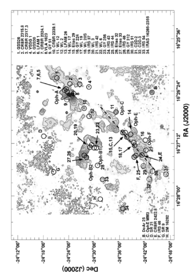
Figure 1: The L 1688 core in Ophiuchus. In grey-scale and contours the 850 $\mu$m SCUBA map as published by Johnstone et al. (2000) and Di Francesco et al. (2008) is shown. The locations of all the sources as observed in this study are shown, except for C2D-162527.6, Haro 1-4, C2D-162748.2 and IRS 63. C2D-16274.1 is marked as C2D-2 and C2D-162748.2 as C2D-3. The dashed line indicates the Oph ridge.

Table 1: Sample of embedded sources in L 1688, with additional known disks included.

Source	Other names	Coordinates (J2000)		Ref.a	$\alpha_{\rm{2-24\mu m}}$b
		RA	Dec
C2D-162527.6	SSTc2d J162527.6-243648	16:25:27.6	-24:36:48.4	2	0.36
GSS 26		16:26:10.4	-24:20:58	1	-0.46
CRBR 2315.8-1700		16:26:17.2	-24:23:45.1	2	0.69
CRBR 2317.3-1925.3	SKS 1-10	16:26:18.8	-24:26:13	1	-0.56
VSSG 1	Elias 20	16:26:18.9	-24:28:22	1	-0.73
GSS 30	Elias 21/GY 6/GSS 30-IRS1	16:26:21.4	-24:23:04.1	2	1.46
LFAM 1	GSS 30-IRS3	16:26:21.7	-24 22 51.4	2	0.73
CRBR 2324.1-1619		16:26:25.5	-24:23:01.6	2	0.87
VLA 1623	VLA 1623.4-2418	16:26:26.4	-24:24:30.3	2	no
GY 51	VSSG 27	16:26:30.5	-24:22:59	1	0.05
CRBR 2339.1-2032	GY 91	16:26:40.5	-24:27:14.3	2	0.45
WL 12	GY 111	16:26:44.0	-24:34:48	1	2.49
WL 2	GY 128	16:26:48.6	-24:28:39	1	0.02
LFAM 26	CRBR 2403.7/GY 197	16:27:05.3	-24:36:29.8	2	1.27
WL 17	GY 205	16:27:07.0	-24:38:16.0	1	0.61
Elias 29	WL15/GY 214	16:27:09.6	-24:37:21.0	1	1.69
GY 224		16:27:11.4	-24:40:46	1	-0.05
WL 19	GY 227	16:27:11.9	-24:38:31.0	1	-0.43
WL 20S	GY 240	16:27:15.9	-24:38:46	1	2.75
IRS 37	GY 244	16:27:17.6	-24:28:58	1	0.25
WL 3	GY 249	16:27:19.3	-24:28:45	1	-0.03
IRS 42	GY 252	16:27:21.6	-24:41:42	1	-0.03
WL 6	GY 254	16:27:21.8	-24:29:55	1	0.72
GY 256		16:27:22.0	-24:29:39.9	2	-0.05
IRS 43	GY 265	16:27:27.1	-24:40:51	1	1.17
IRS 44	GY 269	16:27:28.3	-24:39:33.0	1	2.29
Elias 32	IRS 45/GY 273/VSSG 18	16:27:28.6	-24:27:19.8	2	-0.03
Elias 33	IRS 47/GY 279/VSSG 17	16:27:30.1	-24:27:43	1	-0.12
IRS 48	GY 304	16:27:37.2	-24:30:34	1	0.88
GY 312		16:27:38.9	-24:40:20.5	2	0.64
IRS 51	GY3 15	16:27:40.0	-24:43:13	1	-0.15
C2D-162741.6	SSTc2d J162741.6-244645	16:27:41.6	-24:46:44.6	2	0.32
C2D-162748.2	SSTc2d J162748.2-244225	16:27:48.2	-24:42:35.6	2	1.55
IRS 54	GY 378	16:27:51.7	-24:31:46.0	1	0.03
IRAS 16285-2355		16:28:21.6	-24:36:23.7	2	1.23
C2D-162857.9	SSTc2d J162857.9-244055	16:28:57.9	-24:40:54.9	2	0.67
IRS 63		16:31:35.7	-24:01:29.5	2	0.14
Known Disks
Haro 1-4	DoAr 16	16:25:10.5	-23:19:14.5	2	-0.89
DoAR 25	GY 17	16:26:24.0	-24:43:09.0	1	-1.12
OphE MM3		16:27:05.9	-24:37:08.2	2	-0.33
SR 21	Elias 30	16:27:10.2	-24:19:16.0	1	-0.79
CRBR 2422.8-3423.8	CRBR 85	16:27:24.8	-24:41:03.0	1	1.01
IRS 46	GY 274	16:27:29.7	-24:39:16.0	1	0.18
SR 9	IRS 52/Elias 34	16:27:40.5	-24:22:07.0	1	-1.07
2MASS 16282		16:28:13.7	-24:31:39.0	2	-1.55

^a References for positions : 1:Bontemps et al. (2001), 2: c2d delivery document
^b From Evans et al. (2009). See also $\S$ 5.5

The YSO population was first identified by Elias (1978), Wilking & Lada (1983), Wilking et al. (1989), Comeron et al. (1993) and Greene et al. (1994) using IR observations. With the arrival of (sub-)mm telescopes, VLA 1623 in L 1688 was identified as the first deeply embedded YSO (Wootten 1989, Loren et al. 1990, André et al. 1993). In more recent years, a large population of Class I and Class II sources has been found based on their IR spectral slopes, using space-based observatories such as the Infrared Space Observatory (ISO) (e.g. Liseau et al. 1999, Bontemps et al. 2001) and ground-based IR (e.g. Barsony et al. 1997; 2005). Most embedded sources in L 1688 are clustered around the filaments of the Oph-A, Oph-B2, Oph-E and Oph-F regions, while the Oph-C region only shows a single embedded source and Oph-D does not have any embedded YSO (Motte et al. 1998). In Oph-E and Oph-F most sources are lined up along a relatively small filament of material: for the purpose of this paper, we will adopt the name ‘Ophiuchus ridge’ for this region.

With the launch of the Spitzer Space Telescope, the Ophiuchus cloud was included in the guaranteed time (GTO) and the ‘cores to disks’ (c2d) Legacy program (Evans et al. 2003). Padgett et al. (2008) report on the results at 24, 70 and 160 $\mu$m using the MIPS instrument, revealing the emission from the large-scale structure at mid and far-IR wavelengths. Jørgensen et al. (2008) compared the results from the c2d program with the COMPLETE 850 $\mu$m SCUBA sub-millimeter dust mapping from Johnstone et al. (2000) and Ridge et al. (2006) to determine the association of YSOs with dense cores.

The stellar ages of the Class II and III sources in Ophiuchus were found to be 0.1–1 Myr based on stellar spectroscopy compared with evolutionary tracks, indicating a relatively young age for the total cloud (Greene & Meyer 1995, Luhman & Rieke 1999). The Star-Formation Efficiency (SFE) was recently calculated with Spitzer and SCUBA photometry to be of the order of 13% within the cores and 4% in the cloud as found by Evans et al. (2009) and Jørgensen et al. (2008), lower than previous determinations (Wilking & Lada 1983).

The relative timescales of the different phases are determined by the number of objects in each class of YSOs (e.g. Evans et al. 2009). Recent high resolution ground-based (near)-IR imaging show that some of the Class I sources in Ophiuchus are physically different from an embedded YSO, confusing these timescales determinations. For example, the Class I source CRBR 2422.8-3423 was found to be an extincted edge-on disk from near-IR imaging (Brandner et al. 2000, Pontoppidan et al. 2005). The source OphE MM3, classified as a starless core by Motte et al. (1998), was also shown to be a edge-on disk in the same study (Brandner et al. 2000). The source IRS 46 has no associated protostellar envelope and was re-classified based on Spitzer and sub-mm data as a disk (Lahuis et al. 2006) . Much of the reddening seen in the IR originates from the nearby envelope associated with IRS 44.

Foreground material can also heavily influence the identification and subsequent analysis of embedded sources (e.g., Luhman & Rieke 1999). An excellent example is provided by the Class I source Elias 29 in L 1688, which has two foreground layers in addition to the ridge of material in which the YSO is embedded (Boogert et al. 2002). Only a combination of molecular line emission at sub-millimeter and IR spectroscopy could constrain the protostellar envelope as well as the immediate environment around it (Boogert et al. 2000; 2002). Indeed, IR spectroscopy can be used as a complementary diagnostic and spectra of many of the YSOs in Ophiuchus have been taken, using ISO, Spitzer or groud-based telescopes (e.g. Alexander et al. 2003, Pontoppidan et al. 2003, Boogert et al. 2008). Ice absorption features such as the 3 $\mu$m H₂O and 15.2 $\mu$m CO₂ bands are usually associated with embedded sources whereas silicate emission at 10 and 20 $\mu$m is characteristic of Class II sources, but foreground absorption and edge-on disks can confuse this classification (Boogert et al. 2002, Pontoppidan et al. 2005).

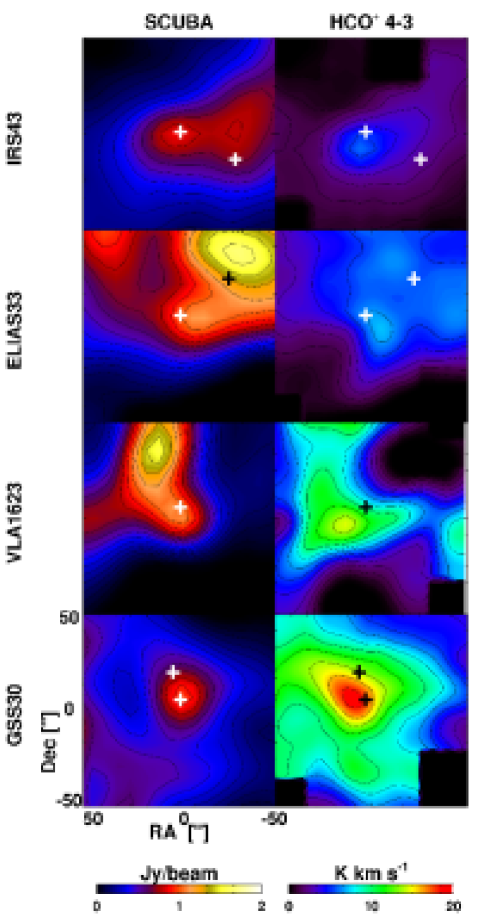
Figure 2: SCUBA 850 $\mu$m continuum (left) and HCO⁺ 4–3 (right) integrated intensity maps plotted from bottom to top for GSS 30 IRS1, VLA 1623, Elias 33 and IRS 43. The IR source positions are marked in the SCUBA maps with white crosses. Note that the absolute scale of these maps is a factor 4 higher than those in Fig. 3 and 4. The 850 $\mu$m continuum flux for VLA 1623 has been scaled down by a factor 4. In the map of GSS 30, LFAM 1 is located north of the GSS 30 IRS1 position. Elias 32 is located at the north-west side of the Elias 33 map. CRBR 2422.8-3423 is located to the south-west of IRS 43. All four main targets show strong HCO⁺ and SCUBA peaking within 5^′′ of the IR position at (0,0), characteristic of truly embedded sources.

In recent years, several detailed modelling efforts have been carried out to study the relations between the observed spectral energy distribution (SED) and the physical structure of embedded YSOs (e.g. Jørgensen et al. 2002, Whitney et al. 2003b, Schöier et al. 2004, Young et al. 2004, Robitaille et al. 2006; 2007, Crapsi et al. 2008). Whitney et al. (2003b) show that it is possible for embedded YSOs with a face-on projection to be classified as Class II. Due to their orientation, these sources are viewed straight down the outflow cone, directly onto the central star and disk system. Crapsi et al. (2008) show that a significant fraction of the Class I sources may be edge-on flaring disks, that have already lost their protostellar envelope. The spectral slope is much steeper than expected due to their structure.

A prime characteristic and component of embedded YSOs is the presence of dense centrally condensed envelopes. While dust maps at sub-millimeter wavelengths have become very popular to trace the early stages of star formation (e.g. Motte et al. 1998, Shirley et al. 2000, Johnstone et al. 2000, Stanke et al. 2006), the continuum emission at these wavelengths is dominated by the cold outer envelope and cloud material, with disks starting to contribute as the envelope disperses (e.g. Hogerheijde et al. 1997, Looney et al. 2000, Young et al. 2003). Single-dish dust continuum data by themselves are not able to distinguish between dense cores and envelope or foreground material, nor quantify any disk contributions. However, the dense gas ($\sim$10⁶ cm^-3) located in the inner regions of protostellar envelopes is uniquely probed by molecular lines with high critical densities at sub-millimeter wavelengths. Observations of deeply embedded Class 0 YSOs have indeed revealed strong sub-millimeter lines of various molecules (e.g. Blake et al. 1994; 1995, Schöier et al. 2002, Jørgensen 2004, Maret et al. 2004; 2005), but only a few studies have been carried out on more evolved Class I embedded YSOs (e.g. Hogerheijde et al. 1997).

A good high density tracer is the HCO⁺ molecule, for which the $J=$4–3 line both has a high critical density of $>$10⁶ cm^-3 and is accessible from the ground. Dense gas is also found in the circumstellar disk on scales of a few tens to hundreds AU, but such regions are generally diluted by an order of magnitude in single-dish observations. In contrast, molecular lines with much lower critical densities, such as the low excitation C¹⁸O transitions, contain much higher contributions from low density material. This makes these lines well-suited as column density tracers for large-scale cloud material and the cold outer regions of the protostellar envelope (e.g. Jørgensen et al. 2002). Both the HCO⁺ and C¹⁸O data have velocity resolutions of 0.1 km s^-1 or better, thus allowing foreground clouds to be identified.

Most sub-millimeter line data so far have been single pixel spectra toward the YSO with at best a few positions around specific YSOs. The recently commissioned HARP-B instrument is a 16-pixel receiver, operating in the 320 to 370 GHz atmospheric window allowing rapid mapping of small (2^′) regions (Smith et al. 2003). HARP-B is mounted on the James Clerk Maxwell Telescope (JCMT).

We present here HARP-B maps of all Class I sources in the L 1688 region in C¹⁸O 3–2 and HCO⁺ 4–3. The combination of these two molecular lines allows us to differentiate between protostellar envelopes, dense cores and foreground cloud material, as well as edge-on disks. The goal of this paper is to characterize the envelopes of the embedded source population of L 1688, as well as present a new method for identifying truly embedded sources and separate them from (obscured) edge-on disks using the dense gas present in embedded YSOs. In $\S$ 2, a sample of Class I sources in the L 1688 core is selected. In $\S$ 3, we discuss the details of the heterodyne observations carried out at the JCMT and the Atacama Pathfinder EXperiment (APEX), as well as the supplementary observations obtained in a continuum i.e. wideband mode. $\S$ 4 presents the maps and spectra and in $\S$ 5 we analyze the properties of the gas and dust of the sources in the sample. The environment around the YSOs, column density, envelope gas and concentration of the HCO⁺ are discussed. In $\S$ 6, we present a new method for identifying embedded YSOs from (edge-on) disks and apply this method to the sample. This classification is then compared to traditional methods as well as other recently proposed methods. The main conclusions of the paper are given in $\S$ 7.

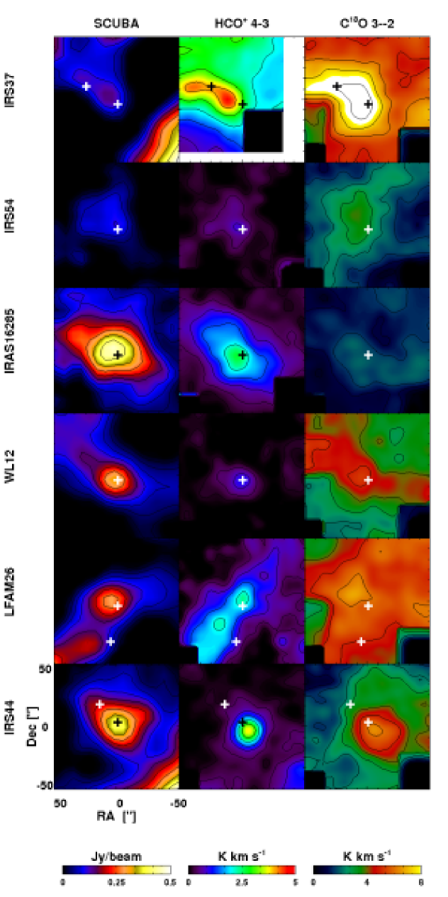
Figure 3: SCUBA 850 $\mu$m continuum (left), HCO⁺ 4–3 (middle) and C¹⁸O 3–2 (right) integrated intensity maps plotted for (from bottom to top) IRS 44, LFAM 26, WL 12, IRAS 16285, IRS 54 and IRS 37. The locations of the IR sources are indicated in the SCUBA maps with white crosses. In the IRS 44 map, IRS 44 is indicated with a black cross, and IRS 46 with a white one. In the LFAM 26 field, OphE MM3 is located south of LFAM 26. In the IRS 37 field, WL 3 is located west of IRS 37. The sources at (0,0) in this figure show weaker HCO⁺ images than in Fig. 2, but are still peaking on the IR positions in both SCUBA and HCO⁺, and are thus embedded YSOs according to our classification.

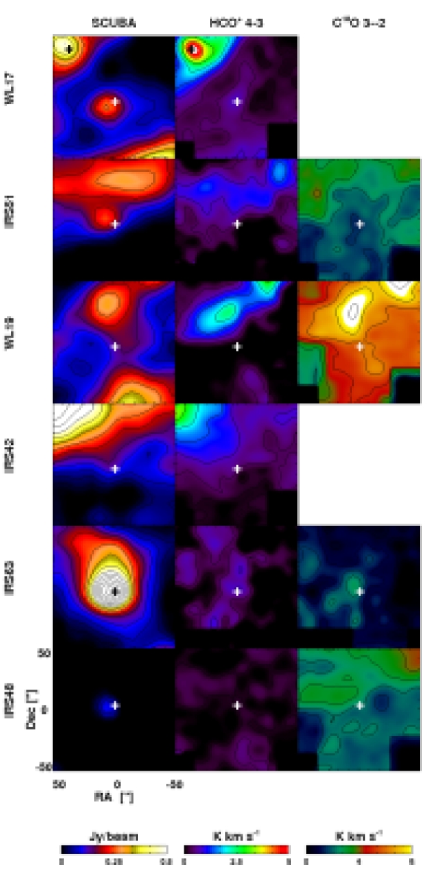
Figure 4: SCUBA 850 $\mu$m continuum (left), HCO⁺ 4–3 (middle) and C¹⁸O 3–2 (right) plotted for (from bottom to top) IRS 48, IRS 63, IRS 42, WL 19, IRS 51 and WL17. The locations of the IR sources are indicated in the SCUBA maps with white crosses. The embedded source Elias 29 is shown with a black cross in the field of WL 17. The peak 850 $\mu$m flux density for IRS 63 is 1.1 Jy beam^-1; it was not scaled to accentuate the extended dust emission. The sources at (0,0) in this image are mostly unresolved in SCUBA and show little or no HCO⁺ emission related to the source. They are either transitional or confused sources or (edge-on) disks in our new classidfication, with the exception of IRS 63, which is classified as embedded (transitional).

2 Sample Selection

Of the known (embedded) YSO population within L 1688, 45 objects were selected for our sample using several criteria. First, we require all sources be located within the 850 $\mu$m dust continuum map made by the COMPLETE project of L 1688 using SCUBA on the JCMT (Johnstone et al. 2000).

Second, sources must be included in the area covered by the c2d program using IRAC and MIPS on Spitzer (Evans et al. 2003, Padgett et al. 2008). All sources classified as Class I in either André & Montmerle (1994), Barsony et al. (1997), Bontemps et al. (2001) or the c2d delivery document (Evans et al. 2007) are included with luminosities $>$ 0.04 L_⊙. Although these 41 objects have been classified as Class I in one or more of these papers, only 6 of these have been classified consistently as Class I in all studies. Most other sources are classified as either Class II or Flat spectrum sources at least once. All such sources are included in the analysis of this paper, but conversely, our sample does not include all Flat spectrum or Class II sources listed in the c2d survey. Known edge-on disks such as 2MASS 16282, IRS 46, OphE MM3 and CRBR 2422.2-3423, are among these 41 sources and are included within the sample to illustrate the results of our method for such sources. The sample should not contain any reddened background main-sequence stars which are readily identified in the c2d analysis. However, other background sources, such as AGB stars or background infrared galaxies, may be present.

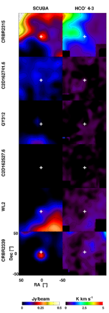
Figure 5: SCUBA 850 $\mu$m continuum (left) and HCO⁺ 4–3 (right) plotted for (from bottom to top) CRBR 2339.1, WL 2, C2D 162527.6, GY 312, C2D 162741.6 and CRBR 2315.8. The locations of the sources are indicated in the SCUBA maps with white crosses. These sources have either unresolved or little or no emission in the SCUBA 850 $\mu$m and HCO⁺ 4–3 maps at (0,0), making them disk sources in our classification.

Four sources with $\alpha_{\rm{2-24\mu m}}$$>$ 0.0 were found only in the recent Spitzer observations. These are SSTc2d J162527.6-243648, SSTc2d J162741.6-244645, SSTc2d J162748.2-244225 and SSTc2d J162857.9-24405. The names C2D-162527.6, C2D-162741.6 , C2D-162748.2 and C2D-162857.9 are adopted. VLA 1623-2418 is included as an embedded Class 0, but it is generally absent from the above studies. In addition, IRS 63 was included, although it is not part of the L 1688 core, due to its interesting characteristics as a Class I source as observed with the SubMillimeter Array (SMA). These recent interferometric results suggest that this source is an embedded YSO with little envelope material left, and, as such, presents an interesting test case for the proposed method of identifying truly embedded sources (Lommen et al. 2008). Four disk sources within or near to the L 1688 region, Haro 1-4, DoAr 25, SR 9 and SR 21, were included to serve as a sample of known disk sources.

The final source sample, which covers all potential Class I sources, can be found in Table 1. The positions as found in Bontemps et al. (2001) were used where available. If the source was not included in Bontemps et al. (2001), or if confusion exists due to nearby IR sources, the position as found in the c2d delivery document (Evans et al. 2007) was adopted. For sources in common, most positions agree within 3^′′. Fig. 1 shows the distribution of the sample as plotted on the SCUBA 850 $\mu$m map of L 1688 (Johnstone et al. 2000, Ridge et al. 2006, Di Francesco et al. 2008).

Figure 6: HCO⁺ 4–3 spectra extracted from the HARP-B maps in a 15^′′ around the IR positions. Sources classified as embedded in $\S$ 6.2 are shown in the left column. In the right column, the sources classified as confused or disks are plotted.

The table includes the spectral index $\alpha_{\rm{2-24\mu m}}$ given in Evans et al. (2009), calculated from the 2MASS, IRAC and MIPS (24 $\mu$m only) fluxes. No $\alpha_{\rm{IR}}$ could be determined from Spitzer data for VLA 1623 (too faint)

3 Observations

3.1 Gas line maps

The majority of the sample was observed in HCO⁺ 4–3 (356.7341 GHz) and C¹⁸O 3–2 (329.3305 GHz) using the recently commissioned 16-pixel heterodyne array receiver HARP-B on the James Clerk Maxwell Telescope (JCMT). The high spectral resolution mode of 0.05 km s^-1 available with the ACSIS back-end was used to disentangle foreground material as well as any contributions from outflowing material. Spectra were subsequently binned to 0.15 km s^-1.

HARP-B observations of 30 sources in 21 fields were carried out during July and August 2007 in C¹⁸O 3–2 and HCO⁺ 4–3 under weather conditions with an atmospheric optical depth, $\tau_{225\rm{GHz}}$ ranging from 0.035 to 0.08 (precipitable water vapor of 0.7 to 1.6 mm). The fields were observed down to a rms noise of 0.1 K in a 0.5 km s^-1 bin. The HARP-B pixels have typical single side-band system temperatures of 300–350 K. The 16 receivers are arranged in a 4$\times$4 pattern, separated by 30^′′. This gives a total foot print of 2^′ with a spatial resolution of 15^′′, the beam of the JCMT at 345 GHz. The 2${}^{\prime}\times 2^{\prime}$ fields were mapped using the specifically designed jiggle mode HARP4. A position switch of typically 30^′ in azimuth was used, with larger throws if needed. The Class 0 source IRAS 16293-2422 was used as a line calibrator and pointing source. Calibration errors are expected to dominate the flux uncertainties, and are estimated at 20$\%$. Pointing was checked every two hours and was generally found to be within 2–3^′′. The map was re-sampled with a pixel size of 5^′′, which is significantly larger than the pointing error. The main-beam efficiency was taken to be 0.67. Data were reduced using the STARLINK package GAIA and the CLASS reduction package.

3.2 Gas single pixel spectra

Supplementary data of HCO⁺ 4–3 were taken at the APEX telescope during July 2007, using the APEX-2a receiver. All sources were observed for which no HARP-B data were taken, except GSS 26 and GY 51. The APEX observations were done in excellent weather conditions with $\tau_{225\rm{GHz}}$ ranging from 0.01 to 0.04 (PWV 0.2 to 0.8 mm). Single spectra were taken with a spectral resolution of 0.4 km s^-1 down to an rms of 0.3 K. Calibration errors are estimated to be $\sim 20$%. The APEX 12-m dish is slightly smaller than the JCMT 15-m dish, producing a beam of 18^′′ instead of 15^′′. Pointing errors are $<$4^′′. Beam efficiency is 0.70.

For the sources GSS 30, VLA 1623, WL 20S, IRS 42, IRS 43, Elias 32 and Elias 33, C¹⁸O 3–2 spectra were obtained from the CADC archive. These spectra were taken with the RxB receiver during September 2005.

Figure 7: C¹⁸O 3–2 spectra extracted from the HARP-B maps at the source positions. Spectra are arranged in random order to illustrate the independence of C¹⁸O to the environment instead of the protostellar envelope.

Table 2: Results from HARP-B (HCO⁺ 4–3 and C¹⁸O 3-2), APEX-2a (HCO⁺ 4–3) and RxB (C¹⁸O 3–2) observations at the source position.

Source	HCO+ 4-3a		C18O 3–2		Notes
	$\int$ $T_{\rm{MB}}$ dV	$T_{\rm{MB}}$	$\int$ $T_{\rm{MB}}$ dV	$T_{\rm{MB}}$
	[K km s-1]	[K]	[K km s-1]	[K]
C2D-162527.6	-	$<$0.09	-	-	See Fig. 5
GSS 26	-	-	-	-	See Fig. 9
CRBR 2315.8-1700	6.3	5.2*	-	-	See Fig.5
CRBR 2317.3-1925	1.5b	2.0b	-	-	See Fig. 9
VSSG 1	-	$<$0.4	-	-	See Fig. 9
GSS 30	16.7	9.1	10.7c	6.3c	See Fig.2 and 10
LFAM 1	18.4	10.8	-	-	See Fig.2 and 10, GSS 30 maps
CRBR 2324.1-1619	-	-	14.5	12.2	See Fig.2 and 10, VLA1623 maps
VLA 1623	16.2	9.0	10.4	17.9d	See Fig.2 and 10
GY51	-	-	-	-	See Fig. 9
CRBR 2339.1-2032	0.55	0.45*	-	-	See Fig.5
WL 12	0.87	1.4	4.8	3.9	See Fig.3 and 10
WL 2	0.3	0.18*	-	-	See Fig.5
LFAM 26	1.95	1.8	6.4	3.3	See Fig.3
WL 17	0.6	0.45	-	-	See Fig.4
Elias 29	4.5b	2b	10.4e	4.3e	See Fig.4, WL17 map and Fig. 9 and 10
GY 224	-	$<$0.27b	-	-	See Fig. 9
WL19	-	$<$ 0.1	6.3	4.5	See Fig.4
WL 20S	-	$<$0.26b	5.0c	2.3c	See Fig. 10
IRS 37	3.7	2.5	9.55	5.7	See Fig.3
WL 3	3.7	2.2	8.8	6.3	See Fig.3, IRS 37 map
IRS 42	0.45	0.7*	4.0	1.2*	See Fig.4
WL 6	0.92	0.6	5.25	4.5*	See Fig. 9 and 10
GY 256	0.75	0.45*	5.4	4.5*	See Fig. 9 and 10, WL6 maps
IRS 43	4.5d	1.6d	6.5c	3.2c	See Fig. 2,9 and 10
IRS 44	3.4d	0.5d	5.8	2.8	See Fig.3
Elias 32	5.6	4.3	3.1c	4.5c	See Fig.2 and 10, Elias 33 maps
Elias 33	6.3	5.7	6.0c	3.0c	See Fig.2 and 10
IRS 48	-	$<$0.09	2.6	2.3	See Fig.4
GY 312	-	$<$0.1	-	-	See Fig.5
IRS 51	0.75	0.75	2.0	2.8*	See Fig.4 and 10
C2D-162741.6	-	$<$ 0.1	-	-	See Fig.5
C2D-162748.1	-	$<$ 0.34b	-	-	See Fig. 9
IRS 54	0.53	0.45	3.4	3.3	See Fig.3
IRAS 16285-2355	2.1	3.0	2.3	3.0	See Fig.3
C2D-162857.9	-	$<$ 0.34b	-	-	See Fig. 9
IRS 63	0.75	1.2	1.7	3.3	See Fig.4
Disks
Haro 1-4	-	$<$0.29b	-	-	See Fig. 9
DoAR 25	-	$<$0.28b	-	-	See Fig. 9
OphE MM3	1.7	1.6*	5.5	3.0*	See Fig.3, LFAM 26 map
SR 21	-	$<$0.28b	-	-	See Fig. 9
CRBR 2422.8-3423	1.9	1.4*	-	-	See Fig. 2, IRS 43 map, and Fig.4,NW corner of IRS 42
IRS 46	-	$<$0.09	2.9	2.1	See Fig.3, IRS 44 map
SR 9	-	$<$0.24b	-	-	See Fig. 9
2Mass 16282	-	$<$0.35b	-	-	See Fig. 9 and 10

^a Intensities marked with a * do not peak at source position
^b APEX-2a receiver. Upper limits (2$\sigma$) in 0.4 km s^-1 bin
^c JCMT RxB data
^d Outflowing gas detected (width $\sim$20 km s^-1)
^e C¹⁸O data taken from Boogert et al. (2002), obtained with the CSO.

Figure 8: HCO⁺ 4–3 spectra at the source positions obtained at APEX. Elias 29 and IRS 43, with clear detections, are the only sources found to be embedded in $\S$ 6.2. The detection seen for CRBR 2317 is attributed to the cloud material and is classified as a disk.

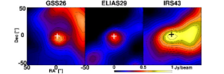
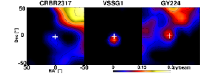
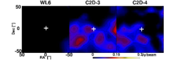
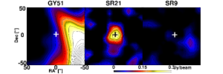
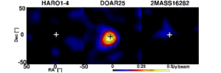
Figure 9: Dust maps at 850 $\mu$m extracted from the JCMT-SCUBA COMPLETE map of GSS 26, Elias 29 and IRS 43; CRBR 2317.3-1925, VSSG 1 and GY 224; WL 6, C2D-162748.2 (C2D-3) and C2D-162857.9 (C2D-4); GY 51, SR 21 and SR 9; Haro 1-4, DoAr 25 and 2MASS 16282. Note that the emission toward GY 51 is scaled down by a factor of 4.

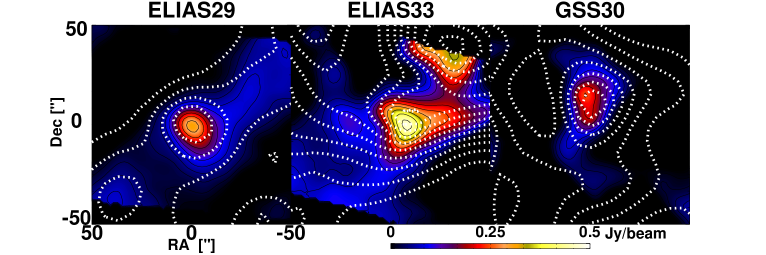
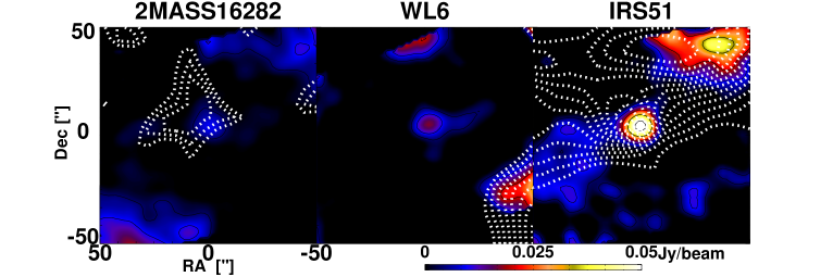
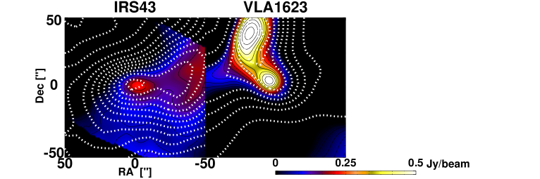
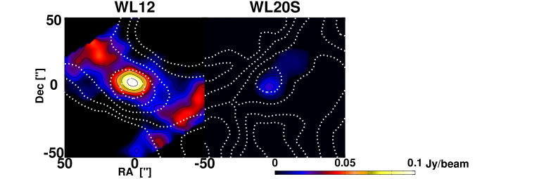
Figure 10: Dust maps at 350 $\mu$m observed with the SHARC-II instrument at the CSO. In white, the contours for the JCMT-SCUBA 850 $\mu$m data are over-plotted, normalized for the maximum emission in the map in contours of 10$\%$, 30$\%$, 50$\%$ and 70 $\%$. The shape of the contour levels at 850 $\mu$m agrees well with those found at 350$\mu$m.

3.3 Dust maps

The 850 $\mu$m continuum data of the Ophiuchus region, obtained within the scope of the COMPLETE project using the SCUBA instrument on the JCMT, were used to characterize the dust in the environments around all sources of the sample (Johnstone et al. 2000, Ridge et al. 2006, Di Francesco et al. 2008). The most recent map, version 3, was used to extract the information (see Fig. 1). This version includes a correction for the chopped out-emission. Integrated fluxes within regions with radii ranging from 25^′′ to 40^′′ were extracted from the map (see Table 9). The exact radii were selected by calculating the FWHM to the peak flux of each source. Comparison with the map and published fluxes by Johnstone et al. (2000) within similar radii found by a clumpfind routine showed that fluxes agreed within 5$\%$, significantly better than the calibration error of 20$\%$ for SCUBA. The sensitivity of the SCUBA map is such that sources down to 90 mJy (3$\sigma$) can be detected.

In addition, 11 sources were observed using the SHARC-II 350 $\mu$m continuum instrument at the Caltech Submillimeter Observatory (CSO) during April 2003 (Dowell et al. 2003). The array has 12$\times 32$ pixels, spanning 4.85^′′ per pixel, which results in a footprint of 1${}^{\prime}\times 2.6^{\prime}$ and a beam size of $9^{\prime\prime}$. The sources observed with the CSO were GSS 30, WL 12, Elias 29, VLA 1623, OphE MM3, WL 20S, WL 6, IRS 43, VSSG 17, IRS 51, 2MASS 16282. The data were reduced with the CRUSH package and calibrated using observations of Mars and Saturn. If no planets were available during the specific night, IRAS 16293-2422 was used to calibrate the data. The calibration errors are estimated to be on the order of 30–40$\%$ and assumed to dominate the error in the flux estimate over other instrumental errors or $S/N$ considerations. The sensivity of the SHARC-II maps is such that sources down to 400 mJy (3$\sigma$) can be detected. For a typical dust flux law $\propto\nu^{3.5}$, this implies that the SHARC-II data are a factor of 4 more sensitive to low-mass sources than the SCUBA data.

3.4 SED and IRS spectra

The L 1688 core has been targeted by a large number of continuum surveys, covering wavelengths from 2 to 1300 $\mu$m. 2MASS (1.25, 1.66 and 2.2 $\mu$m) and Spitzer-IRAC (3.6, 4.5, 5.8 and 8 $\mu$m) and Spitzer-MIPS (24 $\mu$m) fluxes were obtained from the c2d delivery document (Evans et al. 2007). Recently, Padgett et al. (2008) presented Spitzer-MIPS 70 and 160 $\mu$m fluxes. The MIPS 160 $\mu$m data were not used in our analysis since a large part of the map was confused by either striping or saturation. For the MIPS 70 $\mu$m data, we chose to go back to the original data and retrieve the 70 $\mu$m fluxes source-by-source in a typical 10^′′ radius using PSF photometry without the extended contribution subtracted. This avoids potential errors in the flux estimates from automatic extraction in crowded or confused regions such as the Ophiuchus core. In addition to the SCUBA (850 $\mu$m) and/or SHARC-II (350 $\mu$m) fluxes, a limited number of sources was also observed using SHARC-II and/or SCUBA at 450 $\mu$m in a recent survey of disks in the L 1688 core, with fluxes given in the central 15^′′ beam (Andrews & Williams 2007). Where available, archival data at millimeter wavelengths were used from SEST and IRAM 30m, as reported in Andrews & Williams (2007) and originally obtained by André & Montmerle (1994), Jensen et al. (1996), Nuernberger et al. (1998), Motte et al. (1998) and Stanke et al. (2006).

A number of sources in our sample have also been observed with various observing programs using the IRS instrument on Spitzer at 5-40 $\mu$m (PID= 2, 172 and 179). These spectra are included in this study to confirm the continuum fluxes in the wavelength range of IRS, and to investigate the presence of ice absorption and silicate absorption or emission.

4 Results

4.1 Gas maps

Fig. 2 to 5 present the 21 observed HARP-B fields for HCO⁺ 4–3 and C¹⁸O 3–2, together with the SCUBA 850 $\mu$m continuum map. Note that the sources in Fig. 2 are much brighter and have different intensity scales. The integrated intensity and peak temperatures for all sources are listed in Table 2, columns 2 to 5. Column 7 states in which figure(s) the sources are mapped or in which figure(s) its spectra are plotted. Fig. 6 (HCO⁺) and 7 (C¹⁸O) show spectra extracted from the maps at the positions of the sources. About 70$\%$ of the sample was observed in C¹⁸O 3–2. The sources for which APEX-2a HCO⁺ spectra were taken can be found in Fig. 8.

Using the molecular line emission maps, the sample can be divided roughly into three groups. In the first (see Fig. 2 and 3), HCO⁺ peaks at or close to the source positions, with peak intenstities up to a few K. For these sources, GSS 30 IRS1, LFAM 1, VLA 1623, WL 12, LFAM 26, IRS 37, WL 3, WL 17, Elias 33, Elias 32, IRS 44, IRAS 16285 and IRS 54, HCO⁺ seems to be extended on scales of a few 10^′′. C¹⁸O is always present in these maps, and also extended on scales of a few 10^′′ to 1^′.

Note that the HCO⁺ maps in some case show minor offsets w.r.t. the IR positions. For offsets $<$ 8^′′ this can be attributed to either the pointing accuracy of the JCMT or the differences between IR positions from Bontemps et al. (2001) and c2d. For a few sources, in particular VLA 1623, IRS 44, larger offsets up to 12^′′ were found. These can be accounted for by potentially three effects. First, self-absorption of HCO⁺. Second, these sources show strong outflow emission, which peaks off-source and significantly influences the spectrally integrated maps. Third, molecular emission can be suppressed by the freeze-out of molecules in the cold part of the cloud.

A second group (Fig. 4 and 5) lacks detections in HCO⁺, down to a limit 0.1 K. The sources, C2D-162527.6, WL 19, IRS 46, IRS 48, GY 312 and C2D-162741.6 belong to this group. The third group (Fig. 4 and 5) of sources contains CRBR 2315.8-1700, CRBR 2339.1-2032, WL 2, OphE MM3, IRS 51 and IRS 42. These show HCO⁺ detections at the source position. The HCO⁺ is extended, but there is no sign of a peak at the source positions. For IRS 63 and WL 6, detections of HCO⁺ are marginal at $\sim$3 $\sigma$.

The HCO⁺ 4–3 integrated intensities $\int T_{\rm{MB}}$dV in protostellar envelopes range from as high as 18.4 K km s^-1 for LFAM 1 to 0.75 K km s^-1 for IRS 63. In $\S$ 5.3 the HCO⁺ 4–3 integrated intensities are compared with the column densities derived from the C¹⁸O 3–2. This shows that most embedded sources with strong HCO⁺ emission are located in regions with high column densities. The sole exception is IRAS 16285-2355, which is not located in a region with high column density (see Fig. 1 and 3). However, it is possible to find sources with little or no HCO⁺ 4–3 emission, such as WL 19, in regions with similarly high column density.

4.2 Dust maps

For sources for which molecular emission was taken with the HARP-B array, the spatial extent of the dust is shown in the left column in Fig. 2-5. The sources for which no HARP-B maps were obtained can be found in Fig. 9. The SHARC-II maps are shown in Fig. 10. In these maps, the white contours show the 850 SCUBA emission. The integrated fluxes in a 25^′′ beam are given in Tables 3 and 9.

Table 3: Source fluxes at 350 $\mu$m in a 25^′′ beam observed with SHARC-II at the CSO.

Source	Flux	Concentrationa
	(Jy)
GSS 30	2.5	0.58
WL12	6.7	0.59
Elias 29	4.3	0.72
VLA1623	40	0.8
WL20S	0.82	0.64
WL6	$<$0.4	U
IRS 43	2.1	0.62
Elias 33	4.4	0.55
IRS 51	1.4	0.64
2MASS 16282	$<$0.2	U

^a See $\S$5.1; U=not determined since only flux upper limits obtained.

Both the SHARC-II and SCUBA images clearly show that the dust is extended on scales of at least a few arcminutes at many positions in Ophiuchus. The smaller beam and higher frequency of the SHARC-II observations is able to both resolve smaller envelopes (e.g., Elias 33) or confirm that other sources (e.g., WL 20S) are not resolved at 350 $\mu$m down to 9^′′. The extended emission originates from cold dust in the parental cloud, as mapped by Motte et al. (1998), Johnstone et al. (2000) and Stanke et al. (2006). This cloud material can exist close to or in the line of sight of many of the Class I sources, but is not necessarily associated with a protostellar envelope, as is often assumed. A good example is the source WL 19 (Fig. 4), where dust emission is found close to the position of the source, but does not peak at the position of WL 19. This emission comes from a prestellar core within the Ophiuchus ridge and not a protostellar envelope.

Based on the spatial extent of the dust, the sample can be divided into four groups. First there are sources with spatially extended dust emission profiles, peaking at the source position. Examples are GSS 30 IRS1, Elias 29 and IRS 43. A second group shows extended dust emission, but with no central peak at the position of the source. A good example is GY 51 (see Fig. 9), located close to the Oph-A core. Some Class I sources only show unresolved dust emission at the source position, such as IRS 51 (see Fig.10). A final group shows no emission at 350 or 850 $\mu$m down to our sensitivity limits. Good examples is Haro 1-4.

Cloud material can contribute significantly or even dominate the emission on the scales probed by SCUBA and SHARC-II. Two fluxes at 850 $\mu$m are therefore given in Table 9. The first flux is within the 15^′′ beam obtained from Andrews & Williams (2007). If no value was given by them, it was extracted from the COMPLETE map for the central beam. Our extracted fluxes agree to within 15% for sources also listed in Andrews & Williams (2007), even though we include estimates to reconstruct the chopped-out extended emission. The second flux is extracted from the COMPLETE map for larger apertures encompassing the envelopes, up to a 25^′′ ($\sim$3,000 AU) radius, the typical envelope extent where the temperature and density drop to that of the surrounding cloud. The first number should thus be considered a lower limit on the total envelope and disk emission, while the second is an equivalent upper limit. For disk sources, all emission originating from the source is located within 15^′′ ($<$1,800 AU).

4.3 SED and IRS spectra

Table 9 summarizes all the Spitzer and (sub-)millimeter fluxes. The 2 $\mu$m to 1.3 mm flux densities for all 45 sources are plotted in Fig. 11. In addition, low-resolution IRS spectra are over-plotted between $\sim$5-30 $\mu$m, where available. In the on-line appendix, blow-ups of the IRS spectra are presented.

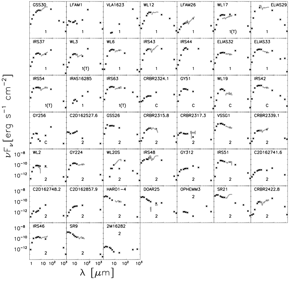
Figure 11: The spectral energy distributions of all sources, supplemented by spectra taken with IRS. Our classification can be found near the center and bottom of each SED. 1 = Embedded Stage 1, 1(T) = Transitional from embedded to pre-main sequence, C = confused and 2 = (edge-on) disk.

Table 4: Source properties derived from the gas and dust. The table has been rearranged compared with Table 1 to reflect the classification in $\S$6.2

Source	$\alpha_{\rm{IR}}$	$N_{\rm{H}_{2}}^{a}$	$\Delta\alpha^{b}$	Massc	$L_{\rm{bol}}$	$T_{\rm{bol}}$	$C_{850}$d	$C_{\rm{HCO^{+}}}$d
		(1022 cm${}^{-2})$		(10-2 $M_{\rm{\odot}})$	(10-1 L⊙)	(K)
Embedded sources
GSS 30e	1.46	23.3/19.4*	2.6	20.5	33	123	0.55	0.69
LFAM 1e	0.73	50*	2.6	17.1	8.3	86	0.59	0.69
VLA 1623	no	441*	-	111	2.7	12	0.7	0.72
WL 12	2.49	10.5/15.2*	3.1	4.6	34	155	0.26	0.81
LFAM 26	1.27	14.0/18.5*	4.4	4.5	0.44	238	0.40	0.69
WL 17	0.61	8.4*	1.0	4.0	6.7	323	0.22	0.71
Elias 29	1.69	22.7/33.6*	1.5	6.2	25	424	0.49	-f
IRS 37e	0.25	20.8	1.0	1.2	3.8	243	0.58	0.72
WL 3e	-0.03	19.2/9.7*	2.3	2.9	4.6	192	0.25	0.67
WL 6	0.72	11.4	-	$<$0.4	8.5	394	U	0.77
IRS 43	1.17	14.2/20.7*	2.3	17.1	10	134	0.58	0.79
IRS 44	2.29	12.6/30.2D*	2.9	8.0	11	140	0.33	0.80
Elias 32	-0.03	6.8/140*	3.7	41.9	5	321	0.37	0.70
Elias 33	-0.12	13.1/96*	3.1	28.2	12	460	0.6	0.64
IRS 54	0.03	7.4	1.2	3.1	7.8	486	0.8	0.80
IRAS 16285-2355	1.23	5.0/41.9D*	3.1	10.3	0.57	77	0.45	0.80
IRS 63	0.14	3.7/84.0D*	-	16.4	13	363	0.75	0.60
Confused sources
CRBR 2324.1-1619	0.87	31.6/70.5*	5.2	39.3	0.44	283	U	U
GY51	0.05	27.7*	4.5	11.1	2.3	706	U	U
WL19	-0.43	13.7/16.8*	4.9	5.5	1.5	730	0.15	0.53
IRS 42	-0.03	8.7/14.2*	1.3	4.7	14	540	0.44	0.60
GY 256	-0.05	11.8	-	$<$0.2	1.1	104	U	0.70
Disks
C2D-162527.6	0.36	-	-	$<$0.4	0.16	1051	U	U
GSS 26	-0.46	24.3D*	1.8	10.2	3.2	877	0.65	U
CRBR 2315.8-1700	0.69	17.6*	1.0	5.1	0.93	456	0.38	0.74
CRBR 2317.3-1925	-0.56	12.6*	0.3	1.1	0.11	1105	0.85	S
VSSG 1	-0.73	20.1*	-	2.0	5.8	930	0.74	SU
CRBR 2339.1-2032	0.45	6.7*	-	2.0	0.55	426	0.55	0.58
WL 2	0.02	-	-	1.0	0.88	573	0.3	0.58
GY 224	-0.05	10.9*	1.0	2.4	2.1	614	0.63	SU
WL 20S	2.75	10.9/15.3D*	1.0	3.9	4.5	85	0.57	SU
IRS 48	0.88	5.7/15.2D*	2.1	1.2	81	238	0.70	U
GY 312	0.64	-	-	$<$0.2	0.73	285	U	0.3
IRS 51	-0.15	4.4/18.4D*	2.3	5.0	8	548	0.27	0.59
C2D-162741.6	0.32	-	-	2.3	0.28	279	U	U
C2D-162748.2	1.55	-	-	0.4	0.17	241	U	SU
C2D-162857.9	0.67	-	-	5.6	0.22	402	U	SU
Haro 1-4	-0.89	-	-	0.45	5.6	762	U	SU
DoAR 25	-1.12	38.6*	-	3.4	4.7	1422	0.90	SU
OphE MM3	-0.33	12.0/13.4*	3.4	2.3	0.17	45	U	0.68
SR 21	-0.79	33.6*	-	3.1	1.8	1070	0.89	SU
CRBR 2422.8-3423	1.01	106.6*	2.3	20.5	4.4	157	U	-f
IRS 46	0.18	6.3/15.1*	2.8	3.3	1.9	684	U	SU
SR 9	-1.07	-	-	$<$0.4	8.7	1588	U	SU
2MASS 16282	-1.55	-	-	1.7	0.84	66	U	SU

^a Column densities marked with * are calculated from the SCUBA dust maps. Embedded sources where a large disk contribution is likely are indicated with a D. Note that no column densities could be calculated from the dust below 1$\times 10^{23}$ cm^-2 .
^b $\Delta\alpha$ is an upper limit to change in 2-24 $\mu$m spectral slope due to the reddening by foreground clouds at this source. This is derived by considering the mean column density at 45^′′ off the source position.
^c Upper limit derived from the 850 $\mu$m data using the relation from Shirley et al. (2000), with the assumption that all 850 $\mu$m emission originates within a protostellar envelope.
^d U=Undetected or Unobserved, S=single position spectrum available only
^e Circumbinary envelope.
^f Although both Elias 29 and CRBR 2422.8-3423 were observed, these sources are located near the edge of a field and do not have sufficient coverage to obtain a concentration parameter for the HCO⁺.

5 Analysis

5.1 Concentration

One method to distinguish embedded YSOs from edge-on disks, starless cores or background sources such as AGB stars and galaxies, is to use a measure of how centrally concentrated the emission is. This method has been used previously in the analysis of SCUBA data (Johnstone et al. 2001, Walawender et al. 2005, Jørgensen et al. 2007) by defining a concentration parameter:

$$C=1-\frac{1.13B^{2}S_{850}}{\pi R^{2}_{\rm{obs}}F_{0}}$$ (1)

where $B$ is the beam-size, $S_{850}$ is the total flux at 850 $\mu$m within the envelope, $R^{2}_{\rm{obs}}$ is the observed radius of the envelope and $F_{0}$ is the peak flux of the envelope. The observed radii were selected by calculating the FWHM to the peak flux of each source. The level of concentration potentially provides an indication of the evolutionary stage. Highly concentrated cores ($C>$ 0.75) have a very high probability to contain protostars, while cores with low concentration ($C<$ 0.4) are often starless, as indicated by the absence of near-IR emission. The observed radii in the 850 $\mu$m maps were defined by Kirk et al. (2006) as $R=(A/\pi)^{1/2}$, with A the area of the core within the lowest contour of their clumpfind routine. The SHARC-II maps also allow a concentration at 350 $\mu$m to be made, as seen in Table 3. These concentrations are found to be within 10$\%$ to those found for the 850 $\mu$m data, with the exception of WL12 which is more than a factor 2 higher in the SHARC-II 350 $\mu$m data.

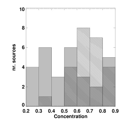
Figure 12: The distribution of concentration of SCUBA (gray) and HCO⁺ 4–3 (striped). Only sources with spatially resolved profiles have been taken into account. Note that the total number of sources is greater for SCUBA than for HCO⁺.

A similar concentration parameter can also be calculated for the distribution of HCO⁺, using integrated intensities between $V_{\rm{LSR}}-5$ to +5 km s^-1:

$$C_{\rm{HCO^{+}}}=1-\frac{1.13B^{2}S_{\rm{HCO^{+}}}}{\pi R^{2}_{\rm{obs}}T_{\rm{MB}}},$$ (2)

with $S_{\rm{HCO^{+}}}$ the spatially and spectrally integrated intensity $\int T_{\rm{MB}}dV$ of HCO⁺ over the entire envelope with radius $R_{\rm{obs}}$, and $T_{\rm{MB}}$ the peak intensity in the central beam. Since no clumpfind routine was used to characterize the spectral maps, the observed radii of the HCO⁺ concentration were set equal to the FWHM of each spectrally integrated core map. Although different methods to define radii result in different values, tests showed that the corresponding changes in concentration factor are less than 5 $\%$.

Tables 3 and 4 list the concentrations of both the 850 $\mu$m data SCUBA maps and the HCO⁺ HARP-B maps, where available. Although the number of sources with a concentration parameter determined by SCUBA maps is greater than those for HCO⁺, it is clear that HCO⁺ is more concentrated than the continuum. Fig. 12 shows the distribution of the concentration parameters for spatially resolved sources.

5.2 Environment

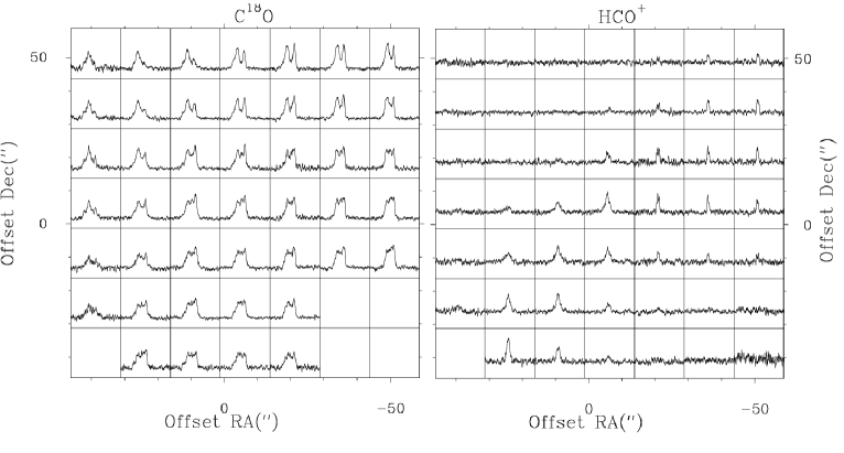
Figure 13: The spectra of C¹⁸O 3–2 and HCO⁺ 4–3 of the LFAM 26 field. The intensity scale is -1 to 6 K in $T_{\rm{MB}}$ for C¹⁸O and -1 to 3 K for HCO⁺. OphE-MM3 is located at $\Delta$RA = +5^′′ and $\Delta$Dec = -40^′′ in this field and has no associated HCO⁺ emission, except from the extended cloud.

Figure 14: Individual spectra at offset positions from LFAM 26 for HCO⁺ (0^′′,0^′′) and C¹⁸O (0,0), (-50,50), (10,50) and (25,-40). The three main components at 3.5, 4.4 and 5.0 km s^-1 are shown with solid lines. The component at 2.7 km s^-1 identified by Boogert et al. (2002) is shown with a dashed line and is generally weaker or absent. The main component of the HCO⁺ emission is located between the components at 4.2 and 4.9 km s^-1 and peaks at 4.6 km s^-1.

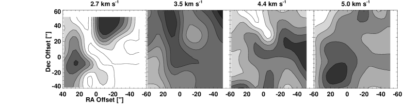
Figure 15: The spatial distribution of the integrated gaussians fitted to the C¹⁸O 3–2 spectra for each of the four layers seen in the field of LFAM 26.

Table 5: The number and properties of the (foreground) layers for the fields of LFAM 26, IRS 44 and WL 19 in the Ophiuchus ridge and IRS 37 and IRS 4, located near Oph-B cores, see Fig. 7.

Field	Position	Nr. comp	$V_{\rm{LSR}}$ (km s-1)	C18O $\int T_{\rm{MB}}dV$ (K km s-1	$\Delta V$ (km s-1)
LFAM 26	0,0	3	3.5, 4.4, 5.0	1.8, 0.9, 1.1	0.8,0.7,0.8
	-20,+35	4	2.7, 3.5, 4.4, 5.0	0.6, 1.5, 0.8, 1.1	0.9, 0.7, 0.7, 0.7
	+35, -22	3	3.5, 4.4, 5.0	1.3, 0.4, 0.5, 1.2, 0.7,0.5
IRS 44	0,0 a	3	2.6, 3.5, 4.5	0.5, 2.3, 2.3	1.9,1.1, 0.8
	+20,+20 (IRS 46)	2	3.5, 4.3	1.9, 1.3	0.6,0.5
	-50,20	2	3.3, 4.0	1.1,2.5	0.4, 1.1
IRS 48	0,0	3	2.8, 3.5, 4.1	0.6, 1.7, 2.6	0.6, 0.4, 0.5
	-36,+36	3	2.9, 3.5, 4.1	0.8, 2.1, 4.3	0.4, 0.4, 0.5
	+38, 6	3	2.8, 3.5, 4.1	0.4, 1.1, 3.5	0.3, 0.5, 0.5
WL 19	0,0	2	3.3, 4.6	2.7, 4.7	0.8,0.8
	-6, 36	2	3.4, 4.6	2.8, 5.6, 1.1,0.8
	-20,-38	2	3.2, 4.2	1.9, 3.0	0.7, 1.0
	-50, 50	4	2.6, 3.5, 4.3, 5.1	1.4, 3.3, 3.5, 3.2	0.5, 0.6, 0.7, 0.7
IRS 37	0,0	2	3.0, 4.4	2.3, 5.6	0.7, 1.1
	+23, +7 (WL3)	2	3.2, 4.4	2.7, 5.4	0.8, 1.0
	-36, 21	3	3.0, 3.6 , 4.2	2.4, 0.8, 2.8	0.9, 0.2,0.8

^aAn outflow is detected at 0,0 in HCO⁺ 4–3 which is probably the component seen at 2.6 km s^-1

In contrast with deeply embedded Class 0 YSOs, the environment around the embedded Class I YSOs has a large influence on the analysis of the generally weaker source data. Fig. 7 in Boogert et al. (2002) illustrates how complex the environment can become. Elias 29, an embedded YSO, is located in a dense ridge of material, but in front of that ridge, two foreground layers were identified using the emission from a dozen different molecules. Continuum emission and ice absorption originate in all these layers. For most of our sources, however, the situation appears to be less complex. Fig. 6 and 7 show that the HCO⁺ 4–3 profiles are mostly single peaked. However, C¹⁸O 3–2 often shows a more complex profile with multiple peaks.

LFAM 26, located at the top of the Ophiuchus ridge only a few arcmin north-east of Elias 29, is an especially complex case. Fig. 13 shows the spectral map in 17^′′ spatial bins for HCO⁺ 4–3 and C¹⁸O 3–2 maps. It is clearly seen that besides the integrated emission (Fig. 3), the line profiles of HCO⁺ and C¹⁸O both vary over the entire map. The HCO⁺ spectra show mostly single gaussians. At the position of LFAM 26, the HCO⁺ profile has a small outflow signature on the blue side of the spectrum. The C¹⁸O emission requires at least four distinct components (Fig. 14) at 2.7, 3.5, 4.4 and 5.0 km s^-1. The three components at 2.7, 3.5 and 5.0 km s^-1 are the same as found in Boogert et al. (2002) at the position of Elias 29. Most lines observed in Boogert et al. (2002) peak short-wards of 5.0 km s^-1 component, which could be indicative of the 4.4 km s^-1 component . However, the difference between these two components is very pronounced in the spectra in Fig. 13 and 14 at the position of LFAM 26 so that we treat them as separate. HCO⁺ is aligned with the 4.4 km s^-1 component.

Using the molecular excitation program RADEX (van der Tak et al. 2007), one can calculate the expected average contribution from cloud material to the HCO⁺ 4–3 emission. Using a HCO⁺ abundance of 10^-8 with respect to H₂, a density of 10⁴ cm^-3, a cloud temperature of 15 K, a width of 1 km s^-1 and a H₂ column density of 10²² cm^-2 ($A_{V}\approx$ 10), a contribution of $\sim$ 0.1 K km s^-1 is found. Only at higher column ($\sim$10²³ cm^-2) or volume densities ($\sim$1$\times$10⁵ cm^-3) are contributions found from the cloud on the order of 1 K km s^-1, comparable to the observed 4.4 km s^-1 emission at off-positions such as (-50,50). This is in agreement with the numbers given in Table 1 of Evans (1999). Thus, LFAM 26 is embedded in a high-density ridge.

Table 5 shows the results of gaussian fitting at other positions where multiple peaks in the C¹⁸O 3–2 profiles were found. In the WL 19 field, south of the Elias 29 position, the same four components are again detected, although the 5.0 km s^-1 layer is only seen north of WL 19. In the IRS 44 field along the same ridge to the south-west, the three layers at 2.6, 3.5 and 4.5 km s^-1 are found.

Three layers are found in the Oph-B2 core, which contains the IRS 48 and IRS 37 sources. The first layer is at 2.8 km s^-1, the second at 3.5 km s^-1 and the third at 4.2 km s^-1. Outside these two regions, spectra of C¹⁸O can be fitted with a single gaussian, almost always at $\sim$ 3.6 km s^-1. The spatial variation in this layer seems to be minor compared with the other components and it is thus the most likely candidate for the foreground component with an extinction of $A_{\rm{v}}\sim$5.5 mag, as suggested by Dickman & Herbst (1990). IRS 63, located far from the L 1688 core is at 2.8 km s^-1, the same velocity as one of the layers in both Oph-B2 and Ophiuchus ridge region.

5.3 Gas column density

The total column density, $N_{\rm{H_{2}}}$, toward each source was calculated from the integrated intensity of the C¹⁸O 3–2 line,$\int T_{MB}$ dV, using the following formula :

$$N({\rm H_{2}})=X\times 0.75\times 10^{14}\frac{e\>^{(16.6/T)}\int T_{MB}dV}{1-e\>^{(-33.2/T)}}$$ (3)

with $X$, the abundance of H₂ with respect to C¹⁸O, assumed to be 5.6$\times 10^{6}$ (Wilson & Rood 1994) and $T$, the temperature of the cloud material, assumed to be 30 K. The temperature is chosen to be higher than that of the surrounding cloud material, $\sim$15 K, and reflects the warmer gas associated with the YSO where CO is not frozen out. This formula assumes the molecular excitation to be in LTE and isothermal. The C¹⁸O 3–2 line is assumed to be completely optically thin. The resulting column densities can be found in Table 4, column 3. They range from 3.7$\times$10²² cm^-2 for IRS 63 and the Oph F core to 31.6 $\times$10²² cm^-2 in the Oph A core. These correspond to visual extinctions $A_{V}$ of 40-400 mag , assuming $N_{\rm H}/$$A_{V}$ =1.8$\times 10^{21}$ cm^-2 mag^-1 (Rachford et al. 2002) and $N_{\rm H}\approx 2N($H₂) (all hydrogen in molecular form). This range of column densities is similar to that found by Motte et al. (1998) and Stanke et al. (2006) using 1.3 mm continuum imaging, as well as the column densities found from the 850 $\mu$m dust, see $\S$5.4.

Figure 16: Left : the gas column density (in 10²² cm^-2) derived from C¹⁸O 3–2 vs. the envelope mass (in 10^-2 M_⊙), derived from the SCUBA maps; middle : the column density vs. the integrated intensity of HCO⁺ 4–3 in K km s^-1 and right : the integrated intensity of HCO⁺ 4–3 vs. the envelope mass . In all figures, sources with a centrally condensed HCO⁺ emission are shown with stars, sources with an upper limit on HCO⁺ 4–3 with triangles, and sources with HCO⁺ emission not peaking on the source with diamonds.

5.4 Dust

Table 4 includes the properties that can be derived from the continuum emission. The dust column density was calculated with the following equation.

$$N({\rm H_{2}})=\frac{S_{850}}{\Omega\;\mu\;m_{H}\;\kappa_{850}\;B_{850}(T_{d})}$$ (4)

where $S_{850}$ is the flux in the central beam, $\Omega$ is the main beam solid angle of 15^′′, $\mu=2.33$ the mean molecular weight, $m_{\rm H}$ the mass of atomic hydrogen, $\kappa_{850}$ the dust opacity per gram of gas and dust at 850 $\mu$m and $B_{850}(T)$ the Planck function at 850 $\mu$m for a temperature $T$, assumed to be 30 K. A $\kappa_{850}$ = 0.01 cm² gr^-1 is adopted from Ossenkopf & Henning (1994) for dust with thin ice mantles (Table 1, column 4).

Two assumptions affect the comparison between the column densities derived from C¹⁸O and those from dust continuum. C¹⁸O can be frozen out onto the dust grains below $\sim$30 K at sufficiently high densities, so that C¹⁸O column densities are expected to be lower than those obtained from dust data. Second, all dust emission is assumed to originate in envelope or cloud material, whereas for several sources the disk contributes significantly to the continuum. These combined effects likely eplain the lack of correlation seen in Fig.16 (left)

If one assumes that all emission detected at 850 $\mu$m is associated with an isothermal envelope, a source mass can be determined following Equation 4 from Shirley et al. (2000):

$$\begin{split}M_{D}\;=\;\frac{S_{850}\;D^{2}}{B_{\nu}(T_{d})\;\kappa_{\nu}}=3.69\;\times\;10^{-6}\;M_{\odot}\\ \times\;S_{850}(\rm{Jy})\;D^{2}(\rm{pc})\;\times\;(e^{16.9/T_{d}}\;-\;1)\end{split}$$ (5)

Since the 3$\sigma$ sensitivity of the COMPLETE map is 80 mJy within a 15^′′ beam, the lower limit to the detectable mass is 0.04 M_⊙. Such a low mass implies either a source that has nearly shed its envelope and is close to the pre-main sequence phase or an intrinsically very low luminosity object (Dunham et al. 2008).

Fig. 16 shows the relation between the different column densities, envelope masses and the presence of dense gas as traced by HCO⁺. These figures clearly show that at higher envelope masses, the amount of dense gas and the total envelope mass correlate. The third figure illustrates that nearly all sources with centrally concentrated HCO⁺ emission have larger envelope masses. Above an envelope mass of 0.1 M_⊙, only a single source that is classified as confused in $\S$ 6 (indicated with diamonds) is seen with HCO⁺ $>$ 2 K km/s. This is CRBR 2422.8-3423, which is located in the line of sight with the envelope of IRS 43. The high mass found for CRBR 2422.8-3423 can be fully attributed to this envelope.

5.5 Effect of reddening on $\alpha_{\rm IR}$

Foreground material reddens the YSO and steepens the spectral slope $\alpha_{\rm{2-24\mu m}}$. An estimate can be made of the foreground column density based on our C¹⁸O maps, by assuming that the average column or $A_{V}$ at 45^′′ offset from the source position in all directions originates entirely from this cloud. Although it is not known a priori whether this material is foreground, back-ground, or a different YSO, we assume here that it is all foreground (see also §5.2) which provides an upper limit to the reddening. Note that the column densities at these positions were calculated with a temperature of 15 K, a temperature associated with the surrounding cloud, instead of 30 K, a temperature associated with protostellar envelopes. For typical dust opacities and the $A_{V}$=5.5 mag layer as suggested by Dickman & Herbst (1990), $\alpha_{\rm 2-24\mu m}$ is only increased by 0.18 (see also Crapsi et al. (2008)). However, for higher $A_{V}$ of $\sim$ 40 mag, as commonly found in the Ophiuchus ridge, this correction can be as high as 1.1, enough to change the classification of a Class II T Tauri star with disk to an embedded Class I source. Table 4 includes the (maximum) change in $\alpha_{\rm 2-24\mu m}$ due to foreground reddening for each source derived by this method. Chapman et al. (2008) probe the $A_{K}$ in the northern part of Ophiuchus, including the northern part of the Oph-A area, where $A_{V}$ values of 40 mag. and higher are found. In the Oph-A, Oph-B2 and Ridge regions, $A_{V}$ of this magnitude were found from C¹⁸O column densities, reinforcing the conclusion that a strong extinction affects these regions on scales of only a few arcminutes, a resolution often not reached by extinction studies (Cambrésy 1999). Although these numbers have large uncertainties, they do illustrate the point that this potential extreme foreground reddening can lead to incorrect classifications for a significant number of sources in Ophiuchus.

An alternative is to use the velocity resolved C¹⁸O spectrum at the source position but subtract the layer that includes the source. For example, LFAM 26 ($\Delta\alpha_{\rm{IR}}$=4.4), resides in a dense ridge (see $\S$ 5.2). Subtracting the gaussian profile of this layer at $\sim$4.4 km s^-1 gives an integrated intensity of 2.9 K km s^-1, which corresponds to a column density of 10.7$\times 10^{22}$ cm^-2, an $A_{V}$ of $\sim$60 mag and $\Delta\alpha_{\rm{IR}}$ = 3.2. If one assumes that the layers are arranged in distance in order of increasing $V_{\rm{LSR}}$, only the front layer at 3.5 km s^-1 will redden and a column density of 6.6$\times 10^{22}$ cm^-2, an $A_{V}$ of $\sim$40 and $\Delta\alpha_{\rm{IR}}$=1.9 are found. Thus, $\Delta\alpha_{\rm{IR}}$ is likely to be in between the maximum value listed in Table 4 and $\Delta\alpha_{\rm{IR}}/2$, although exceptional cases, such as OphE-MM3, an edge-on disk in front of the cloud, do exist.

5.6 SEDs: $L_{\rm Bol}$ and $T_{\rm Bol}$

The IR and submillimeter fluxes have also been used to calculate the bolometric luminosity, $L_{\rm{bol}}$, and temperature, $T_{\rm{bol}}$, of each source. These numbers were calculated using the prismodial or the midpoint methods, with the inclusion of the 2MASS, IRAC, MIPS-24, MIPS-70, SHARC-II, SCUBA and 1.3 mm fluxes. Only fluxes with a $S/N>$ 5 were included. For a more thorough discussion on the useage of these two methods, see Dunham et al. (in prep.) and Enoch et al. (2008).

Table 6 compares the values found for $T_{\rm{bol}}$ and $L_{\rm{bol}}$ in our work with those of Evans et al. (2009) for several sources. The differences stem from the fact that Evans et al. (2009) use CSO-Bolocam 1.1 millimeter data in a 30^′′ beam, together with 2MASS, IRAC, and MIPS (24, 70 and 160 $\mu$m) fluxes. No SHARC-II or SCUBA fluxes were included, nor were sources with no detection at 1.1 mm. As can be seen from the results for Elias 29 and GSS 30 IRS1, the inclusion of Bolocam and MIPS-160 produces a higher $L_{\rm{bol}}$ of up to a factor of 6. In addition, $T_{\rm{bol}}$ is consistently lower for the brighter sources. This can be largely attributed to the contributions from the surrounding cloud, which add significantly to the MIPS-160 and Bolocam fluxes. Although cloud emission is present in the IRAM-30m 1.3 mm and SCUBA-850 $\mu$m observations used in our studies, the higher resolution of 15^′′ limits such contributions. The exclusion of MIPS-160 in our work causes the $L_{\rm{bol}}$ to be underestimated and the $T_{\rm{bol}}$ to be overestimated, due to the lack of a point at far-IR wavelengths near the peak of the SED. Isolated, unresolved sources such as IRS 42 show little to no differences between the two studies, confirming the influence of the environment. Future high resolution ($<$10^′′) observations with the PACS instrument on Herschel covering the 60 to 600 $\mu$m window will be able to fully constrain the far-IR emission and SED.

Table 6: Comparison between $L_{\rm{bol}}$ and $T_{\rm{bol}}$ as calculated in Evans et al. (2009) (indicated with Evans) and this work (indicated with van K.).

Source	$L_{\rm{bol}}$	$L_{\rm{bol}}$	$T_{\rm{bol}}$	$T_{\rm{bol}}$
	Evans	van K.	Evans	van K.
	($L_{\rm{\odot}}$)	($L_{\rm{\odot}}$)	(K)	(K)
GSS 30	8.7	3.3	150	123
CRBR 2339.1	$<$0.065	0.055	$<$370	426
WL 2	0.12	0.09	428	573
LFAM 26	0.15	0.044	110	238
WL 17	0.6	0.67	310	323
Elias 29	17.9	2.5	257	424
IRS 42	1.2	1.4	600	540
CRBR 2422.8	0.19	0.44	$<$300	157
IRS 43	3.8	1.0	160	134
IRS 44	15	1.1	110	140

5.7 Ice and silicate absorption

In the online appendix, the IRS spectra for 28 of the sources in our sample are plotted. 17 sources show ice absorption bands at 15.2 $\mu$m due to CO₂ ice (see Table 7), and 11 do not (WL 3, LFAM 26, VSSG 1, CRBR 2317.3, CRBR 2315.8, IRS 48, CRBR 2339.1, SR 21, Haro 1-4, IRS 46 and SR 9). A few of the known edge-on disks, such as CRBR 2422.8-3423.2, show ice absorptions.

Crapsi et al. (2008) modelled the spectral features at 3 $\mu$m (H₂O ice), 10 $\mu$m (silicate) and 15.2 $\mu$m (CO₂ ice) for a large grid of models, including embedded sources and T Tauri disks, both seen at a wide variety of angles. The ice absorptions at 3 and 15.2 $\mu$m were found to be more prevalent for embedded sources. However, edge-on disks can also show such absorptions in almost equal strength. The relation of the 3 $\mu$m ice absorptions with the envelope mass of both embedded and disk sources is given in Fig. 4 of Crapsi et al. (2008) and a similar relation was found for the 15.2 $\mu$m band. Cold foreground clouds can also contribute significantly.

Using the determination of the column densities from the C¹⁸O and SCUBA maps in $\S$ 5.3 and 5.4, Eq. 3 and 4, the ice absorption can be compared to the amount of reddening as indicated by $\Delta\alpha_{\rm{IR}}$. Although ice absorptions are more commonly found in sources with a higher reddening, it is concluded that the YSOs must be characterized on a source by source basis to locate the origin of the ices. The disk source CRBR 2422.8 has deep ice absorptions (Pontoppidan et al. 2005), most likely originating the large column of foreground material ($\Delta\alpha=0.9$). However, LFAM 26, which has an even higher reddening ($\Delta\alpha=1.7$), shows no sign of ice absorption. Of course, it is possible LFAM 26 is located in front of the cloud and as such the presence or absence of ice absorption could serve as a useful diagnostic of the geometry of the YSO-cloud system. The silicate feature around 10 $\mu$m is detected for fewer sources than the 15.2 CO₂ ice absorption. Although LFAM 26, WL17, Elias 29, IRS 42, WL 3, IRS 54, CRBR 2315.8-1700, CRBR 2339.1-2032 and CRBR 2422.8-3423 all have silicate absorption, many other sources were not observed at the wavelengths of the silicate feature.

6 Classification

Table 7: The classification of the source sample with the recipe outlined in the text.

Source	Codea	Stage
Embedded sources
GSS 30	SHC8 EH8 PH8I	1
LFAM 1	SH8 NC EH8 PH O8	1
VLA 1623	SHC8 EH8 PH8	0
WL 12	SHC8 EHC8 PHC8I	1
LFAM 26	SHC8 EHC8 PH8 OC	1
WL 17	SH8 NC PH8I	1(T)
Elias 29	SHC8 EH8 PH8I	1
IRS 37	SHC W8 EHC8 PHC8I	1
WL 3	SHC W8 EHC8 PH	1
WL 6	SHC N8I	1(T)
IRS 43	SHC8 EH8 PH8I	1
IRS 44	SHC8 EHC8 PHC8	1
Elias 32	SHC8 EH8 PH8I	1
Elias 33	SHC8 EH8 P8I	1
IRS 54	SHC W8 EHC8 PHC8I	1(T)
IRAS 16285-2355	SH8 WC EHC8 PHC8	1
IRS 63	SH8 WC EHC8 PHC8I	1(T)
Confused Sources
CRBR 2324.1-1619	SHC8 EHC8 OHC8	C
GY51	S8 NHC E8 O8	C
WL19	SC8 NH EHC8 OHC8I	C
IRS 42	SHC8 EH8 OH8I	C
GY 256	SHC N8	C
Disks
SSTc2d J162527.6-243648	NHC8	2
GSS 26	S8 NHC P8	2
CRBR 2315.8-1700	SH8 NC EH P8 OH	2
CRBR 2317.3-1925	SH W8 NC	2
VSSG 1	W8 NHC P8	2
CRBR 2339.1-2032	SH W8 NC P8	2
WL 2	WH8 NC EH8 OH8	2
GY 224	W8 NHC P8I	2
WL 20S	SC8 NH P8I	2
IRS 48	WC8 NH EC P8	2
GY 312	NHC8	2
IRS 51	SH8 WC EHC8 P8 OHCI	2
SSTc2d J162741.6-244645	W8 NHC	2
SSTc2d J162748.2-244225	NHC8	2
SSTc2d J162857.9-244055	S8 NHC	2
Haro 1-4	NHC8	2
DoAR 25	S8 NHC P8	2
OphE MM3	SHC W8 EHC8 OH8	2
SR 21	W8 NHC P8	2
CRBR 2422.8-3423	SH8 NC E8 O8I	2
IRS 46	S8 WC NH EHC8 OHC8	2
SR 9	NHC8	2
2Mass 16282	W8 NHC	2

^aThe coding in column 2 is as follows:
S, W and N determine if a line or continuum is Strong, Weak or Not detected/observed.
E, P and O determine if a source is Extended, Peaking or Offset peaking.
The subscripts H, C and 8 refer to the HCO⁺, C¹⁸O and 850 $\mu$m.
I is detected CO₂ ice absorption. Column 3 lists the classification. 1 is a Stage 1 embedded YSO, 2 is a disk and C is Confused.

6.1 Physical classification

A new classification based on physical parameters has gradually been introduced (Whitney et al. 2003b; a, Robitaille et al. 2006) but is not yet as commonly in use as the traditional Class system. This new classification identifies the evolutionary stage using the physical characteristics as opposed to the observed characteristics. The different evolutionary stages are determined from the ratios between $M_{\rm{disk}}$, $M_{\rm{envelope}}$ and $M_{\rm{star}}$. The total circumstellar mass, $M_{\rm{circum}}$, is defined as $M_{\rm{disk}}$+$M_{\rm{envelope}}$. The evolutionary stages of this classification are:

• Stage 0, deeply embedded sources with $M_{\rm{disk}}$/$M_{\rm{envelope}}$ $<<$ 1 and $M_{\rm{circum}}$/$M_{\rm{star}}\sim$ 1

• Stage 1, embedded sources with 0.1 $<$ $M_{\rm{disk}}$/$M_{\rm{envelope}}$ $<$ 2 and $M_{\rm{circum}}<$ $M_{\rm{star}}$

• Stage 2, classical T Tauri stars with gas-rich disks ($M_{\rm{envelope}}$ = 0 and $M_{\rm{disk}}$/$M_{\rm{star}}$ $<<$ 1 )

• Stage 3, Pre-main sequence stars with tenuous disks.

Stage 0 sources are equivalent to Class 0 sources and can be identified by their submm characteristics as originally put forward by André et al. (1993). Stage 2 and Stage 3 sources, corresponding to the classical T Tauri stars with disks and pre-main sequence stars with (gas-poor) tenuous disks, are identified using the IR excess combined with optical/near-IR spectroscopic properties. The amount of IR excess and the wavelength where this excess starts are often used to distinguish Stage 2 and 3 sources.

The Stage 1 sources are most problematic to uniquely identify based on observational characteristics. Both Whitney et al. (2003a) and Crapsi et al. (2008) show that the traditional identification methods of using the IR spectral slope $\alpha_{\rm{IR}}$ and $T_{\rm{bol}}$ are insufficient to distinguish the edge-on disks from embedded sources, as well as missing evolved, face-on embedded YSOs that are (mis)classified as Class II. One of the main parameters to unambiguously identify Stage 1 sources is the $M_{\rm{disk}}$/$M_{\rm{envelope}}$ ratio as determined from millimeter continuum observations in a large and small ($\sim 2^{\prime\prime}$) beam (Crapsi et al. 2008). However, the interferometric observations needed to unambiguously constrain the disk masses are still time-consuming for large samples of sources.

6.2 Identifying embedded stage 1 sources with molecular emission

To uniquely identify embedded sources and distinguish them from edge-on disks, prestellar cores and possible background AGB stars and galaxies without having to resort to interferometers, we propose to use the single-dish molecular emission. Embedded sources will be bright and centrally peaked in HCO⁺ 4–3 and C¹⁸O 3–2. The HCO⁺ line maps will detect all but the most tenuous envelopes. The concentration parameter shows that HCO⁺ 4–3 is much more accurate in identifying protostellar envelopes than continuum dust emission. The HCO⁺ maps also spatially resolve larger envelopes (e.g., the VLA 1623 and GSS 30 envelopes). The nearby environment, including foreground layers, is in turn characterized by the C¹⁸O 3–2 (see $\S$ 4 and 5).

To distinguish embedded sources from isolated edge-on disks, a good limit on the HCO⁺ 4–3 emission is $T_{\rm{MB}}>$ 0.4 K. Thi et al. (2004) observed four well-studied gas-rich disk sources in a large range of molecular transitions, including HCO⁺ 4–3, and found $T_{\rm{MB}}\sim$ 0.1 K, four times below our adopted limit. Although disks around embedded sources could be somewhat larger and more massive, it is assumed that the contribution from even the largest embedded disks does not exceed our adopted limit. This value is naturally small because of the severe dilution of emission originating in a disk within the 15 $"$ JCMT beam. For example, a 20 K optically thick line from a 2^′′ disk would be diluted to 0.35 K. Indeed, for two embedded sources for which interferometric HCO⁺ data exist (IRS 63 and Elias 29, Lommen et al. (2008)), the HCO⁺ contribution of the disk does not exceed this limit (see §6.3).

The following definitions were therefore used to classify the sample:

• Stage 1

  • Extended HCO⁺ emission, peaking on source, with $C_{\rm HCO^{+}}>$ 0.7 and $\int T_{\rm{MB}}$dV $>$ 0.4 K km s^-1 and/or

  • an HCO⁺ profile that is not extended, but $\int T_{\rm{MB}}$dV $>$ 0.4 K km s^-1, with SCUBA both extended and $C_{850}>$ 0.7.

  • Ice absorptions are usually prominent.

• Stage 2

  • Absence of HCO⁺, SCUBA and C¹⁸O down to the rms limits at the IR position or

  • no variation of HCO⁺, SCUBA and C¹⁸O on scales of 30^′′ ($C<$ 0.4) or

  • no C¹⁸O 3–2 or SCUBA is seen at scales larger than the central beam of 15^′′ with HCO⁺ 4–3 not extended and $<$ 0.4 K km s^-1 or

  • $\alpha_{\rm{IR}}<$ -0.5.

• Confused

  • HCO⁺, SCUBA or C¹⁸O peaking more than 20^′′ away from the IR position
    

In the rare case that an embedded source is viewed face-on (into the outflow cone, see Whitney et al. (2003b)), the above restrictions will identify such a source as stage 1, having $\alpha_{\rm{IR}}<-0.3$, but with extended HCO⁺ emission, peaking on source ($\int T_{\rm{MB}}$dV $>$ 0.4 K km s^-1).

Table 7 shows the results for this classification. In Appendix C the sources and their classifications are discussed on a source by source basis. Sixteen Class I sources were identified as embedded Stage 1 sources with envelopes varying in mass and size. The sources GSS 30 IRS 1 and LFAM 1 appear to be embedded within an approximately spherical envelope encompassing both sources. The sources IRS 37 and WL 3 are embedded in a highly non-spherical envelope covering both sources. In addition to these 16 sources, VLA 1623 is classified as embedded, but considered a Stage 0 source due to its high sub-mm flux relative to the total luminosity. From comparison with Jørgensen et al. (2008) (see $\S$ 6.5), we can conclude that all embedded sources were found down to a mass limit (envelope+disk) of 0.04 M_⊙. Deep searches for even lower luminosity sources have found only two likely candidate sources within our field (Dunham et al. 2008). Deep (interferometric) sub-mm observations are needed to identify if such sources are truly embedded.

Five sources were found to be confused (C in Table 7). The exact nature of these sources (obscured, disk or other) cannot be determined without interferometric observations. However, molecular emission rules out a protostellar envelope. Observations of C¹⁸O show that cloud material is located in the line of sight towards these sources. They will be further discussed in $\S$6.4.

Twenty-three sources were found to be Stage 2 sources (2 in in Table 7). Of this sample, sources with $\alpha_{\rm{IR}}>0$ and with no correction from extinction (see Table 4) are likely to be edge-on or close to edge-on disks. Sources that do have a potential correction to $\alpha_{\rm{IR}}$, such as CRBR 2422.8 or IRS 48, do not have to be edge-on. All sources that were initially known to be disk sources are identified as Stage 2 sources using this method. If one considers that disk sources with $\alpha_{IR}$ $>$-0.3, when corrected for the maximum $\Delta\alpha_{\rm{IR}}$), are edge-on, only 7 out of 23 Stage 2 sources of our sample are expected to be edge-on. The total amount of Class II sources found in Ophiuchus by c2d is 176, and although this includes L 1689, the bulk of these disks exist close to or are part of the L 1688 region (Evans et al. 2009). Thus, our number of edge-on disks appears to be only a small fraction of the total disk sample.

No face-on embedded sources were found that have $\alpha_{\rm{IR}}<-0.3$, but do show a HCO⁺ spectrum that is both peaking on source and stronger than 0.4 K km s^-1. This very low fraction is not surprising, since such sources have strong restrictions on the line of sight.

Using the results from Spitzer (Evans et al. (2007), Jørgensen et al. (2006), Evans et al. (2009), Allen et al. in prep) a comparison can be made between the classification using $\alpha_{\rm{IR}}$ and the new method. It is found that $\sim$50$\%$ (11 out of 22) of the sources classified as Class I are Stage 2 disks and not embedded. Note that this includes the known disks OphE MM3 and CRBR 2422.8. However, of the Flat spectrum sources, $\sim$50$\%$ (6 out of 13) appear to be embedded, while the other half is either confused or classified as a Stage 2 disk. In the end, the sample of embedded sources found by c2d changes from 22 out of 45 to 17 out of 45.

Table 8: Comparison between the classification of YSOs using $\alpha_{\rm{IR}}$ by Evans et al. (2009) and our method using molecular emission.

	Class I	Flat Spectrum	Class II	Total
Stage 1	11	6	0	17
Confuseda	1	3	1	5
Stage 2	10	4	9	23
Total	22	13	10	45

^aNote that although it is possible for Flat Spectrum sources to be embedded, confused sources are ruled out to be embedded.

6.3 Late stage 1 sources

Of the sixteen embedded Stage 1 sources, four sources (WL 6, WL 17, IRS 54 and IRS 63) were found to have only marginal envelopes left, with C¹⁸O and 850 $\mu$m emission suggesting that at most a few $\times 0.01M_{\odot}$ remains in the envelope. Lommen et al. (2008) observed IRS 63 using the Sub-Millimeter Array (SMA) and found that 50 % of the continuum emission originates within a disk no bigger than 200 AU in size with a mass of 0.055 $M_{\rm{\odot}}$ and the remainder in a remnant envelope with a mass of 0.058 $M_{\rm{\odot}}$. HCO⁺ 3–2 was also detected with the SMA, originating mostly in the disk. When convolved with the JCMT beam, the observed brightness is 0.28 K km s^-1. The HCO⁺ 4–3 single-dish intensity as observed with HARP-B is 0.75 K km s^-1, 3 times as bright. For typical disk excitation conditions, HCO⁺ 4–3 is expected to be equal or weaker compared to the 3–2. It can thus be concluded from the much higher observed intensity in the 4–3 line, that at least half of the 4–3 emission within the JCMT beam likely originates in the protostellar envelope and would not be seen by the SMA.

In all four sources, little to no extended C¹⁸O is seen. The distributions and strengths in the HCO⁺ and C¹⁸O lines of the other three sources are similar to that of IRS 63, but the SCUBA image of IRS 63 is a factor of 4 brighter. For IRS 54, the envelope is spatially resolved in HCO⁺, C¹⁸O and SCUBA.

Although rare, it is concluded that these sources are Stage 1 sources in transition to a Stage 2 source (marked with 1(T) in Table 7). They have accreted or dispersed almost their entire envelope. Continuum emission in the sub-mm is likely to contain a large contribution from the protostellar disk.

6.4 Confused sources

For the five confused sources, CRBR 2324.1-1619, GY 51, WL 19, IRS 42 and GY 256, the exact nature cannot be determined using HCO⁺, except that such sources are ruled out as embedded YSOs. None of them have the characteristic peak of HCO⁺ that most Stage 1 embedded YSOs have. However, at least two out of the three tracers, HCO⁺, C¹⁸O and SCUBA, are detected so a few possibilities remain. The first is an (edge-on) disk, in front of cloud material. This would be similar to the case of OphE-MM3, which was confirmed to be an edge-on disk in front of a dense core (Brandner et al. 2000). Without the near-IR imaging, OphE-MM3 would have been classified as confused. A second possibility is that they are background sources. The most likely options are then a T Tauri star with disk behind the cloud (possibly edge-on), or an AGB star. Background main sequence stars are identified within the c2d delivery document (Evans et al. 2007) and are thus highly unlikely to be included in our sample. Chances of background AGB stars or galaxies being aligned with the cloud are small, but according to Jørgensen et al. (2008), a single background source can be expected. A final possibility is that the sources are very late Stage 1 embedded YSOs, very close to the Stage 2 phase. An upper limit of only 0.02 M_⊙ is found for their envelope mass.

6.5 Comparison to other methods

Fig. 17 shows the effectiveness of the classification of sources using the method above, as compared to methods using $\alpha_{\rm{IR}}$ and $T_{\rm{bol}}$. A key parameter is the strength of the HCO⁺ integrated intensity. The following limits were adopted between embedded and disk sources: $\alpha_{\rm{IR}}>0$, $T_{\rm{bol}}<650$ K and HCO${}^{+}>0.4$ K km s^-1.

Figure 17: Classification of sources using the spectral slope (upper left), bolometric temperature (upper right), HCO⁺ intensity (lower left) and HCO⁺ intensity combined with the bolometric temperature (lower right). In the upper two plots, embedded sources are shown with a diamond, disks are shown with a star, and confused sources with a triangle. In the lower two plots, diamonds are again embedded sources, stars represent sources with an upper limit on the HCO⁺ and triangles are sources with no HCO⁺ peak associated with the source. Note that the confused sources and disk sources are both represented with triangles and stars. The traditional limits used for classification, $\alpha_{\rm{IR}}>$0 and $T_{\rm{bol}}<650$ K as well as our criterion, HCO${}^{+}>0.4$ K km s^-1, are shown with dashed lines.

The advantages of the method using molecular emission are immediately apparent. Although the classical methods of using $T_{\rm{bol}}$ and $\alpha_{\rm{IR}}$ are able to identify embedded sources, both methods also incorrectly identify a number of Stage 2 disks as embedded, especially for $L_{\rm{bol}}<1$ L_⊙. These are the edge-on disks. If one uses the limits of the integrated intensity for HCO⁺, isolated disk sources are easily identified. With the additional restriction of having a peak within the HCO⁺ map, confused sources or sources in front of the cloud can be readily identified.

The use of ice absorption, as studied by Crapsi et al. (2008), is limited by similar constraints. Most embedded sources, with the exception of LFAM 26 and WL 3, show CO₂ ice absorption at 15.2 $\mu$m. However, 4 disk sources IRS 51, WL 19, WL 20S and CRBR 2422.8-3423 also show strong ice absorptions. These ice absorptions are caused both by the foreground layers as discussed in $\S$5.2 as well as the material in the disk itself, if viewed edge-on (as is the case for CRBR 2422.8). Thus, the presence of ice absorption cannot be used to unambiguously identify embedded sources from other sources. Even if the origin of the ice absorption can be attributed to a protostellar envelope, its strength does not seem to be an indication of evolution, e.g. IRS 63, a small envelope, has a deeper ice absorption than the large envelope of GSS 30.

Jørgensen et al. (2008) published a list of ‘candidate’ embedded YSOs based on two criteria. First the colors of sources using the IRAC and MIPS results ($[3.6]-[4.5]$ and $[8]-[24]$). Second, the proximity of MIPS sources to SCUBA cores. For these cores, the concentration is an important parameter. Although most candidate embedded objects are identified by both criteria, several sources are included in their list based on only a single one. Comparison between their list (Table 1 in Jørgensen et al. (2008) limited to L 1688, further referenced as JJ1) and the list in this paper yields the following results:

• Four embedded YSOs with SCUBA fluxes below the cut-off adopted by JJ1 ($<$ 0.15 Jy beam^-1, the very low envelope masses) are absent from the JJ1 list. Two of these sources (WL6 and IRS 54) are classified by us as late Stage 1 sources with little to no envelope left. The other two embedded YSOs not included in JJ1 are IRS 37 and WL 3.

• Four sources are included in the JJ1 list that have been classified as Stage 2 disks by our method. These are GSS 26, CRBR 2315.8, CRBR 2339.1-2032 and IRS 51. All four sources have associated SCUBA cores and MIPS detections. See the appendix for the classification reasoning of each of these sources.

7 Conclusions

A sample of young stellar objects in L 1688 was analyzed using gas mapping obtained with the new HARP-B heterodyne array receiver in the HCO⁺ 4–3 and C¹⁸O 3–2 lines. Complementary dust maps were obtained from the COMPLETE project, as observed by JCMT-SCUBA, and with SHARC-II on the CSO. The original sample consisted of 45 sources, mostly classified as embedded YSOs or flat-spectrum sources using their spectral slope $\alpha_{\rm{IR}}$ in previous work. Of this sample a few sources were recently discovered to be edge-on disks. As a control sample, 4 known disk sources in L 1688 were included. The observations were supplemented by single-pixel observations from APEX, Spitzer-IRS spectroscopy and continuum photometry ranging from 1 $\mu$m to 1.3 mm, using a variety of space-based and ground-based observatories.

The main conclusions are:

• The concentration of the dense gas, as traced by the HCO⁺ 4–3 line mapping, provides an excellent tool to characterize the dense gas in the inner regions of protostellar envelopes. Material in the cold outer envelopes, (edge-on) disks, prestellar cores or cloud material does not emit strongly in HCO⁺ 4–3.

• Most envelopes in L 1688 have low masses, ranging from 0.05 to 0.5 M_⊙. The main accretion phase onto the star has already taken place. The only exception is the Stage 0 source VLA 1623 which contains nearly 1 M_⊙.

• A new classification tool based on molecular emission to uniquely identify embedded sources is proposed. Of the total sample, 17 sources were found to be embedded, 5 sources were confused and 23 sources were identified as (edge-on) disks. Due to the foreground layers found through the C¹⁸O, it is concluded that a significant fraction of the sources previously classified as Class I or Flat Spectrum are disks and have been strongly reddened. Combined with the analysis in Jørgensen et al. (2008) all embedded sources in L 1688 were included and characterized down to a mass limit of 0.04 M_⊙ (envelope+disk).

• Four embedded YSOs are found that are in transition from the Stage 1 embedded phase to the Stage 2 T Tauri phase. These sources, IRS 63, IRS 54, WL 6 and WL 17, have little envelope left ($M_{\rm{env}}\sim 0.05M_{\rm{\odot}}$).

• Five sources are so confused by cloud material that identifying them as T Tauri disks or background sources is not possible with our data. The (lack of) variation and concentration of the molecular emission rules them out as embedded YSOs, however.

• All sources previously identified as disks using traditional methods such as $T_{\rm{bol}}$ and $\alpha_{\rm{IR}}$ are indeed recovered as disks as are all edge-on disk sources, identified by near-IR mapping (e.g. IRS 46, CRBR 2422.8-3423 and OphE-MM3).

• Spectral line mapping of C¹⁸O reveals that foreground layers are predominantly present in the Ophiuchus ridge and the Oph-B core. Outside these regions, foreground layers are absent. These foreground layers are responsible for heavy reddening with typical $A_{V}>20$, confusing classification schemes based on IR colors.

The YSOs in the Ophiuchus clouds show a wide variety of characteristics, ranging from the rare Stage 0 deeply embedded source VLA 1623 and Stage 1 embedded YSOs such as Elias 29, IRS 43 and WL 12 to the embedded YSOs with wimpy envelopes in transition to the T Tauri stage like IRS 63. The results above imply that the molecular emission maps uniquely characterize the envelopes associated with embedded YSOs, while simultaneously identifying disks erroneously classified as embedded YSOs. Such characterization is needed before statistical studies can be used to estimate time scales and star formation efficiencies within L 1688.

One characteristic that has yet to be determined is the ratio of the disk to envelope mass. Interferometric studies with advanced facilities such as the SMA, CARMA or the PdB interferometer will allow the disks to be characterized and, through comparison with continuum single dish studies, the envelope (e.g. Jørgensen et al. 2005, Lommen et al. 2008). Such detailed information will be necessary as a starting point for the interpretation of future observations with Herschel and ALMA of the embedded YSOs in Ophiuchus and other clouds. A central role is envisioned for molecular line data.

Table 9: Source fluxes including IRAC 1-4, MIPS 1-2, SHARC-II, SCUBA and 1.3 mm data.

Source	3.6$\mu$me	4.5$\mu$me	5.8$\mu$me	8.0$\mu$me	24$\mu$me	70$\mu$m	350$\mu$m	450$\mu$m	850$\mu$m	850$\mu$m	1300$\mu$m
	IRAC I	IRAC II	IRACIII	IRAC IV	MIPS I	MIPS II	SHARC	SCUBA	SCUBA	SCUBA
						$\sim$10′′	9-25′′b	10 ′′b	15′′	25′′	15′′
	mJy	mJy	mJy	mJy	mJy	mJy	mJy	mJy	mJy	mJy	mJy
C2D-162527.6	1.15e1	1.77e1	3.00e1	6.03e1	8.51e1	-	-	-	$<$3e1	$<$3e1
GSS 26	2.86e2K	3.86e2K	5.09e2	6.17e2	7.98e2	-		6.5e2	3.0e2b	1.6e3	1.e2
CRBR 2315.8-1700	4.53e1	8.77e1	1.61e2	2.37e2	5.16e2	-	-		2.1e2	7.5e2	8.5e1)
CRBR 2317.3-1925	1.05e1	1.15e1	1.39e1	2.05e1	1.46e1	-			1.5e2b	1.7e2
VSSG 1	7.57e2	1.01e3	9.67e2	9.96e2	9.48e2	-		$<$ 6.7e2	2.4e2b	3.0e2	5e1
GSS 30	1.06e3	2.27e3	4.1e3	5.4e3	-	7.83e4	2.5e3a	1.4e3	2.2e2b	3.2e2	9e1
LFAM 1	1.28e1	1.82e1*	3.78e1	1.59e1*	2.41e2*	6.31e4		2.7e3	5.7e2b	2.6e3	1.1e3
CRBR 2324.1-1619	9.37e0	1.59e1	2.17e1	2.95e1	4.47e2	-			8.4e2	6.1e3
VLA 1623	-	1.57e-1*	2.45e-1*	-	4.04e1	-	4e5c	3.9e5c	5.0e3	1.7e4	1.2e3
GY51	2.86e2	3.71e2	4.38e2	4.66e2	6.39e2*	-			3.3e2	1.7e3	2e1
CRBR 2339.1-2032	3.04e1	4.48e1	6.05e1	8.28e1	3.93e2	-			8e1	3e2	3e2
WL 12	2.39e2	7.44e2	1.61e3	2.24e3	-	7.0e3	6.7e3a	7.5e2	2.2e2b	7.1e2	1.2e2
WL 2	7.92e1	1.11e2	1.28e2	1.48e2	4.46e2	-			4e1	1.4e2	3e1
LFAM 26	6.11e0	1.07e1	1.66e1	2.96e1	4.59e2	-			2.2e2	6.9e2	1e2
WL 17	2.4e2	4.16e2	5.53e2	6.95e2	2.79e3	6.8e3		$<$8.7e2	1e2b	6.1e2	7.5e1
Elias 29	-	-	1.28e4	-	-	$<$4.7e4	4.3e3a	2.0e3	4.1e2b	9.4e2	9.5e1
GY 224	2.03e2	3.05e2K	3.58e2	3.67e2	9.07e2				1.3e2	3.7e2	5e1
WL19	2.15e2	3.54e2K	4.06e2	3.28e2	2.23e2	-			2.0e2	8.3e2	3e1
WL 20S	6.53e-1*d	2.97e1	3.74e1*	2.43e2	1.46e2*	1.4e4	8.2e2a	4.0e2	1.8e2b	6.0e2	4.7e1
IRS 37	1.27e2	2.06e2	2.86e2	2.68e2	7.8e2	1.4e4		$<$ 5.9e2	9.3e1b	3.0e2	$<$ 1e1
WL 3	9.86e1	1.63e2	2.08e2	2.04e2	3.25e2	$<$2.4e4		$<$ 5.8e2	1.2e2b	4.4e2	$<$6e1
IRS 42	1.06e3	1.63e3	2.1e3	2.98e3	3.45e3	3.0e3	1.5e3a		1.7e2	7.3e2	$<$ 6e1
WL 6	4.67e2K	9.25e2	1.44e3	1.73e3	4.36e3	3.5e3		1.4e2	$<$3e1	$<$3e1	$<$ 2e1
GY 256	1.09e1	1.19e1	1.38e0*	8.58e-1*	2.86e1*	3.5e3			$<$3e1	$<$3e1
IRS 43	6.29e2	1.24e3	1.79e3	2.19e3	-	2.4e4	2.1e3b	1.8e3	2.5e2b	2.7e3	8e1
IRS 44	7.31e2	1.83e3	2.94e3	2.32e3	-	2.5e4			3.6e2	1.2e3	6e1
Elias 32	1.87e2	2.72e2	3.82e2	4.81e2	7.12e2	1.1e4			1.7e3	6.4e3	$<$ 5e1
Elias 33	7.4e2	1.19e3	1.58e3	2.04e3	1.72e3	$<$1.0e4	4.4e3a		1.2e3	4.4e3	$<$ 2e1
IRS 48	1.41e3	1.6e3	4.06e3	6.0e3	-	1.7e4		$<$ 1.6e3	1.8e2b	1.9e2	6e1
GY 312	1.58e1	2.67e1	3.82e1	5.32e1	4.61e2	7.1e2			$<$3e1	$<$3e1
IRS 51	7.52e2	9.16e2	1.00e3	1.07e3	2.73e3	2.4e3	1.4e3a	$<$ 6.8e2	2.2e2	7.8e2	1.1e2
C2D-162741.6	8.31e0	1.39e1	2.04e1	2.86e1	6.89e1	5.3e2			1e2	3.5e2
C2D-162748.2	1.21e0	2.21e0	3.64e0	1.41e1	1.84e2				5e1	6e1
IRS 54	5.25e2K	7.12e2	9.31e2	1.01e3	3.56e3	5.0e3			1e2	3.2e2	3e1
IRAS 16285	5.89e-1	2.55e0	4.49e0K	3.13e0	9.01e1	1.7e3			5e2	1.6e3
C2D-162857.9	9.73e0	1.7e1	2.57e1	3.83e1	1.61e2	-			5e1	8.5e2
IRS 63	5.89e2	9.57e2	1.25e3	1.45e3	3.23e3	8.3e3	6.7e3b	4.7e3	1.0e3b	2.4e3	3.7e2
Disks
Haro 1-4	5.19e2	-	3.73e2	-	8.39e2	5.6e2			-	-
DoAR 25	3.67e2	2.92e2	2.99e2	2.58e2	3.99e2	1.4e3			4.6e2b	5.2e2	2.8e2
OphE MM3	1.42e0	1.79e0	1.88e0*	2.22e0	1.41e0*	-	1.6e3a	5.4e2	1.6e2	3.6e2
SR 21	1.3e3	1.17e3	1.28e3	1.66e3	-	1.3e3	2.8e3b	1.9e3	4.0e2b	4.7e2	9.5e1
CRBR 2422.8-3423	5.4e1	1.31e2	1.91e2	1.98e2	1.34e3	9.8e3			1.3e3	3.2e3	1.5e2
IRS 46	1.72e2K	2.71e2	4.02e2	4.11e2	6.39e2*	-	1.4e3a		1.8e2	5.1e2	4.5e1
SR 9	7.84e2	5.75e2	4.65e2	4.84e2	1.04e3	-			$<$25b	2.9e1	1.5e1
2Mass 16282	2.32e0	2.00e0	1.39e0	8.15e-1	1.58e0	-	9e1b	8e1	5.8e1	2.7e2

^a This paper
^b 350/450 $\mu$m flux taken from Andrews & Williams (2007). Fluxes obtained with SHARC-II are given either in a 9^′′ beam (Andrews & Williams 2007) or in a 25^′′ radius (This work).
^c Data taken from André et al. (1993).
^d two sources within 4^′′ with a total flux of 2e2 mJy
^e IRAC and MIPS-24 Fluxes marked with ${}^{\prime}*^{\prime}$ are band-filled sources with a S/N$<$5 or sources with S/N$<$5. Such limits are caused either by saturation or a very low emission. A ’K’ added to the flux indicates that the obtained flux was flagged as ’Complex’, with multiple detection within 2-3^′′

Figure 18: The individual IRS spectra (where available). Each spectra is plotted from 5 to 20 $\mu$m. All spectra are normalised to their own emission at 13.5 micron, indicated with a vertical dashed line.

Detailed source description

GSS 30 and LFAM 1. These sources are both Stage 1 sources with a separation of 15^′′, but share a common circumbinary envelope on scales up to 40^′′. Strong HCO⁺ is seen, peaking in between both IR positions. Although outflowing gas was detected, the bulk of the emission is believed to be quiescent.
VLA 1623. HCO⁺ is found to be extended on scales of 30^′′, larger than that found for most sources. The lack of any emission at IR-wavelengths confirms this to be a Stage 0 source.
WL 12. This source is a good example of a small embedded Stage 1 YSO. It is embedded in a small ridge of material, extending from a north-east to west direction, as can be clearly seen in both dust and C¹⁸O mapping. This ridge contributes only little to the HCO⁺ emission, which is concentrated at the source position. It is spatially resolved and peaks to 1.4 K. This is much too brigth to be associated with a disk.
LFAM 26. This Stage 1 is located at the tip of the Ophiuchus ridge that extends from LFAM 26 down to IRS 51. See $\S$ 5.2 and appendix B for a discussion on the environment of LFAM 26. The onset of this ridge is clearly seen, extending to the south-east direction, with much less material present in the north-west direction. Both HCO⁺ and 850 $\mu$m peak at the source position and are bright. Even if the emission originating in the cloud is subtracted from the HCO⁺ emission at the source position, it is too bright to be associated with a disk. This classification is confirmed by the very high $\alpha_{\rm{IR}}$ of 1.27.
WL 17. This is a Stage 1 source, but evolving towards a Stage 2, which we classified ’late’ Stage 1. The emission of HCO⁺ is too bright to be associated with a disk. Since little to no extended emission is seen at scales of 40^′′, the source is probably unobscured by cloud material.
Elias 29. This is a well-studied Stage 1 source (Boogert et al. 2002; Lommen et al. 2008). The analysis of HCO⁺ and continuum, both from SCUBA and SHARC-II, confirm this source to be embedded.
IRS 37 and WL 3. The Stage 1 sources IRS 37 and WL 3, separated by 20^′′ share a common envelope, with both C¹⁸O and HCO⁺ peaking on both source positions. This envelope is highly non-spherical. The proximity of the two sources is probably responsible for this. Most of the mass is located near IRS 37, although the amount of HCO⁺ emission and concentration of the cores are equal.
WL 6 and GY 256. The weak HCO⁺ seen for these two sources with a separation of 12^′′ is brighter than that assumed to originate within a disk. In the dust maps, no emission is seen. WL 6 is probably a more evolved Stage 1 source with little envelope mass left. It is possible that GY 256 is a second component in a binary due to the rising spectra between 2 and 24 $\mu$m. However, since the flux from GY 256 at 6 and 8 $\mu$m is less than at 4.5, it is more likely that GY 256 is a Stage 2 source. GY 256 is classified as confused.
IRS 43. This is a Stage 1 source, with a well-defined envelope that is bright in HCO⁺ and C¹⁸O. Both the SCUBA and HCO⁺ maps show a slightly elongated envelope with a possible second component about 30^′′ to the east. This component is relatively much weaker in HCO⁺ than in the dust. However, no IR source is detected at that position. At the position of IRS 43, dense outflowing gas is prominently detected in HCO⁺ 4–3.
IRS 44 and IRS 46. The Stage 2 source IRS 46 was studied by Lahuis et al. (2006) in detail using IRS spectroscopy. Supplementary data from the JCMT confirmed that this source was a disk, reddened by a nearby envelope. The outflowing gas around the Stage 1 source IRS 44 is responsible for the reddening of IRS 46, as seen in Fig. 3.
Elias 32 and 33. The Oph-B2 region dominates the environment around these two Stage 1 sources. At the position of Elias 33, HCO⁺ and 850 $\mu$m continuum clearly peaks. Elias 32 is located in the middle of the Oph-B2 region. A more pronounced SCUBA and a less pronounced HCO⁺ peak are seen within 10^′′ of Elias 32 and $\alpha_{\rm{IR}}$ is in both cases near 0.0.
IRS 54. Extended emission was found for SCUBA, HCO⁺ and C¹⁸O. In all three cases, the emission is weak. IRS 54 is located outside of the main clouds. Classified as a late Stage 1, this source has accreted most of its envelope mass.
IRAS 16285-2355. This is the only non-late stage 1 source that is located outside of the Ophiuchus ridge, Oph-B2 or Oph-A region. All emission in HCO⁺, C¹⁸O and 850 $\mu$m continuum is associated with the source in a spherical envelope.
IRS 63. This stage 1 source consists of a large disk with little envelope material. The observed HCO⁺ intensity of 1.2 K km s^-1 confirms that not all envelope material has accreted onto the disk, as suggested by Lommen et al. (2008).

CRBR 2324.1-1619. Due to the location of this source, within 2^′ of both VLA 1623 and LFAM 1/GSS 30, and located in between these bright sources, large amounts of material associated with the Oph A core are present, greatly confusing this source. However, the HCO⁺, C¹⁸O or SCUBA emission do not peak at the source position. The spectrum is sharply rising with $\alpha_{\rm IR}$=0.87. However, this is mainly due to the very high flux seen at 24 $\mu$m.
GY 51. This source was not observed in HCO⁺. The SCUBA map shows no peak at the position, but bright extended emission in the direction of the Oph-A core. The source is classified as confused, but due to the $\alpha_{\rm{IR}}$ of 0.05, this source is likely a background disk, heavily extincted by the Oph-A cloud material.
WL 19. In the continuum and molecular emission maps, a large amount of material is found, centered 20^′′ north of WL 19. This material, probably associated with a pre-stellar core, is responsible for obscuring WL 19. Since the $\alpha_{\rm{IR}}$ = -0.43 this source is not embedded.
IRS 42. Most of the emission from IRS 42, in both 850 $\mu$m and HCO⁺ originates within the Ophiuchus ridge, near the core of IRS 43 and the location of CRBR 2422.8-3423.2. This source is classified as confused. However, with a $\alpha_{\rm{IR}}$=-0.03 it is more likely that this source is a disk, probably edge-on. The less likely possibility is that this source is a back-ground source.

SSTc2d J162527.6-243648. This source, located far from the main L 1688 regions, is a disk. There is no detected SCUBA or HCO⁺ emission. The rising IR spectrum of 0.36, combined with the bolometric temperature of 1051 K, is a strong indication that this source is an edge-on Stage 2 source.

GSS 26. Extended SCUBA emission is seen near the source but is likely mostly associated with nearby cloud material. If this cloud emission is subtracted, a small unresolved core remains. The falling $\alpha_{\rm{IR}}$ of $-0.46$ is the main reason that this source was classified as Stage 2.
CRBR 2315.8-1700. Strong HCO⁺ emission and a strongly rising spectrum ($\alpha_{\rm{IR}}$=0.69) are seen for this source. The HCO⁺ map however suggests that this source is reddened by the large amount of material present in Oph A. An unresolved source is seen in the 850 $\mu$m data, but that core is not apparent in the HCO⁺ map. No variation was found in the HCO⁺ 4–3 at a level of 0.2 K km s^-1. Thus, this source is likely an disk, in line of sight of the cloud material.
CRBR 2317.3-1925. CRBR 2317.3-1925 was observed with APEX-2a in HCO⁺ and was found to be reasonably strong with a peak temperature of 1.5 K. However, the source does not have a rising spectrum and the SCUBA core seen at the source position is very weak. In addition, the SCUBA emission is extended to the south-east. This source is classified as Stage 2.
VSSG 1. Similar to CRBR 2317.3-1925, VSSG 1 does not have a rising spectrum. Unlike, CRBR 2317.3-1925, however, no HCO⁺ was found with APEX-2a. 850 $\mu$m emission is detected, but unresolved. The very high $T_{\rm{bol}}$, caused by sharply falling spectra long-ward of 24 $\mu$m, confirms this source to be a Stage 2 source, most likely edge-on.
CRBR 2339.1-2032. This Stage 2 source has unresolved emission at 850 $\mu$m. Although HCO⁺ was detected, the contribution is weak, only just above our cut-off for Stage 1, and does not seem associated with the source but with a patch of cloud material about 30^′′ to the north-east of CRBR 2339.1-2032.
WL 2. No HCO⁺ is detected associated with the source. In the dust, a small enhancement is seen at the source position, but it is not brighter than 0.15 Jy beam^-1. All HCO⁺ seen in the JCMT map is associated with a small core located between Oph-A and Oph-C. Combined with $\alpha_{\rm{IR}}=0.02$ and $T_{\rm{bol}}$=573 K, the source is classified as a disk, probably edge-on as well as extincted by the cloud material.
GY 224. This source, located south of the Oph ridge, shows no rising spectrum and no HCO⁺. Since no 850 $mu$m emission was found down to the noise limits of the COMPLETE map, this source is concluded to be a Stage 2.
WL 20S. The emission seen in the SCUBA map does not peak at the position of WL 20S. In the SHARC-II map, a very weak (0.05 Jy beam^-1) and unresolved peak is detected. In addition, no HCO⁺ was detected down to the limit adopted for disks. Its location on the Ophiuchus ridge confuses the environment of this source. The very high $\alpha_{\rm{IR}}=2.7$ suggests that this source must be an edge-on disk, even if located behind the Ophiuchus ridge.
IRS 48. The disk source IRS 48 is isolated, away from the main cores in Ophiuchus. A weak, unresolved peak is seen in the SCUBA. The absence of any C¹⁸O and HCO⁺ confirms the classification to be Stage 2.
GY 312. GY 312 is not detected in the dust or gas mapping. In additon, no contribution from large-scale material is seen. Its clearly rising IR spectrum identifies this source as an edge-on Stage 2 source.
IRS 51. IRS 51 is located at the south end of the Ophiuchus ridge. The ridge is clearly seen in SCUBA as well as in C¹⁸O and HCO⁺ maps around IRS 51. Although a clear peak is seen at IRS 51 in the dust map, no peak was seen in the molecular line mapping at the position of IRS 51. It is concluded that IRS 51 is a Stage 2 source with strong disk emission, reddened by the Ophiuchus ridge.
SSTc2d J162741.6-244645. This stage 2 source, located south of the Ophiuchus ridge, was not detected in either HCO⁺ or SCUBA. The rising spectrum suggests that this source must be edge-on since no cloud material is nearby to redden the source.
SSTc2d J162748.2-244225. For this source, located east of the southern tip of the Ophiuchus ridge, no SCUBA or HCO⁺ emission was found. The very high $\alpha_{\rm{IR}}$ of 1.98 suggests that this source must be an edge-on disk.
SSTc2d J162857.9-244055. This source is located between the L 1688 and L 1689 regions. The combination of a steeply rising spectrum and an absence of HCO⁺ and 850 $\mu$m continuum indicates that this source is a edge-on Stage 2 source.
Haro 1-4. Located north of the main Ophiuchus clouds, this source has no HCO⁺ or 850 $\mu$m associated with it and clearly is a disk.
DoAr 25. Although a bright peak is seen in the 850 $\mu$m map, the $\alpha_{\rm{IR}}$ of -1.12 clearly confirms this to be a disk source.
OphE MM3. This source, located within the Ophiuchus ridge, was first discovered in the mm-regime by Motte et al. (1998). Both the 850 $\mu$m continuum and HCO⁺ show little material associated with an envelope at this source. Near-IR observations (Brandner et al. 2000) confirm it to be an edge-on disk.
SR 21. This source has a very high bolometric temperature of 1070 K. Although a clear signal is seen in the 850 $\mu$m data, no emission is seen in HCO⁺. It has been confirmed as a cold disk with a large inner hole by Brown et al. (2007).
CRBR 2422.8-3423. CRBR 2422.8-3423 is located along the Ophiuchus ridge. From near-IR imaging (Brandner et al. 2000; Pontoppidan et al. 2005) it is known that CRBR 2422.8-3423 is an edge-on disk and located in line of sight of the IRS 43 envelope. Even at far-IR wavelengths, emission from the Ophiuchus ridge rather than the source dominates. HCO⁺ mapping confirms this.
SR 9. This source is not detected at 850 $\mu$m. Combined with $\alpha_{\rm{IR}}<-1$, it is concluded that SR 9 is a Stage 2 source.
2MASS 16282. Although 2MASS 16282 has a very low bolometric temperature of 66 K, the $\alpha_{\rm{IR}}<-1$ identifies this source as a disk.