Lower Higgs boson mass bounds from a chirally invariant lattice Higgs-Yukawa model with overlap fermions

Abstract

We study the coupling parameter dependence of the Higgs boson mass in a chirally invariant lattice Higgs-Yukawa model emulating the same Yukawa coupling structure as in the Higgs-fermion sector of the Standard Model. Eventually, the aim is to establish non-perturbative upper and lower Higgs boson mass bounds derived from first principles, in particular not relying on vacuum stability considerations for the latter case. Here, we present our lattice results for the lower Higgs boson mass bound at several values of the cutoff $\Lambda$ and compare them to corresponding analytical calculations based on the effective potential as obtained from lattice perturbation theory. Furthermore, we give a brief outlook towards the calculation of the upper Higgs boson mass bound.

I Introduction

With the existing evidence for the triviality of the Higgs sector Aizenman:1981du ; Frohlich:1982tw ; Luscher:1988uq ; Hasenfratz:1987eh ; Kuti:1987nr ; Hasenfratz:1988kr ; Gockeler:1992zj of the Standard Model, rendering the removal of the cutoff $\Lambda$ from the theory impossible, physical quantities in this sector will, in general, depend on the cutoff. Though this restriction strongly limits the predictive power of any calculation performed in the Higgs sector, it opens up the possibility of drawing conclusions on the energy scale $\Lambda$ at which new physics has to set in, once, for example, the Higgs boson mass has been determined experimentally.

Besides the obvious interest in narrowing the energy interval of possible Higgs boson masses consistent with phenomenology, the latter observation was the main motivation for the great efforts spent on the determination of cutoff-dependent upper and lower Higgs boson mass bounds. In perturbation theory such bounds have been derived from the criterion of the Landau pole being situated beyond the cutoff of the theory (see e.g. Cabibbo:1979ay ; Dashen:1983ts ; Lindner:1985uk ), from unitarity requirements (see e.g. Dicus:1992vj ; Lee:1977eg ; Marciano:1989ns ) and from vacuum stability considerations (see e.g. Cabibbo:1979ay ; Linde:1975sw ; Weinberg:1976pe ; Linde:1977mm ; Sher:1988mj ; Lindner:1988ww ), as reviewed in Hagiwara:2002fs .

However, the arguments relying on the vacuum instability have to be considered with care. It is well known that the constraint effective potential, which becomes equal to the effective potential in the thermodynamic limit, is convex and can therefore never be unstable O'Raifeartaigh:1986hi . Additionally, it has recently been argued that the appearance of vacuum instability is actually caused by the incorrect removal of the cutoff from the trivial theory Holland:2003jr ; Holland:2004sd . In this work, we will not address the question of the validity of the vacuum instability argument but rather investigate whether the lower mass constraint can also be established without relying on vacuum stability considerations. Additionally, the validity of the perturbatively obtained upper Higgs boson mass bounds is unclear, because the corresponding perturbative calculations had to be performed at rather large values of the renormalized quartic coupling constant. The latter two remarks make the Higgs boson mass bound determination an interesting subject for non-perturbative investigations starting from first principles, such as the lattice approach.

The main objective of lattice studies of the pure Higgs and Higgs-Yukawa sector of the electroweak Standard Model has therefore been the non-perturbative determination of the cutoff-dependence of the upper and lower Higgs boson mass bounds Hasenfratz:1987eh ; Kuti:1987nr ; Hasenfratz:1988kr ; Bhanot:1990ai ; Holland:2003jr ; Holland:2004sd as well as its decay properties Gockeler:1994rx . There are two main developments that warrant the reconsideration of these questions. First, with the advent of the LHC, we are to expect that properties of the Standard Model Higgs boson, such as the mass and the decay width, will be revealed experimentally. Second, there is, in contrast to the situation of earlier investigations of lattice Higgs-Yukawa models Smit:1989tz ; Shigemitsu:1991tc ; Golterman:1990nx ; book:Jersak ; book:Montvay ; Golterman:1992ye ; Jansen:1994ym , which suffered from their inability to restore chiral symmetry in the continuum limit while lifting the unwanted fermion doublers at the same time, a consistent formulation of a Higgs-Yukawa model with an exact lattice chiral symmetry Luscher:1998pq based on the Ginsparg-Wilson relation Ginsparg:1981bj . This new development allows to maintain the chiral character of the Higgs-fermion coupling structure of the Standard Model on the lattice while simultaneously lifting the fermion doublers, thus eliminating manifestly the main objection to the earlier investigations. The interest in lattice Higgs-Yukawa models has therefore recently been renewed Gerhold:2007yb ; Gerhold:2007gx ; Fodor:2007fn ; Gerhold:2007pj .

Before, however, questions of the Higgs boson mass bounds and decay properties can be addressed, the phase structure of the model needs to be investigated in order to determine the (bare) coupling constants in parameter space where eventual calculations of phenomenological interest can be performed. Much effort has therefore been spent on phase structure investigations of lattice Higgs-Yukawa models in the past, see e.g. Refs. Hasenfratz:1989jr ; Lee:1989mi ; Bock:1990tv ; Lin:1991cs ; Hasenfratz:1991it ; Hasenfratz:1992xs ; Bock:1992yr ; Bock:1997fu ; Bock:1999qa for an only partial list. The phase structure of the new, chirally invariant Higgs-Yukawa model has been studied analytically by means of a large $N_{f}$ computation Gerhold:2007yb ; Fodor:2007fn , where $N_{f}$ denotes the number of fermion generations, as well as numerically by direct Monte-Carlo simulations Gerhold:2007gx ; Fodor:2007fn .

In the present paper we study the dependence of the Higgs boson mass on the model parameters by direct Monte-Carlo simulations. We confirm that the smallest and largest Higgs boson masses are obtained at vanishing bare quartic self-coupling and at infinite bare quartic coupling, respectively, as expected from perturbation theory. We then present our results on the cutoff-dependence of the lower Higgs boson mass bound and examine finite volume effects. The resulting finite volume Higgs boson mass bounds are extrapolated to the infinite volume limit. Since the aforementioned results were determined in the mass degenerate case, i.e. with equal top and bottom quark masses, we also investigate the effect of the top-bottom mass splitting on the Higgs boson mass. All these numerical findings are compared to corresponding analytical calculations based on the effective potential at the 1-loop order of lattice perturbation theory. The very good observed agreement between these two approaches justifies deriving the lower mass bound analytically from the effective potential also in the numerically very demanding, physical situation, where the bottom quark is approximately 40 times lighter than the top quark. Finally, we give a brief outlook towards the upper Higgs boson mass bound.

II The $\mbox{SU}(2)_{L}\times\mbox{U}(1)_{R}$ lattice Higgs-Yukawa model

The model we consider here, is a four-dimensional, chirally invariant $SU(2)_{L}\times U(1)_{R}$ lattice Higgs-Yukawa model Luscher:1998pq , aiming at the implementation of the chiral Higgs-fermion coupling structure of the pure Higgs-Yukawa sector of the Standard Model reading

$$L_{Y}=y_{b}\left(\bar{t},\bar{b}\right)_{L}\varphi b_{R}+y_{t}\left(\bar{t},\bar{b}\right)_{L}\tilde{\varphi}t_{R}+c.c.,$$ (1)

with $y_{t,b}$ denoting the bare top and bottom Yukawa coupling constants. Here, we have restricted ourselves to the consideration of the top-bottom doublet $(t,b)$ interacting with the complex Higgs doublet $\varphi$ ($\tilde{\varphi}=i\tau_{2}\varphi^{*}$, and $\tau_{i}$ are the Pauli-matrices), since the Higgs dynamics is dominated by the coupling to the heaviest fermions. For the same reason we also neglect all gauge fields in this approach.

The fields considered in this model are one four-component, real Higgs field $\Phi$, being equivalent to the complex doublet $\varphi$ of the Standard Model, and $N_{f}$ top-bottom doublets represented by eight-component spinors $\psi^{(i)}\equiv(t^{(i)},b^{(i)})$, $i=1,...,N_{f}$.

The chiral character of the targeted coupling structure in Eq. (1) can be preserved on the lattice by constructing the fermionic action $S_{F}$ from the (doublet) Neuberger overlap operator ${\cal D}^{(ov)}$ Neuberger:1998wv according to

$$S_{F} = \sum\limits_{i=1}^{N_{f}}\,\bar{\psi}^{(i)}\,{\cal M}\,\psi^{(i)},$$ (2)

$${\cal M} = {\cal D}^{(ov)}+P_{+}\phi^{\dagger}\mbox{\hskip 2.84526pt}\mbox{diag}\left(\hat{y}_{t},\hat{y}_{b}\right)\hat{P}_{+}+P_{-}\mbox{\hskip 2.84526pt}\mbox{diag}\left(\hat{y}_{t},\hat{y}_{b}\right)\phi\hat{P}_{-}.$$ (3)

Here the Higgs field $\Phi_{x}$, defined on the site indices $x=(\vec{x},t)$ of the $L_{s}^{3}\times L_{t}$-lattice, was written as a quaternionic, $2\times 2$ matrix $\phi_{x}=\Phi_{x}^{\mu}\sigma_{\mu},\,\sigma_{0}=\mathbbm{1},\,\sigma_{j}=-i\tau_{j}$ with $\vec{\tau}$ denoting the vector of Pauli matrices, acting on the flavour index of the fermionic doublets. The left- and right-handed projection operators $P_{\pm}$ and the modified projectors $\hat{P}_{\pm}$ are given as

$$P_{\pm}=\frac{1\pm\gamma_{5}}{2},\quad \hat{P}_{\pm}=\frac{1\pm\hat{\gamma}_{5}}{2},\quad \hat{\gamma}_{5}=\gamma_{5}\left(\mathbbm{1}-\frac{1}{\rho}{\cal D}^{(ov)}\right),$$ (4)

with $\rho$ being the radius of the circle of eigenvalues in the complex plane of the free Neuberger overlap operator Neuberger:1998wv . This action now obeys an exact $\mbox{SU}(2)_{L}\times\mbox{U}(1)_{R}$ lattice chiral symmetry. For $\Omega_{L}\in\mbox{SU}(2)$ and $U_{R}\in U(1)$ the action is invariant under the transformation

$$\psi\rightarrow U_{R}\hat{P}_{+}\psi+\Omega_{L}\hat{P}_{-}\psi, \bar{\psi}\rightarrow\bar{\psi}P_{+}\Omega_{L}^{\dagger}+\bar{\psi}P_{-}U^{\dagger}_{R},$$ (5)

$$\phi\rightarrow U_{R}\phi\Omega_{L}^{\dagger}, \phi^{\dagger}\rightarrow\Omega_{L}\phi^{\dagger}U_{R}^{\dagger}.$$ (6)

Note that in the mass-degenerate case, i.e. $\hat{y}_{t}=\hat{y}_{b}$, this symmetry is extended to $\mbox{SU}(2)_{L}\times\mbox{SU}(2)_{R}$. In the continuum limit the symmetry given in Eq. (5) and Eq. (6) recovers the continuum $\mbox{SU}(2)_{L}\times\mbox{U}_{R}(1)$ chiral symmetry and the lattice Higgs-Yukawa coupling becomes equivalent to the coupling structure in Eq. (1) when identifying

$$\varphi_{x}=C\cdot\left(\begin{array}[]{*{1}{c}}\Phi_{x}^{2}+i\Phi_{x}^{1}\\ \Phi_{x}^{0}-i\Phi_{x}^{3}\\ \end{array}\right),\quad \tilde{\varphi}_{x}=i\tau_{2}\varphi^{*}_{x}=C\cdot\left(\begin{array}[]{*{1}{c}}\Phi_{x}^{0}+i\Phi_{x}^{3}\\ -\Phi_{x}^{2}+i\Phi_{x}^{1}\\ \end{array}\right),\quad \mbox{and}\quad y_{t,b}=\frac{\hat{y}_{t,b}}{C}\quad$$ (11)

for some real, non-zero constant $C$. Note also that in absence of gauge fields the Neuberger Dirac operator can be trivially constructed in momentum space, since its eigenvectors and eigenvalues $\nu^{\epsilon}(p),\,p\in{\cal P}$ are explicitly known. Here, ${\cal P}$ is the set of all lattice momenta and $\epsilon=\pm 1$ is the sign of the imaginary part of the eigenvalues coming in complex conjugate pairs. In this notation they are given as Gerhold:2007yb

$$\nu^{\epsilon}(p) = \rho+\rho\cdot\frac{\epsilon i\sqrt{\tilde{p}^{2}}+\frac{r}{2}\hat{p}^{2}-\rho}{\sqrt{\tilde{p}^{2}+(\frac{r}{2}\hat{p}^{2}-\rho)^{2}}},\quad\tilde{p}^{2}=\sum\limits_{\mu=0}^{3}\sin^{2}(p_{\mu}),\quad\hat{p}^{2}=4\sum\limits_{\mu=0}^{3}\sin^{2}\left(\frac{p_{\mu}}{2}\right)$$ (12)

where $r$ denotes the coefficient of the Wilson term in the underlying Wilson Dirac operator.

Finally, the lattice Higgs action $S_{\Phi}$ is given by the lattice $\Phi^{4}$-action

$$S_{\Phi}=-\hat{\kappa}\sum_{x,\mu}\Phi_{x}^{\dagger}\left[\Phi_{x+\hat{\mu}}+\Phi_{x-\hat{\mu}}\right]+\sum_{x}\Phi^{\dagger}_{x}\Phi_{x}+\hat{\lambda}\sum_{x}\left(\Phi^{\dagger}_{x}\Phi_{x}-N_{f}\right)^{2},$$ (13)

which is equivalent to the lattice action in continuum notation

$$S_{\varphi} = \sum_{x}\left\{\frac{1}{2}\left(\nabla^{f}_{\mu}\varphi\right)_{x}^{\dagger}\nabla^{f}_{\mu}\varphi_{x}+\frac{1}{2}m^{2}\varphi_{x}^{\dagger}\varphi_{x}+\lambda\left(\varphi_{x}^{\dagger}\varphi_{x}\right)^{2}\right\},$$ (14)

with the bare mass $m$, the bare quartic self-coupling constant $\lambda$, and $\nabla^{f}_{\mu}$ denoting the lattice forward derivative in direction $\mu$. The connection is established through a rescaling of the Higgs field and the involved coupling constants according to

$$\varphi_{x}=\sqrt{2\hat{\kappa}}\left(\begin{array}[]{*{1}{c}}\Phi_{x}^{2}+i\Phi_{x}^{1}\\ \Phi_{x}^{0}-i\Phi_{x}^{3}\\ \end{array}\right),\quad\lambda=\frac{\hat{\lambda}}{4\hat{\kappa}^{2}},\quad m^{2}=\frac{1-2N_{f}\hat{\lambda}-8\hat{\kappa}}{\hat{\kappa}},\quad y_{t,b}=\frac{\hat{y}_{t,b}}{\sqrt{2\hat{\kappa}}}.$$ (15)

In the given model the expectation value $\langle\varphi\rangle$ would always be identical to zero due to the symmetries given in Eq. (5) and Eq. (6). To study the mechanism of spontaneous symmetry breaking, one usually introduces an external current, which has to be removed after taking the thermodynamic limit, leading then to the existence of symmetric and broken phases with respect to the order parameter $\langle\varphi\rangle$ as desired. An alternative approach, which was shown to be equivalent in the thermodynamic limit Hasenfratz:1989ux ; Hasenfratz:1990fu ; Gockeler:1991ty , is to use the global symmetries of the model to rotate each field configuration $(\varphi_{x})$ after its generation in the Monte-Carlo process according to

$$\varphi^{rot}_{x}=U\varphi_{x}$$ (16)

with the $\mbox{SU}(2)$ matrix $U$ selected for each field configuration $(\varphi_{x})$ such that

$$\sum\limits_{x}\varphi_{x}^{rot}=\left(\begin{array}[]{*{1}{c}}0\\ \left|\sum\limits_{x}\varphi_{x}\right|\\ \end{array}\right).$$ (17)

Here, we use this second approach. According to the notation used in Eq. (14), which already incorporates a factor $1/2$ in contrast to the standard notation, the relation between the bare vacuum expectation value of the Higgs mode $v$ and the expectation value of $\varphi^{rot}$ is then given as

$$\langle\varphi^{rot}\rangle=\left(\begin{array}[]{*{1}{c}}0\\ v\\ \end{array}\right).$$ (18)

In this approach the unrenormalized Higgs field $h_{x}$ and the Goldstone fields $g^{1}_{x},g^{2}_{x},g^{3}_{x}$ can directly be read out of the rotated field $\varphi_{x}^{rot}$ according to

$$\varphi_{x}^{rot}=\left(\begin{array}[]{*{1}{c}}g_{x}^{1}+ig_{x}^{2}\\ v+h_{x}-ig_{x}^{3}\\ \end{array}\right).$$ (19)

III Simulation strategy and observables

The general method we apply to determine the lower and upper Higgs boson mass bounds is the numerical evaluation of the whole range of Higgs boson masses that are attainable within our model at a fixed value of the cutoff in consistency with phenomenology. The latter requirement restricts the freedom in the choice of the bare parameters $\hat{\kappa},\hat{y}_{t,b},\hat{\lambda}$ due to the phenomenological knowledge of the renormalized vacuum expectation value of the Higgs mode (vev), i.e. $v_{r}/a=246\,\mbox{GeV}$, and of the top and bottom quark masses, i.e. $m_{t}/a\approx 175\,\mbox{GeV}$ and $m_{b}/a\approx 4.2\,\mbox{GeV}$, respectively. Here, $m_{t}$, $m_{b}$ denote the lattice masses and $a$ is the lattice spacing. For our numerical simulations we use the tree-level relation

$$y_{t,b}=\frac{m_{t,b}}{v_{r}}$$ (20)

as a first guess to set the bare Yukawa coupling constants $y_{t}$ and $y_{b}$. The actually resulting quark masses are discussed in section V. Furthermore, the model has to be evaluated in the broken phase, i.e. at non-vanishing vacuum expectation value of the Higgs mode, $v\neq 0$, however close to the phase transition to the symmetric phase. We also use the phenomenologically known value of the renormalized vev to determine the lattice spacing $a$ and thus the physical cutoff $\Lambda$ according to

$$246\,\mbox{GeV}=\frac{v_{r}}{a}\equiv\frac{v}{\sqrt{Z_{G}}\cdot a},\quad \Lambda=a^{-1},\quad \left[\tilde{G}_{G}(\hat{p}^{2})\right]^{-1}=\frac{\hat{p}^{2}+m_{Gp}^{2}}{Z_{G}}.$$ (21)

Here, the Goldstone propagator mass $m_{Gp}$ is zero except for finite volume contributions and the renormalization constant $Z_{G}$ is obtained from the Goldstone propagator $\tilde{G}_{G}(\hat{p}^{2})$ in momentum space with $\hat{p}^{2}$ denoting the squared lattice momenta. The Higgs propagator mass $m_{Hp}$ and the corresponding renormalization factor $Z_{H}$ are obtained in the same way through the relation

$$\left[\tilde{G}_{H}(\hat{p}^{2})\right]^{-1}=\frac{\hat{p}^{2}+m_{Hp}^{2}}{Z_{H}}$$ (22)

where the Goldstone and Higgs propagators in position space are given as

$$G_{G}(x,y)=\frac{1}{3}\sum\limits_{\alpha=1}^{3}\langle g^{\alpha}_{x}g^{\alpha}_{y}\rangle G_{H}(x,y)=\langle h_{x}h_{y}\rangle.$$ and (23)

The aforementioned Higgs propagator mass is connected via perturbation theory to the actual physical Higgs boson mass $m_{H}$ given by the corresponding energy eigenvalue of the Hamiltonian. It can be obtained from the exponential decay of the Higgs time slice correlation function

$$C_{H}(\Delta t)=\frac{1}{L_{t}\cdot L_{s}^{6}}\sum\limits_{t=1}^{L_{t}}\sum\limits_{\vec{x},\vec{y}}\langle h_{\vec{x},t}\cdot h_{\vec{y},t+\Delta t}\rangle C_{H}(L_{t}/2>\Delta t\gg 1)\propto\mbox{cosh}\Big{[}m_{H}\cdot(L_{t}/2-\Delta t)\Big{]}.\quad\quad$$ with (24)

Correspondingly, we derive the physical top and bottom quark masses $m_{t},m_{b}$ from the fermionic time slice correlators

$$C_{f}(\Delta t) = \frac{1}{L_{t}\cdot L_{s}^{6}}\sum\limits_{t=1}^{L_{t}}\sum\limits_{\vec{x},\vec{y}}\Big{\langle}\mbox{Tr}\,\left(f_{\vec{x},t}\cdot\bar{f}_{\vec{y},t+\Delta t}\right)\Big{\rangle}$$ (25)

with $f=t,b$ selecting the quark flavour. We remark here that the full all-to-all correlator as defined in Eq. (25) can be trivially computed by using sources which have a constant value of one on a whole time slice for a selected spinor index and a value of zero everywhere else. This all-to-all correlator yields very clean signals for the top and bottom quark mass determination.

For a given cutoff $\Lambda$ the aforementioned requirements of reproducing the vev and the quark masses still leave open a one-dimensional freedom in the model parameters, which can be parametrized in terms of the quartic self-coupling constant $\lambda$. However, aiming at lower and upper Higgs boson mass bounds, this remaining freedom can be fixed, since it is expected from perturbation theory that the lightest Higgs boson masses are obtained at vanishing self-coupling constant $\lambda=0$, and the heaviest masses at infinite coupling constant $\lambda=\infty$, respectively, according to the qualitative one-loop perturbation theory result for the Higgs boson mass shift

$$\delta m_{H}^{2}/a^{2}\equiv(m_{H}^{2}-m^{2})/a^{2}\propto\left(\lambda-y_{t}^{2}-y_{b}^{2}\right)\cdot\Lambda^{2}.$$ (26)

Subsequently, it will be explicitly checked by direct lattice calculations that the lowest and highest Higgs boson masses are indeed obtained at vanishing and infinite bare quartic coupling constants, respectively. The lower Higgs boson mass bound will then be searched for in the weak self-coupling region, i.e. at $\lambda\ll 1$, while the upper bound will be determined from simulations performed in the strong coupling region, i.e. at $\lambda\gg 1$.

For the numerical evaluation of the model we have implemented a PHMC-algorithm Frezzotti:1997ym ; Frezzotti:1998eu ; Frezzotti:1998yp , allowing access to the physical situation of odd $N_{f}$. We make heavy use of the fact that no gauge fields are considered here. In this setup the Dirac operator is diagonal in momentum space and its eigenvalues and eigenvectors are explicitly known. In our approach we use a fast Fourier transformation FFTW05 to switch between momentum space, where ${\cal D}^{(ov)}$ can be trivially applied, and position space, where we perform the multiplication with the field $\Phi_{x}$. Besides that, it was crucial to reduce the auto-correlation times of the measured observables, which we achieved with the help of Fourier acceleration Batrouni:1985jn ; book:ParisiFACC . We also remark here that the condition number of the fermionic matrix could greatly be reduced by preconditioning. However, the details of the algorithm will be discussed elsewhere.

All results in the following have been obtained at $N_{f}=1$ with degenerate Yukawa coupling constants, i.e. $y_{t}=y_{b}$ (unless otherwise stated), owing to the much higher numerical requirements at the realistic ratio $y_{b}/y_{t}=0.024$ exceeding our available resources. However, on some small lattice sizes we could also investigate the dependence of the obtained Higgs boson masses on the top-bottom mass splitting ratio $y_{b}/y_{t}$, allowing ultimately to extrapolate our results to the physical scenario. Additionally, we are currently working on the $N_{f}=3$ results to account for the colour index (even though gauge fields are still absent).

IV $\lambda$-dependence of the Higgs boson mass and effective potential

We now turn to the determination of the cutoff dependent lower Higgs boson mass bound. As discussed in the previous section, one would expect the lightest Higgs boson masses at vanishing quartic self-coupling parameter $\lambda=0$. However, one should remark here that the given argument is not complete, since the phase transition line changes while varying $\lambda$ as well, thus making the bare Higgs boson mass $m$ a function of $\lambda$ for fixed cutoff $\Lambda$ and fixed Yukawa coupling constants. In fact, the phase transition line is strongly shifted when varying the self-coupling parameter Gerhold:2007yb . From Eq. (26) alone one can therefore not conclude whether the lightest Higgs boson mass in this model will actually be observed at $\lambda=0$ or rather at slightly stronger self-coupling.

To examine this we consider the effective potential Coleman:1973jx in terms of the vacuum expectation value $v$. In the large $N_{f}$-limit with $\hat{y}_{t,b}=O(1/\sqrt{N_{f}})$ and $\hat{\lambda}=O(1/N_{f})$ it was given for this model in Ref. Gerhold:2007yb as

$$U[v] = \frac{1}{2}m^{2}v^{2}+\lambda v^{4}+U_{F}[v]$$ (27)

$$U_{F}[v] = \frac{-2N_{f}}{L_{s}^{3}\cdot L_{t}}\cdot\sum\limits_{p\in{\cal P}}\log\left|\nu^{+}(p)+y_{t}v\left(1-\frac{1}{2\rho}\nu^{+}(p)\right)\right|^{2}+\log\left|\nu^{+}(p)+y_{b}v\left(1-\frac{1}{2\rho}\nu^{+}(p)\right)\right|^{2}.\quad\quad$$ (28)

For a given value of $v$, and thus for a fixed cutoff $\Lambda$, the dependence of the bare Higgs boson mass on the quartic self-coupling constant can be trivially determined by setting the first derivative of $U[v]$ to zero according to

$$m^{2}=-4\lambda v^{2}-\frac{1}{v}\frac{\mbox{d}}{\mbox{d}v}U_{F}[v].$$ (29)

Correspondingly, one can also estimate the Higgs propagator mass from the curvature of the effective potential yielding

$$m^{2}_{Hp}=8\lambda v^{2}-\frac{1}{v}\frac{\mbox{d}}{\mbox{d}v}U_{F}[v]+\frac{\mbox{d}^{2}}{\mbox{d}v^{2}}U_{F}[v].$$ (30)

From this result it is clear that the lightest Higgs boson masses should be observed at vanishing quartic coupling constant, since the fermionic contribution $U_{F}$ does not depend on $\lambda$ at the considered order. This observation allows to restrict the search for the lower Higgs boson mass bounds to the setting $\lambda=0$ in the following.

We check the latter result by studying the $\lambda$-dependence of the Higgs boson mass in direct Monte-Carlo simulations performed on a $16^{3}\times 32$-lattice for constant cutoff $\Lambda=400\,\mbox{GeV}$, $N_{f}=1$, and degenerate Yukawa coupling parameters fixed according to Eq. (20). In Fig. 1a we show the Higgs correlator mass $m_{H}/a$, which is almost identical to the propagator mass in the weak coupling region, versus the quartic coupling constant $\lambda$. The mass monotonously falls with $\lambda$ going to zero and converges to the Higgs boson mass obtained at $\lambda=0$. We remark that at $\lambda=0$ the model is still well defined even in the broken phase, at least sufficiently close to the phase transition line thanks to the squared bare mass $m^{2}$ being positive provided that the Yukawa coupling constants are non-zero. Furthermore, the numerical results are in good agreement with the analytical predictions in Eq. (30), where the renormalization constant $Z_{G}$ has been set to one for the conversion between $\Lambda$ and $v$.

In Fig. 1b we additionally present the numerical results for the mass shifts $\delta m_{H}^{2}$ together with the corresponding squared bare masses $m^{2}$. One sees that the bare mass becomes smaller with increasing self-coupling constant $\lambda$, but that this effect is overcompensated by the much stronger rise of the mass shift $\delta m_{H}^{2}$, as expected from the predictions in Eq. (29) and Eq. (30) marked by the dotted lines. However, on a quantitative level there is a huge discrepancy between the analytical predictions and the numerical results concerning both, the mass shifts as well as the bare masses.

This discrepancy can be fixed by taking the next order in the loop expansion of the effective potential Coleman:1973jx of the lattice Higgs action in Eq. (14) into account, which would correspond to the $1/N_{f}$-correction of the pure bosonic part of the effective potential in the language of the large $N_{f}$ analysis. This next to leading order contribution is given by connecting two legs of the four-point vertex and summing up the arising scalar propagator over all lattice momenta yielding the improved effective potential

$$U_{imp}[v]=U[v]+\lambda v^{2}\frac{1}{L_{s}^{3}\cdot L_{t}}\left[\sum\limits_{p\in{\cal P}}\frac{6}{\hat{p}^{2}+m_{Hp}^{2}}+\sum\limits_{0\neq p\in{\cal P}}\frac{6}{\hat{p}^{2}+m_{Gp}^{2}}\right].$$ (31)

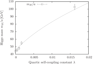
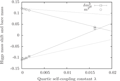
(a)	(b)

Figure 1: (a) The dependence of the Higgs boson mass $m_{H}/a$ on the quartic self-coupling constant $\lambda$ at $\Lambda=400\,\mbox{GeV}$ on a $16^{3}\times 32$-lattice for constant, degenerate Yukawa coupling constants fixed according to Eq. (20) and $N_{f}=1$. The prediction from the effective potential in Eq. (27) is represented by the dashed curve. (b) The corresponding Higgs boson mass shifts $\delta m_{H}^{2}$ and bare masses $m^{2}$ versus the quartic coupling constant $\lambda$. The dotted (dashed) lines show the analytical results derived from the unimproved (improved) effective potential.

Here, the momentum $p=0$ is excluded in the sum over the Goldstone loop, since the Goldstone propagator at zero momentum is identical to zero due to the rotation of the field $\varphi$ introduced in section II. However, with increasing lattice volume this exclusion looses any significance. The factors appearing in the nominators of Eq. (31) are given by the multiplicities of the considered diagrams. Though the effective potential $U[v]$ was actually given in bare constants, we plug the renormalized Higgs and Goldstone boson masses into the expressions for the scalar propagators, in order to further improve the result. For the evaluation of Eq. (31) independent of any knowledge from Monte-Carlo simulations we use $m_{Gp}=0$ in the following and determine $m_{Hp}$ self-consistently with respect to the curvature of the resulting improved effective potential at its minimum.

The results for the mass shifts and bare masses obtained by the improved effective potential are shown in Fig. 1b depicted by the dashed lines. The improved results are in very good agreement with the numerical data. The reason why the unimproved effective potential could describe the renormalized masses presented in Fig. 1a so well - in contrast to the bare masses and mass shifts - is, that the improvement term exactly cancels in Eq. (30) but not in the equation for the bare mass.

V Lower mass bounds

Given the knowledge about the $\lambda$-dependence of the renormalized Higgs boson mass we can now safely determine the cutoff-dependence of the lower Higgs boson mass bound by evaluating the Higgs boson mass at $\lambda=0$ for several values of $\Lambda$. Two restrictions limit the range of accessible energy scales: on the one side all particle masses have to be small compared to $\Lambda$ to avoid unacceptably large cutoff-effects, on the other side all masses have to be large compared to the inverse lattice size to avoid finite volume effects. As a minimal requirement we demand here that all particle masses $\hat{m}$ in lattice units fulfill

$$\hat{m}<0.5 \hat{m}\cdot L_{s,t}>2.$$ and (32)

For a lattice with side lengths $L_{s}=L_{t}=32$, a degenerate top/bottom quark mass of $175\,\mbox{GeV}$, and Higgs boson masses ranging from $40$ to $70$ GeV one can thus access energy scales $\Lambda$ from $350\,\mbox{GeV}$ to approximately $1100$ GeV.

In Fig. 2a we show the numerically obtained Higgs correlator masses $m_{H}/a$ versus the cutoff $\Lambda$. All presented results have been obtained in Monte-Carlo simulations with identical, degenerate bare Yukawa coupling constants fixed according to Eq. (20), $\lambda=0$, and $N_{f}=1$. To illustrate the influence of the finite lattice volume we have rerun all simulations with exactly the same parameter settings but different lattice sizes. Those results belonging to the same parameter sets are connected by dotted lines to guide the eye. Additionally, we also present the corresponding analytical, finite volume expectations for the cutoff-dependence of the Higgs boson mass as derived from the effective potential. We observe that the effective potential calculation is in very good agreement with the cutoff dependence of the measured Higgs boson masses. It also correctly predicts the observed finite volume effects.

The cutoff dependence of the corresponding top quark masses is presented in Fig. 2b. Those results belonging to the same bare parameters are connected by dotted lines for a better overview. The renormalized top quark mass, and thus the renormalized Yukawa coupling constant, decreases slightly with growing cutoff as expected in a trivial theory. In order to hold the fermion masses constant as desired one would have to fine-tune the bare Yukawa coupling parameters, giving rise to an additional but small contribution to the cutoff dependence of the Higgs boson mass.

For an efficient tuning of the bare Yukawa coupling constants, however, a thorough analytical understanding of the observed behaviour of the fermion mass would be indispensable. We therefore compare the presented numerical findings for the top quark mass to the corresponding 1-loop lattice perturbation theory predictions, depicted by the dashed lines in Fig. 2b and observe good agreement, allowing one ultimately to hold the fermion masses constant in follow-up Monte-Carlo calculations.

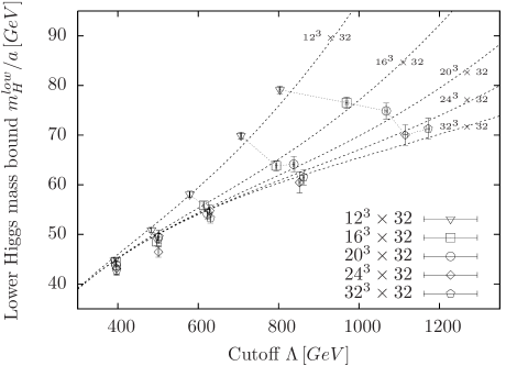
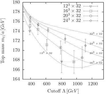
(a)	(b)

Figure 2: (a) The lower Higgs boson mass bound $m_{H}^{low}/a$ versus the cutoff $\Lambda$. (b) The cutoff dependence of the top quark mass $m_{t}/a$. To illustrate finite volume effects, simulations have been rerun with identical parameter sets but different lattice sizes. Runs with same parameter sets are connected via dotted lines to guide the eye. The analytical predictions for the respective lattice sizes derived from the effective potential are depicted by the dashed curves. All presented results have been obtained in Monte-Carlo simulations with identical, degenerate bare Yukawa coupling constants fixed according to Eq. (20), $\lambda=0$, and $N_{f}=1$.

The presented perturbative results are given by the tree-level fermion propagator plus the 1-Goldstone-loop and 1-Higgs-loop corrections according to

$$\left(\begin{array}[]{*{2}{c}}t\bar{t}(p)&\\ &b\bar{b}(p)\\ \end{array}\right) = \left[\tilde{D}(p)-\Sigma(p)\right]^{-1},\quad\tilde{D}(p)={\cal D}^{(ov)}(p)+v\cdot B_{0}\Gamma(p),$$ (35)

$$\Gamma(p) = \mathbbm{1}-\frac{1}{2\rho}{\cal D}^{(ov)}(p),\quad B_{\mu}=P_{+}\sigma^{\dagger}_{\mu}\mbox{diag}(y_{t},y_{b})+P_{-}\mbox{diag}(y_{t},y_{b})\sigma_{\mu},$$ (36)

$$\Sigma(p) = \frac{1}{L_{s}^{3}\cdot L_{t}}\cdot\sum\limits_{k\in{\cal P}}\frac{B_{0}\Gamma(k)\tilde{D}^{-1}(k)B_{0}\Gamma(p)}{\hat{t}^{2}+m^{2}_{Hp}}$$ (37)

$$+ \frac{1}{L_{s}^{3}\cdot L_{t}}\cdot\sum\limits_{p\neq k\in{\cal P}}\sum\limits_{i=1}^{3}\frac{B_{i}\Gamma(k)\tilde{D}^{-1}(k)B_{i}\Gamma(p)}{\hat{t}^{2}},\quad\mbox{with}\quad t=p-k.$$

Here $\hat{t}^{2}$ is the squared lattice momentum of the relative momentum $t=p-k$ as defined in Eq. (12) and ${\cal D}^{(ov)}(p)$ denotes the $8\times 8$ doublet Dirac matrix in momentum space for the given lattice momentum $p\in{\cal P}$. We remark that the contribution from the tadpole diagram to the fermion propagator is exactly canceled by the renormalization of the vev induced by the tadpole diagram. Again, the fact that the zero momentum mode of the Goldstone propagator is identical to zero due to the rotation of the field $\varphi$ as described in section II has to be respected by excluding these modes in the summation. From the 1-loop propagators $t\bar{t}(p)$ and $b\bar{b}(p)$ we calculate the top and bottom time-slice correlator as defined in Eq. (25) via a Fourier transformation in the time direction. The physical fermion masses shown in Fig. 2b are then determined from the exponential decay of this correlator.

From Fig. 2a one also learns that the finite volume effects are rather mild at $\Lambda=400\,\mbox{GeV}$ with $m_{H}\cdot L_{s,t}>3.2$ on the $32^{4}$-lattice, while the vev, and thus the associated cutoff $\Lambda$, as well as the Higgs boson mass itself vary strongly with increasing lattice size $L_{s}$ at the higher cutoffs. In Fig. 3 we explicitly show this volume dependence of the vev and the Higgs boson mass, respectively.

It is well known from investigations of pure $O(4)$ Higgs models Hasenfratz:1989ux ; Hasenfratz:1990fu ; Gockeler:1991ty that the vev as well as the mass receive strong contributions from the massless Goldstone modes, inducing finite volume effects starting at $O(L_{s}^{-2})$. The next non-trivial finite volume contribution was shown to be of order $O(L_{s}^{-4})$. In Fig. 3 we therefore plot the obtained data versus $1/L_{s}^{2}$ and use the linear fit ansatz

$$f^{(l)}_{v,m}(L_{s}^{-2})=A^{(l)}_{v,m}+B^{(l)}_{v,m}\cdot L_{s}^{-2}$$ (38)

to extrapolate to the infinite volume limit. The free fitting parameters $A^{(l)}_{v,m}$ and $B^{(l)}_{v,m}$ with the subscripts $v$ and $m$ refer to the renormalized vev $v_{r}$ and the Higgs boson mass $m_{H}$, respectively.

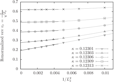
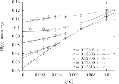
(a)	(b)

Figure 3: (a) The dependence of the renormalized vev $v_{r}=v/\sqrt{Z_{G}}$ on the squared inverse lattice side length $1/L^{2}_{s}$ for the same model parameters used in the Monte-Carlo runs presented in Fig. 2a but for a greater set of different lattice sizes. The given hopping parameters $\kappa$ are associated to cutoffs ranging from $\Lambda=400\,\mbox{GeV}$ to $\Lambda\approx 1200\,\mbox{GeV}$. (b) The dependence of the Higgs correlator mass $m_{H}$ versus $1/L^{2}_{s}$ for the same Monte-Carlo runs. The solid and dashed curves display the linear and parabolic fits as discussed in the main text.

To respect the presence of higher order terms in $1/L_{s}^{2}$ we include only the five largest lattice sizes in the linear fit. As a consistency check to test the dependence of these results on the choice of the fit ansatz, we furthermore consider the parabolic ansatz

$$f^{(p)}_{v,m}(L_{s}^{-2})=A^{(p)}_{v,m}+B^{(p)}_{v,m}\cdot L_{s}^{-2}+C^{(p)}_{v,m}\cdot L_{s}^{-4}$$ (39)

which we apply to the whole range of available lattice sizes. The deviation between the two fitting procedures are considered here as an additional systematic uncertainty for the infinite volume results determined from the linear fit in Eq. (38). The obtained fitting curves are displayed in Fig. 3a,b and the corresponding infinite volume extrapolations of the vev and the Higgs boson mass are listed in Tab. 1.

	Linear fit		Parabolic fit		Final result
$\kappa$	$A^{(l)}_{v}$	$A^{(l)}_{m}$	$A^{(p)}_{v}$	$A^{(p)}_{m}$	$v_{r}$	$m_{H}$
$\,0.12301\,$	$\,0.1947(15)\,$	$\,0.0535(20)\,$	$\,0.1918(24)\,$	$\,0.0517(15)\,$	$\,0.1947(15)(29)\,$	$\,0.0535(20)(18)\,$
$\,0.12303\,$	$\,0.2761(24)\,$	$\,0.0676(13)\,$	$\,0.2766(21)\,$	$\,0.0648(23)\,$	$\,0.2761(24)(05)\,$	$\,0.0676(13)(28)\,$
$\,0.12306\,$	$\,0.3860(10)\,$	$\,0.0826(15)\,$	$\,0.3882(73)\,$	$\,0.0825(14)\,$	$\,0.3860(10)(22)\,$	$\,0.0826(15)(01)\,$
$\,0.12309\,$	$\,0.4883(03)\,$	$\,0.0955(35)\,$	$\,0.4903(03)\,$	$\,0.0959(24)\,$	$\,0.4883(03)(20)\,$	$\,0.0955(35)(04)\,$
$\,0.12313\,$	$\,0.6191(02)\,$	$\,0.1063(11)\,$	$\,0.6204(04)\,$	$\,0.1090(17)\,$	$\,0.6191(02)(13)\,$	$\,0.1063(11)(27)\,$

Table 1: The results of the infinite volume extrapolation of the Monte-Carlo data for the renormalized vev $v_{r}$ and the Higgs boson mass $m_{H}$. The extrapolation was performed by applying the linear fit ansatz in Eq. (38) and the parabolic ansatz in Eq. (39) as described in the main text. The final results are taken from the linear fit. An additional, systematic uncertainty of the final results is specified in the second pair of brackets taken from the deviation between the linear and parabolic fit results.

So far, the presented results have been determined in the mass degenerate case, i.e. for $y_{t}=y_{b}$, which is easier to access numerically. This brings up the question of how the results are influenced when pushing the top-bottom mass splitting to its physical value, i.e. $m_{b}/m_{t}\approx 0.024$. From Eq. (26) one expects the Higgs boson mass shift $\delta m_{H}^{2}$ to grow quadratically with decreasing $y_{b}$ and that is exactly what is observed in Fig. 4b. Here, the bare top Yukawa coupling constant $y_{t}$, the quartic coupling parameter, and the cutoff are held constant, while $y_{b}$ is lowered to the physical ratio of $y_{b}/y_{t}$. The numerical data for the Higgs boson mass shift $\delta m_{H}^{2}$ are in excellent agreement with the predictions based on the effective potential, which are depicted by the dashed lines in Fig. 4b. However, the Higgs boson mass itself does not increase but decrease with decreasing $y_{b}$ as shown in Fig. 4a. This is because the first effect in the mass shift is over-compensated by the shift in the phase transition line, which is moved towards smaller bare Higgs boson masses $m$. This behaviour of the bare Higgs boson mass is demonstrated also in Fig. 4b, where the numerical findings for the bare mass are compared to the corresponding expectations from the effective potential. Again very good agreement between both approaches is observed.

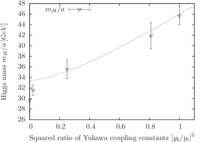
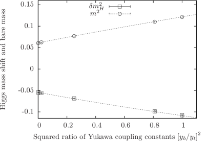
(a)	(b)

Figure 4: (a) The Higgs boson mass versus the squared ratio of the top and bottom Yukawa coupling constants $\left[y_{b}/y_{t}\right]^{2}$ on a $12^{3}\times 32$-lattice for constant cutoff $\Lambda=400\,\mbox{GeV}$, $\lambda=0$, $N_{f}=1$, and $y_{t}$ fixed according to Eq. (20). (b) The corresponding Higgs boson mass shifts $\delta m_{H}^{2}$ and bare masses $m^{2}$ versus $\left[y_{b}/y_{t}\right]^{2}$. The dashed curves represent the analytical predictions derived from the effective potential.

Finally, we present the analytical infinite volume results, which are obtained from the effective potential in Eq. (31) by replacing the sums with corresponding integrals. In Fig. 5 we compare these findings to the infinite volume extrapolation of the Monte-Carlo data taken from Tab. 1 and observe very good agreement. We also show the analytical infinite volume expectations for several other physical scenarios with varying values for $N_{f}$ and $y_{b}/y_{t}$ to study the influence of these parameters on the lower mass bound. The number of fermion generations (or here equivalently the number of colours) as well as the bottom-top mass splitting have a strong impact on the lower mass bound. The solid curve in Fig. 5 with $N_{f}=3$ and $y_{b}/y_{t}=0.024$ comes closest to the actual situation in the Standard Model. However, direct Monte-Carlo simulations in this scenario on sufficiently large lattices would be too demanding with our available resources due to the huge mass splitting between the top and bottom quark.

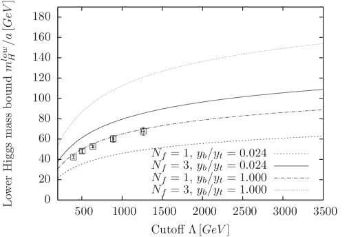
Figure 5: The various curves show the cutoff dependence of the lower Higgs boson mass bound in the infinite volume limit derived from the effective potential for different physical setups ($N_{f},y_{b}/y_{t}$). These analytical findings are compared with the infinite volume extrapolation of the Monte-Carlo data taken from Tab. 1 depicted by the square symbols. The numerical results were obtained at ($N_{f}=1,y_{b}/y_{t}=1$) and are in very good agreement with the corresponding dash-dotted curve. The solid curve represents the setup ($N_{f}=3,y_{b}/y_{t}=0.024$) coming closest to the actual physical situation in the Standard Model.

VI Outlook towards upper Higgs boson mass bounds

We now turn towards the determination of the upper Higgs boson mass bound $m_{H}^{up}(\Lambda)$. First, we investigate whether the largest Higgs boson masses are obtained at $\lambda=\infty$ as expected from perturbation theory. This can indeed be observed in Fig. 6a where we plot the physical Higgs boson mass $m_{H}/a$ versus the quartic self-coupling constant in the strong coupling region of the model for a fixed cutoff $\Lambda\approx 1500\,\mbox{GeV}$. We compare these numerical findings for large but finite $\lambda$ with the corresponding $\lambda=\infty$ result, which was obtained from our Monte-Carlo simulations by reparametrizing the Higgs field $\phi_{x}$ in terms of $SU(2)$ elements. Since the integration of the molecular dynamics equations as needed in our Monte-Carlo algorithm becomes increasingly difficult with growing $\lambda$, we present here only a few results on rather small $12^{3}\times 32$-lattices. However, within the available accuracy one can conclude from Fig. 6a that the largest Higgs boson masses are obtained at $\lambda=\infty$, as expected. We therefore derive the upper Higgs boson mass bounds in the following from simulations with infinite self-coupling constant.

As discussed in the previous section the accessible energy scales $\Lambda$ are restricted by Eq. (32). Employing a top mass of $175\,\mbox{GeV}$ and a Higgs boson mass of below $700\,\mbox{GeV}$, as suggested by Fig. 6c, we should be able to reach cutoffs between $1400\,\mbox{GeV}$ and $2100\,\mbox{GeV}$ on a $24^{3}\times 32$-lattice.

In Fig. 6b we present the results for the top quark mass obtained in our Monte-Carlo calculations with degenerate bare Yukawa coupling constants fixed according to Eq. (20) and $N_{f}=1$. Again we estimate the strength of the finite volume effects by rerunning the simulations on different lattice sizes. One sees that for the simulation runs with $\Lambda<2.1\,\mbox{TeV}$ the volume dependence of the top quark mass has already reached its saturation plateau on the $24^{3}\times 32$-lattices within the given accuracy. In comparison to the weak coupling region of the model the top quark mass depends significantly weaker on the cutoff. The discrepancy between the tree-level determination of the bare Yukawa coupling constants and the targeted top quark mass is around $1\%$ for the largest presented lattices and thus smaller than in the weak coupling region. However, in follow-up calculations the available data can be used for a fine tuning of the bare Yukawa coupling constants to reproduce the targeted fermion masses even more precisely.

Finally, we present our results on the cutoff dependence of the upper Higgs boson mass bound in Fig. 6c. Here, we decided to show only the propagator masses instead of the correlator masses. The reason is that the latter results are very noisy, since they are based on only those $L_{t}$ Higgs modes in momentum space which have spatial momentum zero, and do - at the time being - not allow for a clear observation of the cutoff dependence of the Higgs boson mass. The propagator masses, on the other hand, are much more stable and do reveal the desired cutoff dependence of the upper mass bound. On the small $12^{3}\times 32$-lattices the Higgs boson mass seems to increase with the cutoff $\Lambda$. This, however, is only a finite volume effect. On the larger lattices the Higgs boson mass decreases with growing $\Lambda$ as expected. Only when the cutoff becomes too high for the given lattice volume does the Higgs boson mass finally start increasing again due to the finite volume. Larger lattice sizes and more statistics are needed here to further follow the cutoff dependence of the upper mass bound.

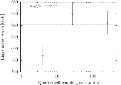
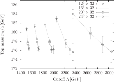
(a)        (b)

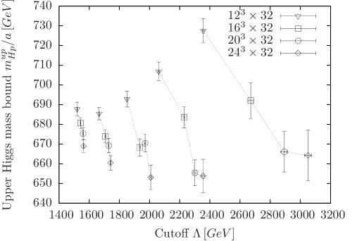
(c)

Figure 6: (a) The correlator Higgs boson mass versus the quartic coupling constant $\lambda$ in the strong coupling region of the model at $\Lambda\approx 1500\,\mbox{GeV}$ on a $12^{3}\times 32$-lattice. The dashed line depicts the corresponding $\lambda=\infty$ result. (b) The cutoff dependence of the top correlator mass at $\lambda=\infty$. (c) The cutoff dependence of the Higgs propagator mass at $\lambda=\infty$. Finite volume effects are illustrated in panels b, c by rerunning the simulations on several lattice sizes. Runs with identical bare parameter settings are connected by lines to guide the eye. All presented results have been obtained in Monte-Carlo simulations with identical, degenerate bare Yukawa coupling constants fixed according to Eq. (20) and $N_{f}=1$.

VII Summary and outlook

The eventual aim of our work is to establish non-perturbative upper and lower Higgs boson mass bounds based on first principle computations without relying on arguments such as vacuum instability or triviality. This can be achieved by investigating a lattice model of the pure Higgs-Yukawa sector of the Standard Model. The main idea of this approach is to apply direct Monte-Carlo simulations to determine the maximal interval of Higgs boson masses attainable within this model being consistent with phenomenology, i.e. with the physical values of the top and bottom quark masses and the vacuum expectation value of the Higgs mode. To maintain the chiral character of the Higgs-fermion coupling structure on the lattice we have considered here a chirally invariant lattice Higgs-Yukawa model based on the Neuberger Dirac operator.

In the present paper we confirmed that the lightest Higgs boson masses are generated at vanishing quartic self-coupling, as expected from perturbation theory. For the mass degenerate case with equal top and bottom quark masses and $N_{f}=1$ we presented our numerical data for the Higgs boson mass obtained at $\lambda=0$ for various cutoffs and lattice sizes. These results were compared to the analytical calculations of the Higgs boson mass based on the effective potential at one-loop order. We then extrapolated the numerical finite size results to infinite volume and compared them to the corresponding infinite volume effective potential predictions. In both cases very good agreement was observed.

The main result of the presented findings is that a lower Higgs boson mass bound is a manifest property of the pure Higgs-Yukawa sector that evolves directly from the Higgs-fermion interaction for a given Yukawa coupling parameter. For growing cutoff this lower mass constraint rises monotonically with flattening slope as expected from perturbation theory. Moreover, the quantitative size of the lower bound is comparable to the magnitude of the perturbative results based on vacuum stability considerations Hagiwara:2002fs . A direct quantitative comparison is, however, non-trivial due to the different regularization schemes accompanied with the strong cutoff dependence of the considered constraints.

We also studied the Higgs boson mass dependence on the top-bottom mass splitting on some smaller lattices, where the calculations were feasible. Again the numerical findings matched the corresponding results based on the effective potential. The very good agreement between the numerical and analytical approaches justifies the presented effective potential calculations performed in the actual physical situation with $N_{f}=3$ and $m_{t}/m_{b}\approx 40$. A comparison with direct Monte-Carlo simulations in that setup on sufficiently large lattice sizes, however, seems to be too demanding for our available resources at the moment. We therefore have to rely on the analytical results in this case for the time being.

Additionally, we turned towards the upper Higgs boson mass bound, which was obtained at infinite bare self-coupling after having checked that the heaviest Higgs boson masses are indeed generated at $\lambda=\infty$ as expected. Instead of the correlator masses we decided to present the propagator masses at this point, since the latter results were stable enough to allow for the observation of the desired cutoff dependence of the upper Higgs boson mass bound in contrast to the correlator masses. Apart from finite volume effects the expected decrease of the upper bound with growing cutoff could clearly be seen.

As a next step we will improve the statistics for the upper Higgs boson mass bound, extend the lattice volumes, and compare the numerical findings to corresponding calculations in renormalized perturbation theory, once sufficient precision is achieved. For the lower bound we plan to include higher order terms into the bare Lagrangian in order to investigate the universality of the obtained results. Taking these future improvements aside, our present results suggest a maximally allowed Higgs boson mass interval of $80\mathrm{Gev}\lesssim m_{H}\lesssim 700\mathrm{Gev}$ at a cutoff around $\Lambda\approx 1\,\mbox{TeV}$. Eventually, we are also interested in studying the decay properties of the Higgs boson with this lattice model.

References

- (1) M. Aizenman. Proof of the Triviality of phi**4 in D-Dimensions Field Theory and Some Mean Field Features of Ising Models for D. Phys. Rev. Lett. 47:1–4, 1981.
- (2) J. Fröhlich. On the Triviality of Lambda (phi**4) in D-Dimensions Theories and the Approach to the Critical Point in D Four-Dimensions. Nucl. Phys. B200:281–296, 1982.
- (3) M. Lüscher and P. Weisz. Scaling Laws and Triviality Bounds in the Lattice phi**4 Theory. 3. N Component Model. Nucl. Phys. B318:705, 1989.
- (4) A. Hasenfratz, K. Jansen, C. B. Lang, Thomas Neuhaus, and Hiroshi Yoneyama. The Triviality Bound of the Four Component phi**4 Model. Phys. Lett. B199:531, 1987.
- (5) J. Kuti, L. Lin, and Y. Shen. Upper Bound on the Higgs Mass in the Standard Model. Phys. Rev. Lett. 61:678, 1988.
- (6) A. Hasenfratz et al. Study of the Four Component phi**4 Model. Nucl. Phys. B317:81, 1989.
- (7) M. Göckeler, H A. Kastrup, T. Neuhaus, and F. Zimmermann. Scaling analysis of the 0(4) symmetric Phi**4 theory in the broken phase. Nucl. Phys. B404:517–555, 1993.
- (8) N. Cabibbo, L. Maiani, G. Parisi, and R. Petronzio. Bounds on the Fermions and Higgs Boson Masses in Grand Unified Theories. Nucl. Phys. B158:295, 1979.
- (9) R. F. Dashen and H. Neuberger. How to Get an Upper Bound on the Higgs Mass. Phys. Rev. Lett. 50:1897, 1983.
- (10) M. Lindner. Implications of Triviality for the Standard Model. Zeit. Phys. C31:295, 1986.
- (11) D. A. Dicus and V. S. Mathur. Upper bounds on the values of masses in unified gauge theories. Phys. Rev. D7:3111–3114, 1973.
- (12) B. W. Lee, C. Quigg, and H. B. Thacker. Weak Interactions at Very High-Energies: The Role of the Higgs Boson Mass. Phys. Rev. D16:1519, 1977.
- (13) W. J. Marciano, G. Valencia, and S. Willenbrock. Renormalization group improved unitarity bounds on the Higgs boson and top quark masses. Phys. Rev. D40:1725, 1989.
- (14) A. D. Linde. Dynamical Symmetry Restoration and Constraints on Masses and Coupling Constants in Gauge Theories. JETP Lett. 23:64–67, 1976.
- (15) S. Weinberg. Mass of the Higgs Boson. Phys. Rev. Lett. 36:294–296, 1976.
- (16) A. D. Linde. On the Vacuum Instability and the Higgs Meson Mass. Phys. Lett. B70:306, 1977.
- (17) M. Sher. Electroweak Higgs Potentials and Vacuum Stability. Phys. Rept. 179:273–418, 1989.
- (18) M. Lindner, M. Sher, and H. W. Zaglauer. Probing Vacuum Stability Bounds at the Fermilab Collider. Phys. Lett. B228:139, 1989.
- (19) K. Hagiwara et al. Review of particle physics. Phys. Rev. D66:010001, 2002.
- (20) L. O’Raifeartaigh, A. Wipf, and H. Yoneyama. The constraint effective potential. Nucl. Phys. B271:653, 1986.
- (21) K. Holland and J. Kuti. How light can the Higgs be. Nucl. Phys. Proc. Suppl. 129:765–767, 2004.
- (22) K. Holland. Triviality and the Higgs mass lower bound. Nucl. Phys. Proc. Suppl. 140:155–161, 2005.
- (23) G. Bhanot, K. Bitar, U. M. Heller, and H. Neuberger. Phi**4 on F(4): Numerical results. Nucl. Phys. B353:551–564, 1991.
- (24) M. Göckeler, H. A. Kastrup, J. Westphalen, and F. Zimmermann. Scattering phases on finite lattices in the broken phase of the four-dimensional O(4) phi**4 theory. Nucl. Phys. B425:413–448, 1994.
- (25) J. Smit. Standard model and chiral gauge theories on the lattice. Nucl. Phys. Proc. Suppl. 17:3–16, 1990.
- (26) J. Shigemitsu. Higgs-Yukawa chiral models. Nucl. Phys. Proc. Suppl. 20:515–527, 1991.
- (27) M. F. L. Golterman. Lattice chiral gauge theories: Results and problems. Nucl. Phys. Proc. Suppl. 20:528–541, 1991.
- (28) A. K. De and J. Jersák. Yukawa models on the lattice. HLRZ Jülich, HLRZ 91-83, preprint edition, 1991.
- (29) I. Montvay and G. Münster. Quantum Fields on a Lattice (Cambridge Monographs on Mathematical Physics). Cambridge University Press, 1997.
- (30) M. F. L. Golterman, D. N. Petcher, and E. Rivas. On the Eichten-Preskill proposal for lattice chiral gauge theories. Nucl. Phys. Proc. Suppl. 29BC:193–199, 1992.
- (31) K. Jansen. Domain wall fermions and chiral gauge theories. Phys. Rept. 273:1–54, 1996.
- (32) M. Lüscher. Exact chiral symmetry on the lattice and the Ginsparg- Wilson relation. Phys. Lett. B428:342–345, 1998.
- (33) P. H. Ginsparg and K. G. Wilson. A remnant of chiral symmetry on the lattice. Phys. Rev. D25:2649, 1982.
- (34) P. Gerhold and K. Jansen. The phase structure of a chirally invariant lattice Higgs-Yukawa model for small and for large values of the Yukawa coupling constant. JHEP 09:041, 2007.
- (35) P. Gerhold and K. Jansen. The phase structure of a chirally invariant lattice Higgs-Yukawa model - numerical simulations. JHEP 10:001, 2007.
- (36) Z. Fodor, K. Holland, J. Kuti, D. Nogradi, and C. Schroeder. New Higgs physics from the lattice. PoS LAT2007:056, 2007.
- (37) P. Gerhold and K. Jansen. The phase structure of a chirally invariant lattice Higgs-Yukawa model. PoS LAT2007:075, 2007.
- (38) A. Hasenfratz, W. Liu, and T. Neuhaus. Phase structure and critical points in a scalar fermion model. Phys. Lett. B236:339, 1990.
- (39) I.-H. Lee, J. Shigemitsu, and R. E. Shrock. Study of different lattice formulations of a Yukawa model with a real scalar field. Nucl. Phys. B334:265, 1990.
- (40) W. Bock et al. Phase diagram of a lattice SU(2) x SU(2) scalar fermion model with naive and Wilson fermions. Nucl. Phys. B344:207–237, 1990.
- (41) L. Lin, I. Montvay, and H. Wittig. Phase structure of a U(1)-L x U(1)-R symmetric Yukawa model. Phys. Lett. B264:407–414, 1991.
- (42) A. Hasenfratz, P. Hasenfratz, K. Jansen, J. Kuti, and Y. Shen. The Equivalence of the top quark condensate and the elementary Higgs field. Nucl. Phys. B365:79–97, 1991.
- (43) A. Hasenfratz, K. Jansen, and Y. Shen. The Phase diagram of a (1) Higgs-Yukawa model at finite lambda. Nucl. Phys. B394:527–540, 1993.
- (44) W. Bock, J. Smit, and J. C. Vink. Fermion Higgs model with reduced staggered fermions. Phys. Lett. B291:297–305, 1992.
- (45) W. Bock, M. F. L. Golterman, and Y. Shamir. On the phase diagram of a lattice U(1) gauge theory with gauge fixing. Phys. Rev. D58:054506, 1998.
- (46) W. Bock, K. C. Leung, M. F. L. Golterman, and Y. Shamir. The phase diagram and spectrum of gauge-fixed Abelian lattice gauge theory. Phys. Rev. D62:034507, 2000.
- (47) H. Neuberger. More about exactly massless quarks on the lattice. Phys. Lett. B427:353–355, 1998.
- (48) A. Hasenfratz et al. Finite size effects and spontaneously broken symmetries: The case of the 0(4) model. Z. Phys. C46:257, 1990.
- (49) A. Hasenfratz et al. Goldstone bosons and finite size effects: A Numerical study of the O(4) model. Nucl. Phys. B356:332–366, 1991.
- (50) M. Göckeler and H. Leutwyler. Constraint correlation functions in the O(N) model. Nucl. Phys. B361:392–414, 1991.
- (51) R. Frezzotti and K. Jansen. A polynomial hybrid Monte Carlo algorithm. Phys. Lett. B402:328–334, 1997.
- (52) R. Frezzotti and K. Jansen. The PHMC algorithm for simulations of dynamical fermions. I: Description and properties. Nucl. Phys. B555:395–431, 1999.
- (53) R. Frezzotti and K. Jansen. The PHMC algorithm for simulations of dynamical fermions. II: Performance analysis. Nucl. Phys. B555:432–453, 1999.
- (54) M. Frigo and S. G. Johnson. The design and implementation of FFTW3. Proceedings of the IEEE 93(2):216–231, 2005. special issue on ”Program Generation, Optimization, and Platform Adaptation”.
- (55) G. G. Batrouni et al. Langevin Simulations of Lattice Field Theories. Phys. Rev. D32:2736, 1985.
- (56) G. Parisi. Progress in Gauge Field Theory, page 531. World Scientific, Singapore, 1984.
- (57) S. R. Coleman and E. J. Weinberg. Radiative Corrections as the Origin of Spontaneous Symmetry Breaking. Phys. Rev. D7:1888–1910, 1973.