A large-scale CO survey of the Rosette Molecular Cloud: assessing the effects of O stars on surrounding molecular gas

Abstract

We present a new large-scale survey of the J=3–2 ¹²CO emission covering 4.8 square degrees around the Rosette Nebula. The results reveal the complex dynamics of the molecular gas in this region. We identify about 2000 compact gas clumps having a mass distribution given by $dN/dM\sim M^{-1.8}$, with no dependence of the power law index on distance from the central O stars. A detailed study of a number of the clumps in the inner region show that most exhibit velocity gradients in the range 1–3 $kms^{-1}pc^{-1}$, generally directed away from the exciting nebula. The magnitude of the velocity gradient decreases with distance from the central O stars, and we compare the apparent clump acceleration with a photoionised gas acceleration model. For most clumps outside the central nebula, the model predicts lifetimes of a few $10^{5}yrs$. In one of the most extended of these clumps, however, a near-constant velocity gradient can be measured over 1.7 pc, which is difficult to explain with radiatively-driven models of clump acceleration.

As well as the individual accelerated clumps, an unresolved limb-brightened rim lies at the interface between the central nebular cavity and the Rosette Molecular Cloud. Extending over 4 pc along the edge of the nebula, this region is thought to be at earlier phase of disruption than the accelerating compact globules.

Blue-shifted gas clumps around the nebula are in all cases associated with dark absorbing optical globules, indicating that this material lies in front of the nebula and has been accelerated towards us. Red-shifted gas shows little evidence of associated line-of-sight dark clouds, indicating that the dominant bulk molecular gas motion throughout the region is expansion away from the O stars. In addition, we find evidence that many of the clumps lie in a molecular ring, having an expansion velocity of 30 km$s^{-1}$ and radius 11 pc. The dynamical timescale derived for this structure – $\sim 10^{6}yrs$ – is similar to the age of the nebula as a whole ($2\times 10^{6}yrs$).

The J=3-2/1-0 ¹²CO line ratio in the clumps decreases with radial distance from the exciting O stars, from 1.6 at $\sim$8 pc distance, to 0.8 at 20pc. This can be explained by a gradient in the surface temperature of the clumps with distance, and we compare the results with a simple model of surface heating by the central luminous stars.

We identify 7 high-velocity molecular flows in the region, with a close correspondence between these flows and embedded young clusters or known young luminous stars. These flows are sufficiently energetic to drive gas turbulence within each cluster, but fall short of the turbulent energy of the whole GMC by two orders of magnitude.

We find 14 clear examples of association between an embedded young star (as seen by Spitzer at 24$\mu m$) and a CO clump in the molecular cloud facing the nebular. The CO morphology indicates that these are photo-evaporating circumstellar envelopes. CO clumps without evidence of embedded stars tend to have lower gas velocity gradients. It is suggested that the presence of the young star may extend the lifespan of the externally-photoevaporating envelope.

1 Introduction

It is likely that a significant fraction of all solar-type stars formed in molecular clouds in the vicinity of massive luminous stars (eg Hester & Desch, 2005). An understanding of the interaction between OB stars and their molecular gas environment is therefore necessary in order to understand star formation. Such interaction has been the subject of considerable theoretical study (eg Bertoldi & McKee, 1990), and hydrodynamic models show that complex dynamic structures are formed in such environments (eg Lefloch & Lazareff, 1994). But the effects of OB stars on the formation of new lower-mass stars remains unclear: both modest enhancements (eg Dale et al., 2007) and supression of the star formation rate (eg McKee, 1989) have been suggested. Over the complete lifespan of a Giant Molecular Cloud however, the presence of OB stars does limit the star formation efficiency, due to the eventual dispersal of the molecular gas by ionising stellar photons and winds (eg McKee & Ostriker, 2007). The interaction between OB stars and GMCs have clear observational signatures, including ionisation fronts, Photon Dominated Regions (PDRs), bright-rimmed clouds, dark clumps and cometary globules (eg Hester et al., 1996). However, optical and infrared observations of dark clouds and globules reveal only part of the picture; they show neither the internal structure nor the dynamics of the absorbing clouds, and they can only be seen in the foreground of diffuse emission nebulae.

The Rosette Nebula, by dint of its overall symmetry and simple optical morphology, has long been regarded as a textbook example of the interaction between OB stars and surrounding gas. The central cluster (NGC 2244) contains six O stars with a total luminosity of $\sim 10^{6}L_{\odot}$ (Celnik 1985). Surrounding these is the well-known symmetrical optical emission nebula. To the southeast lies a large molecular cloud complex, known as the Rosette Molecular Cloud (hereafter “RMC”), of total mass $10^{5}M_{\odot}$, and extent $\sim$40pc (eg Williams et al., 1995 - W95). Near the centre of the RMC lies the luminous embedded star AFGL961, well studied because of its bright infrared spectra and outflow signatures (eg Lada & Gautier, 1982). The RMC itself has been mapped in the J=1-0 transitions of ¹²CO and ¹³CO, with spatial resolutions of 8 arcmin (Blitz & Thaddeus, 1980), 1.7 arcmin (Blitz & Stark, 1986) and 45 arcsec (Heyer et al., 2006). More detailed studies have also been undertaken of individual objects within the RMC (eg Patel et al., 1993; Schneider et al., 1998).

In the present work we describe new large-scale observations of the Rosette Nebula and the surrounding region obtained with high spatial resolution (14 arcsec) in the J=3-2 transition of ¹²CO. This transition has an upper energy level of 33K and critical density of $10^{4}cm^{-3}$, as compared to 13K and $300cm^{-3}$ for the 1-0 transition, and so are sensitive to relatively compact, warm clumps of dense gas. We use the data to take a census of outflows within the RMC (section 3.1), look at the overall spatial and velocity structure of the gas (3.2), and investigate the compact clumps (3.3). We compare the results with published CO 1–0 data as well as observations of embedded young stars, in order to determine the effects of the Rosette O-stars on the surrounding GMC. We have adopted a distance of 1400 pc for the Rosette Nebula (Hensberge et al., 2000).

2 Observations

The observations described in this paper were carried out using the newly-commissioned heterodyne receiver array installed on the James Clerk Maxwell Telescope, Mauna Kea, Hawaii. The system consists of HARP, the 16-element frontend receiver (Smith et al., 2003), and ACSIS, the backend correlator and data reduction system (Hovey et al., 2000). Controlling these instruments, as well as the telescope, is a hardware realtime sequencer, as well as a high-level software control system, known as the OCS (Rees et al., 2002). For an overall description, see Hills et al. (2008).

The large datacubes in the present observations were obtained using the fast raster-scan observing mode of ACSIS/HARP. The telescope was scanned at 75 arcsec/second with a 10 Hz sampling rate, providing 7.5 arcsec sampling in the scan direction. The orientation of the regular square array of the HARP frontend was maintained at $13\mbox{\,${}^{\circ}$}$ to the scan direction using a mechanical beam rotator; with the diffraction-limited beam size of 14 arcsec and the HARP beam separation of 30 arcsec, this resulted in near Nyquist-sampled data. The chosen sampling was found to provide a good compromise between wide area coverage and near Nyquist sampling of the sky. The final image was constructed from several map scans, typically $1\times 0.5\mbox{\,${}^{\circ}$}$ or $1\times 1\mbox{\,${}^{\circ}$}$ in extent, each requiring 30-60 minutes to complete (including pointing and observations of a spectral line standard). In most of the mapped region, a basket-weaving technique was employed, where the same area of sky was scanned in orthogonal directions (RA and Decl., J2000). To improve the signal to noise ratio, a second pair of orthogonal scans were made in some regions of the map. During most of the observations, two of the mixers were unusable and were flagged out during data reduction. The basket-weaving observing technique significantly improved the fidelity of the final images in such circumstances, by providing relatively even sky coverage, better redundancy, and reduced scanning artifacts. A common reference observation was taken every 60-100 seconds, at the end of every one or two rows. The line-free reference position used was $06^{h}35^{m}10.0^{s},+5\mbox{\,${}^{\circ}$}23\arcmin 32.7\arcsec$ (J2000; these are the coordinates of the array centre).

A total of 20 hours of observations were taken in 2006 Dec 9 and 15 and 2007 Feb 14 and 15, including calibration and pointing. System temperatures were mostly in the range 180-320K (SSB) during the runs (although one scan was done at low elevation, resulting in system temperatures as high as 450K). Main beam efficiency was determined to be 0.55$\pm 0.05$, as measured on Jupiter (size 30 arcsec) and the JCMT spectral line standard NGC2071IR. Measurements on the full Moon showed maximum mixer-to-mixer calibration differences of about 5% (Hills et al., 2009). The pointing errors of the telescope at the time of these observations were higher than normal, at 3 arcsec rms, as measured from observations of the nearby source NGC2071. However, the largest variation measured at the start and end of an individual raster map was 7 arcsec, significantly less than the beam size (14 arcsec), and hence these errors should not significantly affect the final map.

The ¹²CO J=3-2 line was observed in the lower sideband, at a rest frequency of 345.796GHz. ACSIS was set up in a configuration with a total of 1.0 GHz bandwidth per mixer; with 2048 spectral channels per IF and Natural weighting of the correlation function this resulted in an effective spectral resolution of 0.45$kms^{-1}$. The data were reduced and calibrated in real time using the ACSIS reduction software, which produces a time- and coordinate-stamped series of spectra. The Starlink SMURF package (Jenness et al., 2008) was used to transform these data into spectral cubes, using a 7.5 arcsec grid spacing and assigning each data sample to its´ nearest neighbour in the final cube. The Starlink KAPPA and CCDPACK routines were used to remove a linear baseline from each spectrum, transform to the same regular coordinate grid, and combine the maps into a single output data cube. To limit the final datacube size, only the central 66 spectral channels (from $v_{lsr}=-2.9$ to $25.1kms^{-1}$) were included.

Individual spectra in the unsmoothed datacube had noise levels ranging from 0.9 - 3.6 K (T_mb, rms). Moreover, because of the missing mixers, a small number of pixels in this datacube were not filled. To improve the fidelity of the images, the data were smoothed in the spatial dimensions by a Gaussian of width (fwhm) 15 arcsec, resulting in an effective image spatial resolution of 20 arcsec. The spectral rms noise per pixel in the final smoothed datacube then ranged from 0.2 - 0.5 K, with a mean value of 0.3 K (T_mb). The final map, of size $\sim 2\times 2.5\mbox{\,${}^{\circ}$}$, contained $10^{6}$ spectra.

3 Results

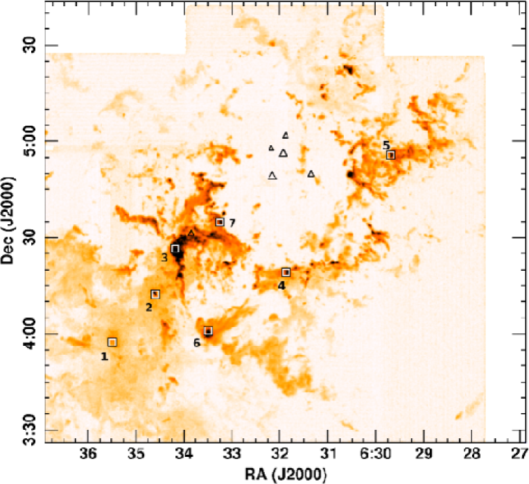
Figure 1: Image of peak ¹²CO J=3-2 emission from the region of the Rosette Nebula. O stars illuminating the optical nebula are shown as triangles, whose size represents their UV excitation parameter (values from Celnik, 1985). Squares show the locations and identification number of the outflows found in the region (see section 3.1 and Table 1). The CO greyscale ranges from 0 - 22 K (T_mb), and the image size is 2.5x2.5 degrees (60x60 pc).

An image of the peak CO J=3–2 emission, illustrating the overall structure of the warm molecular gas in the region, is displayed in Figure 1. Also shown are the locations of the O stars illuminating the Rosette optical nebula; the size of the symbols represents the UV excitation parameters of these stars (proportional to the radii of their Strömgren spheres - Celnik, 1985). This figure illustrates the lack of molecular gas in the central region around the most luminous O stars. The Rosette Molecular Cloud, previously mapped at lower angular resolution in the CO 1–0 transition (Blitz & Stark, 1986; Heyer et al., 2006) and (in part) in the 3–2 transition (Schneider et al., 1998), appears as the relatively bright complex structure to the SE of the O-star cluster, extending over about $1\mbox{\,${}^{\circ}$}$ (20pc). In the area of overlap, the new data agree reasonably well with the lower-resolution large-scale images of Heyer et al. (2006). However, the factor of $\sim 3$ higher resolution and the higher energy level of the J=3–2 CO transition reveals more clearly the complex small-scale structures in the warm gas throughout the cloud. In particular, many compact clumps are clearly seen surrounding the OB cluster and, by studying the full datacube, several high-velocity outflows are found in the region (see sections below). The peak brightness temperature shown in Fig. 1 emphasises the multiple compact (as well as some more extended) clouds with narrow, bright emission lines. The image also shows that many of the clumps and clouds are limb-brightening on their edge facing the O stars.

By consideration of the full datacube, we identify three distinct spatio-velocity structures: (1) relatively compact regions with broad line wings, identified as compact or well-collimated high-velocity flows, frequently associated with bright IRAS sources; (2) bright, compact clumps of emission, of sizes up to $\sim$3 arcmin ($\sim$1pc), many of which have significant velocity gradients; and (3) extensive undifferentiated regions of emission with narrow linewidths. The latter extended components were identified as ambient, relatively-undisturbed cool gas clouds in the region (Heyer et al., 2006). In the following sections we investigate the first two types of compact structures in more detail.

3.1 High-velocity outflows

Inspection of the full datacube reveal seven potential high-velocity (HV) protostellar outflows in the region; their locations and identifications are marked by squares on Figure 1. Such flows are identified in several ways. Firstly their line profiles show broad wings of emission extending $\geq 5kms^{-1}$ from the core cloud velocity, with a gradual decrease of intensity to higher relative velocities. This is substantially different in character from the discrete, narrow velocity components that would arise from clumps of ambient gas along the line-of-sight. As noted by Borkin et al. (2008), inspection of full position-velocity datacubes can rapidly reveal these regions of HV gas in complex regions. A confirmation of the HV outflow nature comes from the J=3–2 to J=1–0 line ratio in the wings. In all cases, this is significantly higher than the line core, implying that the HV gas is relatively warm. Finally, the regions of HV gas are spatially relatively compact, no larger than a few arcminutes, which is unlikely for multiple line-of-sight clumps.

Table 1 gives the characteristics of these regions of HV gas, and the CO J=3–2 spectral profiles at the central positions of the outflows are shown in Figure 2. We also include in Fig. 2 the CO J=1–0 profiles for comparison, using data taken by Heyer et al. (2006). The J=3–2 data have been smoothed to the same spatial resolution as that of the lower transition (45 arcsec) and both lines are shown on the main-beam brightness temperature scale, T_mb. In all cases, the line ratio in the wings lies in the range 1.5 – 3, indicating excitation temperatures of 40-60 K, assuming optically thin gas in LTE (cf Figure 12 below). To illustrate the spatio-velocity structure in the outflows, Figures 3 and 4 show position-velocity cuts through the objects. These reveal the notable differences in characteristics of the ambient clumpy gas (often extended in the spatial direction, but compact in the spectral dimension), and the outflow gas (spatially-compact, but with high-velocity wings). Further searches through the datacube revealed no other regions with similar characteristics, although it is possible that some are hidden by multiple narrow line components along some lines of sight.

Blitz & Stark (1986) proposed that broad CO emission from the RMC may be caused by high-velocity interclump gas. Conversely, Schneider et al. (1996) suggested that some of the apparent HV emission is actually due to the superposition of multiple line-of-sight clumps. The higher spatial resolution of the present data supports their origin in HV outflows, at least for the seven objects noted above. In Section 3.2, we discuss more the velocity extent of the compact clumps.

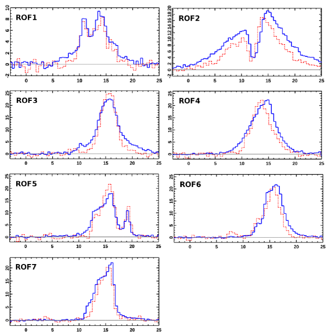
Figure 2: Spectra at the centres of the high-velocity flows identified in the region (ROF1-7); basic flow parameters are given in Table 1. The solid blue histograms show the J=3-2 ¹²CO line, and the dashed red histograms are J=1-0 data taken from Heyer et al. (2005). The J=3-2 data has been smoothed to the same spatial resolution as the lower transition (45 arcsec), and the intensities are given on the T_mb scale. Note that the spectrum of ROF2 extends beyond the velocity region shown; these data were used to remove the DC baseline offset, but were not included in the final datacube.

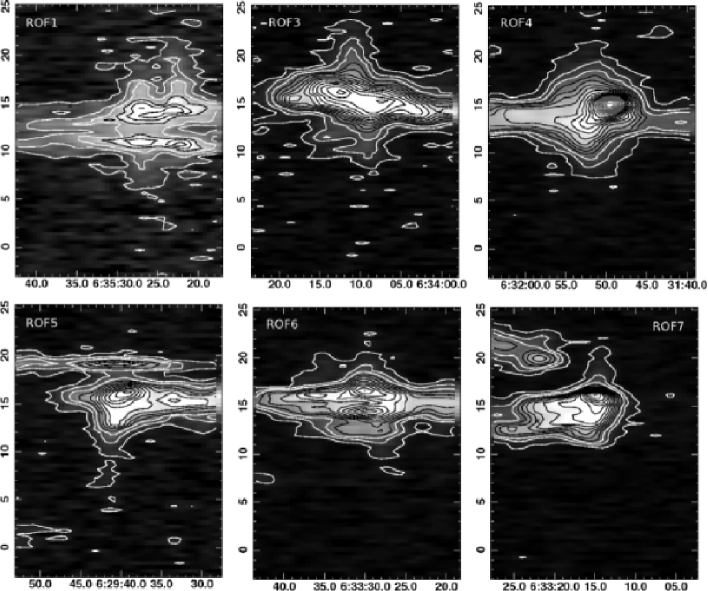
Figure 3: Position-velocity cuts through the Rosette outflows ROF1 and ROF3-7. ROF2 has a more complex structure, and is shown in Figure 4. The x-axes are RA, and the y-axes are velocity (lsr). Lowest contours are 1 K, with a contour interval of 2 K (T_mb). In all except ROF1, the centre of the cut corresponds to the coordinates in Table 1. For ROF1, the cut was through the peak HV emission to the SE of the centre (cf Figure 6).

Table 1: Parameters of molecular outflows detected in the Rosette field. See text for details.

Name	RA	Dec	IRAS	Cluster	Outflow	Max. extent	Integ. flux	Mass	KEof	KEturb
	(J2000)	(J2000)				(arcmin)	($10^{33}Kkms^{-1}m^{2}$)	(M⊙)	($10^{37}$ J)	($10^{37}$ J)
ROF1	06:35:30.2	3:57:20	06329+0401	PL7	-	4	17	3.4	22	764
ROF2	06:34:35.2	4:12:19	06319+0415	PL6	GL961	5	71	14	275	791
ROF3	06:34:10.7	4:26:29	06314+0427	PL4	HH871	2.5	21	4.0	24	621
ROF4	06:31:51.8	4:19:15	06291+0421	PL1	RMC-C,B(SII)	2	10	1.9	11	198
ROF5	06:29:40.9	4:55:43	06270+0457	-	-	1.5	3.2	0.6	2.0	-
ROF6	06:33:29.5	4:01:04	06308+0402	PL3	RMC-K(SII)	2.5	6.3	1.2	5.7	161
ROF7	06:33:15.0	4:34:50	06306+0437	PL2	-	1.0	2.4	0.5	2.5	740

Table 1 gives the line intensities of the outflows integrated over velocities beyond that of the ambient cloud emission. The velocity extent of the ambient cloud was estimated by comparing the outflow profile with the profiles of adjacent outflow-free regions, estimated using PV diagrams (see Fig 3, 4). Because of the ambient emission, in most cases we cannot accurately measure outflow emission within 3-5$kms^{-1}$ of the cloud velocity. Outflow masses in Table 1 were obtained by integrating over the spatial extent of the blue and red-shifted flows in the J=3–2 dataset, and assuming optically-thin gas in LTE with T_ex=40K. Both of these assumptions mean that the derived masses of high-velocity gas are lower limits; for a typical outflow inclination, this method is thought to result in an underestimate of the total gas mass by a factor of $\sim$3-10 (eg Beuther et al., 2002). The outflow kinetic energy (KE_of) was derived assuming a velocity equal to the maximum of the line wing (typically 5–14 $kms^{-1}$). Comparing the outflow parameters in Table 1 with other published outflows, we find the flows are typical of stars of comparable luminosity. For example, taking the luminosities of the associated IRAS objects (from Phelps & Lada, 1997) and comparing these with the outflow masses, we find that the all objects fall within the correlation of outflows given by Wu et al. (2004). Hence the Rosette outflows do not appear atypical.

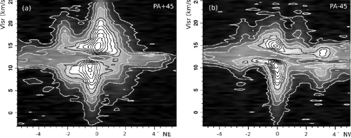
Figure 4: Position-velocity plots of the Rosette outflow ROF2, taken (a) parallel to the main outflow (at PA=+45 ^∘, along the flow axis) and (b) orthogonal to the flow (at PA=-45 ^∘, but offset SW by 1 arcmin to show the bright HV lobes). The x-axis is the offset in arcmin (positive offset in the left panel is NE along the main flow, in the right it is NW, orthogonal to the main flow); y-axis is the velocity (lsr). Lowest contours are 1 K, with a contour interval of 2 K (T_mb). Evidence of wings of HV emission, at velocities of $\pm 10kms^{-1}$, can be seen along both axes, out to separations of $\pm$ 2 arcmin from the central source.

One object in Table 1 (ROF2) is a well-known outflow source (AFGL961). Three others have published evidence of nearby shocked gas from emission line surveys in the optical [SII] or infrared (H₂) lines (Ybarra & Phelps, 2004; Phelps & Ybarra, 2005). The others are new flows. Notably there is a close correspondence between this list of outflows and the list of embedded young clusters found by Phelps & Lada (1997): the only CO outflow not associated with a nearby cluster (ROF5) lies outside their survey area (although inspection of the 2MASS K-band images around ROF5 showed no bright nearby cluster). Conversely, of the 7 embedded clusters identified by Phelps & Lada, only one (PL5) has no apparent associated outflow. Phelps & Lada also identified 10 IRAS sources in the region without an associated cluster; none of these have evidence of outflows in our survey. Moreover, by inspection of the datacube in position-velocity space, we find no evidence of HV gas in other regions around the Rosette Nebula (see Figure 1). In summary, massive high-velocity molecular outflows such as those listed in Table 1 are closely associated with young clusters containing luminous IRAS objects. IRAS objects without associated clusters do not show signs of HV outflows. In the following sections we discuss some of these flows, first individually, and then in the global context of the Rosette Nebula.

3.1.1 AFGL961

This was one of the first bright outflows to be discovered (eg Lada & Gautier, 1982), and published maps of the central region in ¹²CO lines indicated that the flow direction lies close to the plane of the sky (eg Schneider et al., 1998).

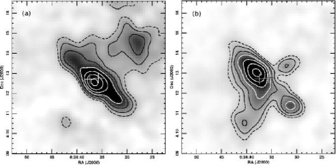
Figure 5: Contours and greyscale images of integrated blue and red-shifted gas in the region of the AFGL961 outflow (ROF2 in Table 1). Velocity ranges are: (a) -3 – +10 and (b) +15 – +25 $kms^{-1}$, respectively. The contours start at $4Kkms^{-1}(T_{mb})$ (2$\sigma$) and increment by factors of 1.5. The locations of the luminous infrared sources AFGL961 and AFGL961 II are shown by crosses (using 2MASS coordinates; AFGL961 is the eastern object).

Our new data (spectra in Fig. 2, and distribution of high-velocity gas in Figure 4a and 5) show that the CO outflow profile taken towards the infrared source extends over $\sim 30kms^{-1}$, and the main flow (at relative velocities up to $\pm 10kms^{-1}$) is well-collimated in the NE-SW direction, with a maximum extent of 5$\times$0.7 arcminutes (2.0$\times$0.3 pc). The ends of the red and blue-shifted lobes are abrupt, suggesting we are measuring the full spatial extent of the HV outflow. The peak emission in the highest-velocity blue and red-shifted gas is separated by $\sim$45 arcsec on either side of the bright IR source (AFGL961, the eastern of the two objects in Figure 5), indicating that this flow is inclined to the plane of the sky. However, this inclination is likely to be $<20\mbox{\,${}^{\circ}$}$, as the more extended red and blue-shifted lobes both show similar morphologies. Comparison with infrared images of H₂ v=1-0 S(1) emission from Aspin (1998) shows that the tip of the NE lobe is concident with the most distant clump of shocked H₂ (CA6), suggesting this is the bow shock at the end of the outflow jet.

Both the spectrum towards AFGL961 (Fig. 2) and position-velocity diagrams (Fig. 4) show a prominent and narrow self-absorption dip near the RMC systemic velocity. This dip appears spatially extended (over at least $\sim$4 arcmin in Fig. 4), implying it is due to absorption in a large cool cloud along the line-of-sight, rather than in a compact outer envelope around AFGL961 itself.

In addition to the NE-SW flow, the integrated CO maps (Fig. 5) show high-velocity gas in regions extending orthogonal to the main flow axis. It can be seen as HV emission extending to $\pm$3 arcmin in the position-velocity cut of Fig. 4b. If a separate flow, the origin appears to lie approximately 1 arcmin SW of AFGL961. This weaker flow appears to be bipolar, with blue and red-shifted gas dominating the NW and SE sides respectively, suggesting that the flow axis lies out of the plane of the sky. Infrared images of the region show shocked gas is also found in several other directions in addition to the dominant CO axis (Aspin, 1998). AFGL961 itself is known to contain several distinct components (eg Alvarez et al., 2004), and is associated with a young cluster (Poulton et al., 2008). Moreover, recent infrared images show the bright object 30 arcsec W of AFGL961 (known as AFGL961 II - see Fig. 5) has bipolar shocked H₂ emission extending at PA$\sim 345\mbox{\,${}^{\circ}$}$ (Li & Smith, 2005; Li et al., 2008). This may be associated with the second bipolar CO outflow.

In summary, the new extended high-resolution maps show that AFGL961 has a typical parsec-scale, well-collimated outflow, with evidence of a second orthogonal flow - possibly from AFGL961 II.

3.1.2 Outflow ROF1

Figure 6: Contours and greyscale images of integrated blue and red-shifted gas from the ROF1 outflow. Velocity ranges are: (a) 6 – 10 and (b) 15 – 23 $kms^{-1}$. Contours start from $2Kkms^{-1}$ and increment by factors of 1.5. The location of the luminous infrared source IRAS06329+0401 is shown by a cross.

The second region of clear spatially-extended HV wing emission is ROF1; this is closely associated with IRAS06329+0401 and cluster PL7 (see Phelps & Lada, 1997). The distribution of HV gas is shown in Figure 6. Both blue and red-shifted gas are found near the IRAS object, and there are also more distant regions of HV gas at projected separations of up to $\sim 1.6pc$. There is no embedded object near this separate HV gas in the Spitzer survey of Poulton et al. (2008), so it is unclear whether this is from a second fainter object or part of the flow from the bright IRAS source. The coordinates given in Table 1 are mid-way between the two regions.

3.1.3 Ensemble outflow characteristics

MacLow & Klessen (2004) and others have suggested that gas turbulence within a GMC has a strong effect on the efficiency of star formation. Moreover, it has been proposed that protostellar outflows, such as those described above, could provide a significant contribution to this turbulence. Consequently it is important to assess the global effects of all outflows within a GMC. The current dataset provides a census of HV outflows over a GMC of size $\sim 60$ pc, which is complete down to an outflow mass of $\sim 1M_{\odot}$. This potentially allows us to assess the global effect of such flows on the RMC. MacLow & Klessen note that, in most cases, the sizes of outflows are generally too small to be important within a GMC. The relatively compact nature of the outflows in the RMC confirms this. Even the largest - AFGL961 - is only 2pc across, or less than 5% of the size of the RMC. Within the individual young clusters, however, the outflows have a similar extent to that of the cluster itself, and their effect may be more significant. We can estimate the importance of the flows by comparing their kinetic energy, (${KE}_{of}$ in Table 1) with the turbulent kinetic energy of the associated large, dense molecular clumps (${KE}_{turb}$). Assuming the linewidth $dv(kms^{-1})$ is from turbulent broadening, then KE${}_{turb}(J)\sim 5\times 10^{35}M_{c}.dv^{2}$, where $M_{c}$ is the total clump mass in units of $M_{\odot}$; values of $KE_{turb}$ are listed in Table 1. Using published clump masses from the ¹³CO J=1-0 observations of W95, the outflow kinetic energy in Table 1 is 1-30% of the clump turbulent energy. After allowing for an underestimate of the outflowing mass by a factor of $\sim 3-10$ to account for inclinations and optical depths (eg Beuther et al., 2002 - see above), then the outflow kinetic energy is similar to the turbulent energy within the dense gas clumps. On a larger scale, however, the main part of the RMC has mass and velocity width of $7.5\times 10^{4}$ and $\sim 4kms^{-1}$ (W95), giving ${KE}_{turb}=10^{42}J$; this compares with the $1-3\times 10^{40}J$ from all the outflows (after including the correction factor described above). Therefore, although the outflows may be energetically significant on a stellar cluster scale, their effects are negligible on the tens of pc scale of the whole RMC.

3.2 Compact clumps and the inner edge of the cavity: global gas dynamics

The molecular gas in the vicinity of the Rosette Nebula shows a complex velocity structure, illustrated in the colour-coded image in Figure 7. Here, we show integrated emission from gas which is blue and red-shifted with respect to the RMC systemic velocity, and (in green) the emission from gas around the ambient cloud velocity. On the largest scale (tens of pc), the data shows a velocity gradient from NW-SE of $\sim 0.07kms^{-1}pc^{-1}$, similar to that noted by W95. The distant gas is distributed relatively smoothly, both spatially and in velocity. However, this gradient is clearly highly disrupted towards the central Rosette Nebula, where many compact clumps and clouds at different radial velocities are superposed along the line-of-sight. Some distinct features are apparent in the velocity-coded image which help in understanding the overall dynamics of the system. Examples are the NW ridge - a line of blue-shifted clumps seen most clearly $\sim 10$ pc NW of the centre (along the NW of the ellipse in Fig. 7), and the Monoceros Ridge - the abrupt edge of the SE molecular cloud $\sim 10$ pc SE of the centre (seen along the SE of the ellipse). These distinct features are described in the following sections.

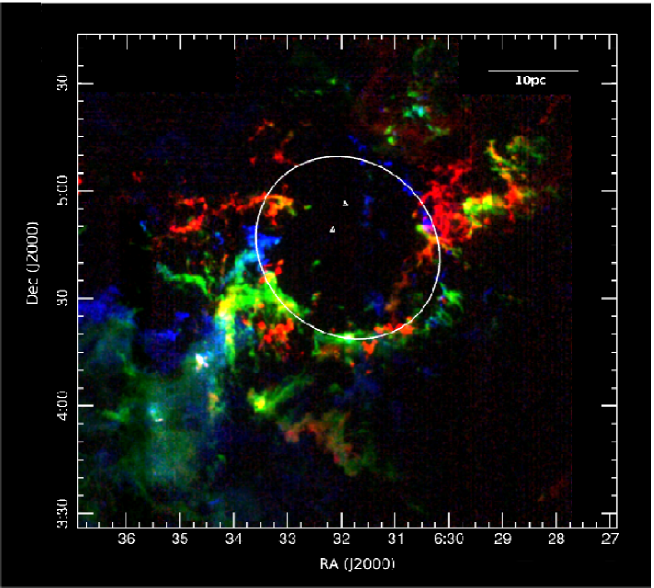
Figure 7: Colour-coded image of the molecular cloud around the Rosette Nebula, illustrating the global velocity structure. The blue, green and red colours represent integrated ¹²CO intensities in the velocity ranges (-2.8,+11.5), (+11.5,+16.6) and (+16.6,+25.1) $kms^{-1}$. The small triangles near the centre show the locations of the two most luminous O stars in the nebula (HD46223 and HD46150), and the ellipse shows a model of an inclined molecular ring, of radius $\sim 11$pc, and inclination 30^o to the line-of-sight (see text for details). The image is 61 pc (EW) $\times$ 56 pc (NS), assuming a distance of 1400pc.

The NW ridge is a line of compact blue-shifted clumps to the NW of the central O stars. These molecular clumps are all associated with dark absorbing globules and Elephant Trunks in the optical images (see section 3.3, Figure 9). Their high optical obscuration and blue-shifted profiles indicates they are on the nearside of the nebula, moving towards us (with respect to the systemic cloud velocity). Moreover there is a clear velocity gradient along the ridge; evidence of this can be seen in the colour-coded image in Figure 9. In order to help understand these data, we have fitted the positions, velocities and velocity gradients of the emission clumps using simple 3D Gaussians (see section 3.3.2). Using the centroid velocities of these fitted clumps, we investigate the velocity structure along the inner rim of molecular gas around the Rosette Nebula (to a projected radius of $\sim 15pc$ from the centre of the nebula, and a depth of 3.5pc (9 arcmin) from the inner edge of the rim). Figure 8 shows the velocity of these clumps as a function of $\phi$, the azimuthal angle around the rim. The velocity structure of much of the NW blue-shifted ridge (at $0\leq\phi\leq 120^{o}$) can be most easily fit with that of an expanding ring of radius 11pc, inclined at 30^o, with an expansion velocity of 30$kms^{-1}$ and a mean velocity of $16kms^{-1}$. This is illustrated by the ellipse in Figure 7. Evidence of gas clumps fitting such a ring can be seen in regions of $\phi$ up to 180 ^∘. Around the SE rim ($-180\leq\phi\leq-90^{o}$) there are few corresponding red-shifted clumps as predicted by the simple expanding ring model. Most emission here lies within $3kms^{-1}$ of the RMC systemic velocity, suggesting this material is not participating in the ring expansion. Nevertheless, the structure and velocity gradients across the SE cloud rim clearly indicate that this cloud is exposed to the O star radiation field; this suggests that expansion on this side may have been confined by the ambient cloud. The conditions of this cloud rim will be described further in section 3.3.2. Some additional blue-shifted emission is apparent on the E rim, at $\phi\sim-90^{o}$ in Figure 7 and 8, and this corresponds to an optically-dark obscuring cloud (eg Gahm et al., 2007). Notably, all of the dark clouds in the region of the Rosette Nebula - which are presumed to be in the foreground of the nebula - appear to be blue-shifted with respect to the cloud systemic velocity. This strongly suggests that all these foreground clouds are expanding away from the nebula towards us, and that most (but not all) of this expansion is in the form of a ring of material.

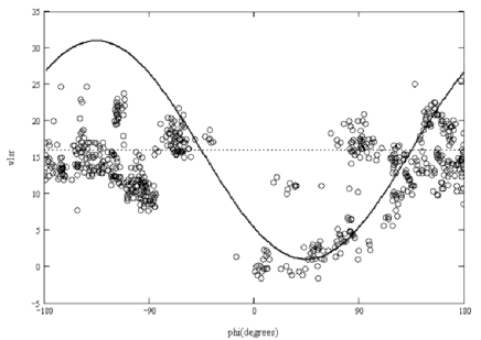
Figure 8: Radial velocity of CO clumps around inner rim of the Rosette Nebula plotted as a function of $\phi$, the position angle. The solid line illustrates the model of an inclined (i=30^o), expanding ($V_{exp}=30kms^{-1}$) ring of radius 11pc, with a mean velocity of $16kms^{-1}$ (given by the dotted line). See text for details.

Radio recombination lines show the ionised gas in the nebula has a mean velocity of 16.7$kms^{-1}$ (close to that of most of the CO emission - see Fig. 8) and a line fwhm of 30-40 $kms^{-1}$ (Celnik, 1985). This is consistent with the expansion velocity of the clumpy ring. Assuming a constant acceleration, then the expansion velocity and ring size implies a dynamical time of $\sim 0.8$ Myr, comparable with estimates of the system age of 2-3 Myr (Hensberge et al., 2000; Balog et al., 2007). The Rosette expanding ring has characteristics similar to the large molecular structure found around the nebula IC1396 (Patel et al., 1995). Here they have found a ring of clumpy gas with an expansion velocity of $5kms^{-1}$ and radius 12pc, surrounding an O6 star of age 2-3Myr.

3.3 Clumps in and around the Rosette Nebula

It has been known for many years that the Rosette Nebula is rich in dark obscuring material, first seen in optical images (eg Herbig, 1974). These structures range from extended dark globules and Elephant Trunks many arcminutes in extent (eg Gahm et al., 2006), down to “Teardrops” (eg Herbig, 1974) and “Globulettes” on scales of arcseconds or less (Gahm et al., 2007). Clearly, however, optical observations are limited to the dark absorbing regions in front of the diffuse nebular emission. Observations of the molecular gas, which have the advantage of tracing material thoughout the region, also show a highly clumped structure, albeit previously limited by observations to arcminute, or larger, scales (W95). Many of the largest optically-dark regions, however, have corresponding CO emission clumps (eg Schneps et al., 1980).

In the NW ridge, the present high-resolution data show that all of the blue-shifted CO clumps have associated obscuring optical regions, implying there is no blue-shifted gas lying behind the nebula: Figure 9 compares the distribution of blue-shifted gas (at velocities $v_{lsr}<4.7kms^{-1}$) with the optical H$\alpha$ image from the IPHAS survey (Drew et al., 2005). Conversely, none of the optically-dark clouds are associated with red-shifted gas, implying there is no foreground gas receding from us. An additional region of blue-shifted gas $\sim$20pc SE of the O stars can be seen in Figure 7. This also corresponds to obscuring foreground clumps (Patel, 1993), confirming that the dominant molecular gas motion in the RMC is expansion towards us, away from the nebular region.

Focussing on the NW ridge, in Figure 9 we have labelled some of the most prominent CO clumps facing the nebula, and in Table 2 we list their main parameters (clumps 1-15). Gahm et al. (2007) conducted optical studies of the highly compact globules in this region, and comparison with our new observations indicates that the present survey is able to detect CO emission from isolated globules with masses as small as $\sim 0.03-0.1M_{\odot}$. Examples of these are the three faint clumps 1 arcmin S of the cloud marked 6 in Figure 9, which correspond to Globules 47, 40 and 35 in Gahm et al. (2007). However, most clumps in the datacube lie in more complex and confused regions, which means the lower limit to their detectable mass is larger than this (see section 3.3.3). In the following sections, we discuss some of the salient features of the individual clumps.

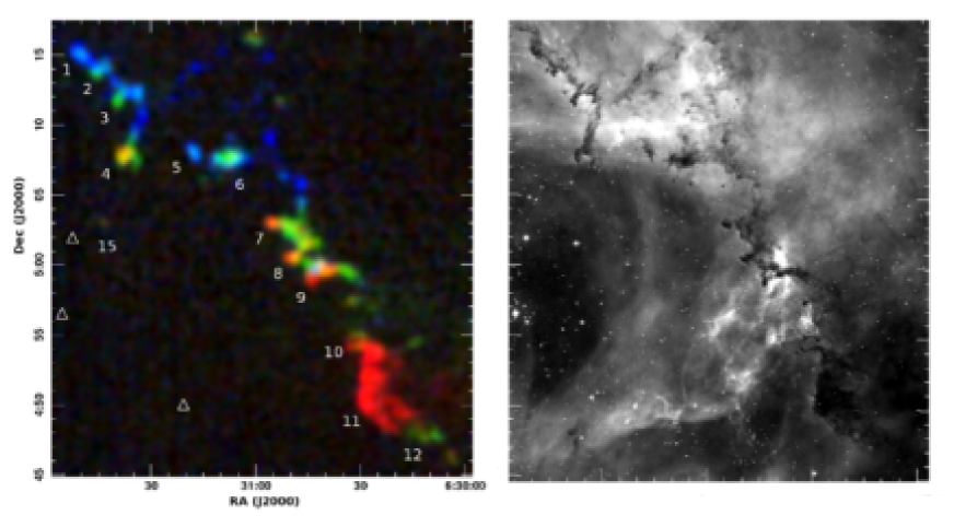
Figure 9: Colour-coded image of the blue-shifted CO emission in the NW ridge (left), compared with an optical H$\alpha$ image of the same region (image from the IPHAS survey, right). The exciting O stars of the nebula lie to the SW of these panels. The CO map is shows peak intensity, taken over 3 different velocity regions represented by different colours, where blue is $-2.8,-0.3kms^{-1}$, green is $-0.3,+2.2$ and red $+2.2,+4.7kms^{-1}$; this compares with the systemic cloud velocity of $+16kms^{-1}$. All of the molecular clumps can be identified with dark clouds in the optical image, implying all lie in front of the nebula. The main CO clumps are labelled, and their parameters are given in Table 2. All clumps, aside from #12 and 14, have a velocity gradient with increasing blue shift as a function of projected separation from the O stars (marked by the white triangles).

3.3.1 Clump parameters: dynamics and physical conditions

The colour-coded image in Figure 9 illustrates the detailed velocity structure of the NW clumps. Significant velocity shifts were known to exist across three of the brightest extended clumps in this region (Schneps et al., 1980; Gahm et al., 2006). The clearest example of a velocity gradient is seen in the “Wrench” trunk (marked as 4 in Figure 9). The resolution of the new dataset is sufficient to show that the majority of these NW clumps have radial velocity gradients of $\delta v/\delta r>1kms^{-1}pc^{-1}$; these are listed in the upper section of Table 2. In most of the well-defined NW clumps, the highest gradient occurs radially from the central O stars, in the sense that the blue-shift increases with increasing separation ($\delta v/\delta r<0$). For comparison with the NW clumps, the middle sections of Table 2 list parameters of several other distinct structures in the Rosette region, including bright inner clumps, bright regions of the sharp-edged rim at the interface between the nebula and RMC, and more distant and isolated clumps in the surrounding cloud. Finally, the lowest section in Table 2 lists parameters of centres of some of the smooth extended clouds seen in the datacube. These diffuse clouds were studied by Heyer et al. (2006) and are thought to be diffuse ambient molecular gas undisturbed by the activity of the O stars in the Rosette Nebula.

Table 2: CO line parameters of clumps and distinct objects in the vicinity of the Rosette Nebula.

Clump	RA	Dec	vlsr	$\delta$v/$\delta$r(a)	$\Delta$v(b)	$T_{mb}$3-2(c)	$T_{mb}$1-0	Ratio(d)	D(e)	Star	Notes
	(J2000)	(J2000)	($kms^{-1}$)	($kms^{-1}pc^{-1}$)	($kms^{-1}$)	(K)	(K)		(pc)	(f)
NW clumps
1	6 31 50.2	5 15 00	-0.6	-0.9	1.4	10.2	7.8	1.3	10.6	o
2	6 31 46.2	5 13 50	0.4	-2.2	1.9	8.0	8.9	0.9	10.2	o
3	6 31 39.4	5 11 47	0.8	-1.9	1.8	7.8	5.5	1.4	9.6	*
4	6 31 36.9	5 07 52	0.3	-3.7	2.0	11.8	9.8	1.2	8.2	*	Wrench clump(1)
5	6 31 18.0	5 07 55	-0.1	1.1	1.7	6.7	7.6	0.89	9.2	o
6	6 31 08.3	5 07 34	0.7	1.0	2.1	10.7	11.1	0.97	9.7	o	Clumps superimposed?
7	6 30 54.8	5 02 57	2.4	-2.0	1.3	10.2	8.9	1.2	9.4	-
8	6 30 49.5	5 00 26	2.5	-1.7	1.8	8.9	8.9	0.9	9.3	-
9	6 30 44.7	4 58 57	2.7	-1.6	1.4	6.6	7.1	0.92	9.5	-
10	6 30 32.8	4 57 24	1.9	-1.9	1.2	3.7	3.6	1.0	10.4	-
11	6 30 28.7	4 54 11	3.2	2.3	1.4	8.7	8.7	1.0	10.5	-
12	6 30 26.5	4 50 13	5.1	1.6	2.2	14.2	18.9	0.75	10.5	-	Unclear
13	6 30 11.1	4 47 42	1.4	-1.8	1.3	4.0	3.6	1.1	12.1	-
14	6 30 00.1	4 43 00	2.7	-0.9	2.0	5.1	3.6	1.4	13.5	-
15	6 31 43.7	5 03 06	2.2	0.2	2.4	1.7	1.2	1.5	6.1	*
Other inner clumps & rim
16	6 33 15.8	4 30 37	15.0	2.0	2.8	16.6	20.1	0.8	10.2	*	Monoc. Ridge(2)
17	6 32 29.1	4 39 57	14.2	1.6	1.6	10.2	11.6	0.89	4.4	o
18	6 33 14.1	4 46 17	10.3	-2.6	2.1	16.6	18.4	0.9	6.6	*	Extended Ridge(2)
19	6 30 30.7	4 49 27	15.9	2.1	1.6	21.1	22.4	0.94	10.1	-
20	6 32 39.2	4 55 19	15.6	2.7	1.7	9.8	10.9	0.9	3.7	o
21	6 32 29.3	4 30 32	15.9	-2.4	1.1	10.7	6.7	1.6	8.0	o
22	6 32 39.4	4 26 37	13.0	2.4	1.5	12.6	10.7	1.2	9.8	o	SSW rim
23	6 31 07.6	4 27 37	16.5	0.7	0.8	16.2	23.3	0.69	11.0	*
24	6 33 10.7	4 37 37	20.6	0.9	1.9	20.3	16.7	1.2	7.8	o
25	6 32 01.0	4 27 28	13.7	0.7	1.5	6.2	5.6	1.1	9.1	o
26	6 32 59.5	4 30 15	14.3	2.8	1.4	14.0	13.3	1.0	9.4	*	Monoc. Ridge(2)
27	6 31 02.8	4 20 27	13.1	0.2	1.4	8.7	10.0	0.87	13.7	-	S rim
28	6 31 25.2	4 19 08	14.4	0.7	1.0	17.1	14.7	1.2	13.2	o	S rim
29	6 33 08.4	4 47 01	10.9	-1.3	1.5	7.6	6.7	1.1	6.0	*	Pillar(3)
30	6 31 51.2	4 23 13	15.5	-0.5	1.1	6.6	6.0	1.1	10.9	o
31	6 32 59.2	4 23 44	17.2	2.7	1.9	10.7	9.8	1.1	11.6	*
32	6 33 22.6	4 40 44	10.4	1.4	1.6	13.3	8.4	1.6	8.2	*	Monoc. Ridge(2)
33	6 31 20.6	4 22 55	14.9	-2.3	1.5	5.8	6.2	0.94	12.0	*	S rim
34	6 33 08.0	4 40 13	17.0	1.5	2.7	10.2	10.2	1.0	7.0	o
Distant clumps
35	6 32 08.9	4 05 15	14.2	-0.2	0.7	8.7	10.7	0.82	18.1	o
36	6 33 21.5	4 19 05	18.2	1.7	2.0	11.8	10.7	1.1	14.4	o
37	6 34 18.6	4 47 42	11.2	-0.8	1.6	15.8	15.6	1.0	13.0	o
38	6 34 14.1	3 45 40	12.7	-0.5	0.9	12.2	12.9	0.95	28.9	o
39	6 30 36.9	5 23 55	12.8	1.3	1.4	18.7	22.0	0.85	16.6	-
40	6 28 32.2	4 58 58	15.8	-0.6	1.3	12.7	15.6	0.82	22.5	-
41	6 29 55.5	4 31 16	14.4	1.1	2.0	19.1	18.2	1.0	15.6	-
42	6 34 24.0	3 48 41	14.7	-0.1	0.5	8.2	8.9	0.92	28.3	o
43	6 30 34.0	4 10 07	14.2	-0.4	0.9	4.6	4.7	0.97	18.9	-
44	6 35 02.0	4 25 19	8.2	-1.7	1.1	12.9	14.4	0.89	20.2	*	IRAS source(4,5)
45	6 33 54.9	4 04 50	10.1	0.6	0.5	2.6	3.1	0.83	21.1	o
46	6 34 01.2	4 02 23	9.6	-0.3	0.8	4.2	3.9	1.1	22.3	o
47	6 35 01.0	4 21 17	13.7	-1.7	0.8	7.6	9.1	0.84	20.8	*
48	6 32 06.4	4 15 10	16.7	-0.6	0.7	12.2	14.7	0.83	14.0	*
49	6 31 48.2	4 11 34	17.3	0.8	0.9	10.5	7.8	1.4	15.6	o
Extended smooth clouds
50	6 35 46.0	3 39 10	11.1	-0.4	1.6	4.2	4.9	0.86	36.1	o
51	6 30 10.0	5 19 00	17.8	0.5	1.0	2.9	7.1	0.41	17.1	-
52	6 31 55.7	3 44 09	16.2	-0.4	1.3	7.4	10.2	0.73	26.7	o
53	6 32 47.5	5 36 56	15.9	-0.5	0.4	4.0	6.8	0.59	19.7	-
54	6 36 31.8	4 27 04	5.1	0.1	1.4	2.7	5.5	0.5	28.0	o
55	6 28 10.2	5 00 46	19.8	0.1	0.9	2.0	5.6	0.36	24.4	o
56	6 34 01.8	5 18 10	10.8	0.3	0.5	4.6	6.0	0.76	16.2	-
57	6 25 57.6	4 09 50	14.8	0.3	1.1	5.3	8.7	0.61	28.1	-

Notes to Table 2: (a) Velocity gradient over 60–100 arcsec distance around given coordinate, measured radially from most luminous O star (HD467223); (b) Velocity width (fwhm) of J=3-2 ¹²CO line from full spatial resolution map, after deconvolution with instrumental velocity resolution ($0.45kms^{-1}$); (c) Main beam brightness temperature of ¹²CO J=3-2 line, after smoothing to same spatial resolution as J=1-0 data (45 arcsec); (d) Ratio of $T_{mb}$; (e) Projected separation from HD46223; (f) An asterix indicates a star or compact infrared source (from Spitzer 8$\mu m$ and/or 24$\mu m$ images) can be identified with the molecular clump, ’o’ indicates no star, ’-’ indicates region not covered by Spitzer images. References: (1) Gahm et al. (2006); (2) Schneider et al. (1998); (3) Balog et al. (2007); (4) Patel et al. (1993); (5) White et al. (1997)

On the SE side of the central cavity, most of the clumps also have significant velocity gradients, and most have $\delta v/\delta r>0$. Optical images show that these molecular clumps do not have clear corresponding dark clouds, and therefore lie towards the far side of the nebula. This gas appears to be accelerating away from us on the far side. There is one notable exception to this: the red-shifted clump 8 pc SE of the central star (Clump 21, see Fig. 7), which appears to be accelerating in the opposite direction. Inspection of the optical image shows this actually corresponds with a dark obscuring cloud, so it lies in front of the nebula and is an isolated clump undergoing acceleration towards us.

Assuming the velocity gradients are due to radial motion away from the central O stars, then the radial clump acceleration is given by:

$$a_{c}=0.5[(v_{c}.{\delta~{}\!v}+{\delta~{}\!v}^{2})/{\delta~{}\!r}]$$

Here $v_{c}$ is the clump velocity relative to the molecular cloud systemic velocity and $\delta~{}\!v$ the velocity difference along the cloud of length $\delta~{}\!r$. The apparent clump acceleration, $a^{\prime}$, depends on the inclination of the accelerating surface to the plane of the sky: $a^{\prime}=a_{c}/({sin}^{2}~{}\!i.cos~{}i)$. In Figure 10 we show the radial acceleration of the clumps in Table 2 assuming $i=30\mbox{\,${}^{\circ}$}$ (equal to that of the expanding ring in section 3.2), plotted as a function of projected distance from the centre of the nebula. The RMC systemic velocity of $16kms^{-1}$ was used to determine $v_{c}$. The plot shows a general decrease with increasing separation, suggesting that clump acceleration is caused by the stars in the centre of the nebula. However, some clumps have relatively low apparent velocity gradients; these may be moving closer to the plane of the sky than the inclined ring.

Observations of molecular gas clumps and globules near other nebulae show velocity gradients of a few $kms^{-1}pc^{-1}$, similar to those in Table 2 (eg Lefloch & Lazareff, 1995; Gonzalez-Alfonso et al., 1995; Pound, 1998; Bachiller et al., 2002). One model for the acceleration of molecular gas in such clumps is through a rocket effect, whereby the clumps are gradually photoevaporated by the O-star photons, and the pressure from the photoionised wind from the ablating surface drives the clump away from the star (eg Oort & Spitzer, 1965; Bertoldi & McKee, 1990). Bertoldi & McKee (1990) have developed this Radiatively-Driven Implosion (RDI) model and derive (in their eqn. 4.2), the resulting mass loss rate of clumps of radius $R_{c,p}(pc)$ and mean density $n_{H_{2}}(cm^{-3})$. From the mass loss rate, we can estimate the resulting clump acceleration:

$$a=5.6\times 10^{-6}.\phi.cos~{}{i}.S_{{}_{50}}^{0.5}.D_{p}^{-1}.R_{c,p}^{-1.5}.V_{r,_{10}}.n_{H_{2}}^{-1}\ \ [{m}{s}^{-2}]$$

where $D_{p}$ is the projected separation from the O star (in pc), $S_{{}_{50}}$ the ionising flux from the star(s) in units of $10^{50}s^{-1}$ (equal to the estimated total ionising flux from the Rosette O stars), and $i$ is the projection angle of the clump from the plane of the sky. The Rocket velocity of the ionised particles is $V_{r,_{10}}$ (in units of $10kms^{-1}$ - typical for most models), and $\phi$ is a dimensionless factor governing the clump mass loss rate, taken to be $\sim 3.0$ for the conditions in the Rosette Nebula (see Bertoldi & McKee, Fig. 11). The solid line in Figure 10 shows the predicted clump acceleration as a function of distance from the O stars, for clumps of radius 0.1 pc (30 arcsec diameter) and density $3\times 10^{4}cm^{-3}$ (giving a clump mass of 8$M_{\odot}$ - similar to that of the Wrench Clump measured by Gahm et al., 2006). The model fits the upper envelope of the data points, using an inclination of $30\mbox{\,${}^{\circ}$}$; the Wrench clump and other NW clumps have the highest acceleration in the plot and fall near the model line. In general, however, most clumps lie below the model prediction, suggesting they have a lower inclination (lying closer to the plane of the sky), or that the acceleration efficiency of distant clumps is lower than predicted.

Also shown in Figure 10 is the estimated lifetime to photoevaporation. For clumps within 5pc of the O stars, this is very short - less than 10% of the age of the Rosette Nebula. Even the distant clumps have relatively short lifespans compared with the nebula age of $\sim 2Myr$, implying they are transient phenomena.

Figure 10: Derived acceleration (in ${m}{s}^{-2}$) of clumps in the Rosette Nebula plotted against projected distance from the nebula centre (assumed to lie at $06^{h}32^{m}10.2^{s}+~{}04^{o}49^{\prime}28^{\prime\prime}$, the location of the most luminous star HD46223). The solid line shows a model of acceleration by photoevaporation by the central O stars based on Bertoldi & McKee (1990). The datapoints have been corrected for inclination assuming $i=30\mbox{\,${}^{\circ}$}$ (see text). The symbols represent the NW clumps (squares), other central clumps (triangles), and more distant compact clumps (stars). The crosses illustrate the velocity gradients and apparent acceleration in the smooth background clouds, thought to be unaffected by the O stars.

As well as the acceleration, the internal velocity dispersion ($\Delta v$) is higher in the innermost clumps. For clumps with $D_{p}\leq$13pc, $\Delta v=1.6\pm 0.44kms^{-1}$, marginally larger than the distant clumps ($1.2\pm 0.46kms^{-1}$). It is not due to smearing of the velocity gradient due to the finite beam size, which in all cases would be less than $0.3kms^{-1}$. This suggests that the turbulence in the clumps is affected by the interaction and acceleration of the O-star winds. Line emission from the extended smooth clouds is narrower, with widths of $1.0\pm 0.4kms^{-1}$.

We can estimate the clump physical conditions by examining the ¹²CO 3-2/1-0 line ratios. However, the results of such analysis are subject to limitations and uncertainties: the optical depths in these lines can be large, the effects of PDRs can change the line excitation, and the lines may be tracing gas at different depths in the clumps (with different kinetic temperatures, and/or resulting in different beam filling factors). Molecular line ratios have been investigated in several similar regions, including detailed studies of individual clumps within the RMC (eg Patel et al., 1993; Gonzalez-Alfonso & Cernicharo, 1994; W95; White et al., 1997). PDR models have also been applied to a few individual lines of sight in the RMC on a 2 arcmin scale (see Schneider et al., 1998). Although data from many transitions and isotopomers are needed to uniquely interpret the results, the large scale and dynamic range of the present data does allow us to investigate general trends in the clumps across the whole of the GMC.

Using the J=1-0 ¹²CO data from Heyer et al. (2006), we include in Table 2 the 3-2/1-0 line ratio of clumps and the clouds in the region, after convolving the J=3-2 data to the same resolution (45 arcsec). Note that the objects chosen for this analysis are distinct isolated features in the clouds, and are well separated from the HV outflows. The clumps have ratios ranging from 0.4-1.8, and in Figure 11, we plot the line ratio against the separation from the brightest O star HD46223 (roughly the luminosity centre of the nebula). In general, this shows a decrease in ratio as a function of separation. The distant, extended smooth clouds (shown by crosses) have ratios significantly lower than the clumps.

Figure 11: Ratio of J=3-2 / 1-0 ¹²CO for clumps in the Rosette Nebula, plotted against the projected separation from the nebula and luminosity centre. The symbols represent the NW clumps (squares), other central clumps (triangles), more distant compact clumps (stars), and the centres of the extended distant clouds (crosses). The curves show the predicted line ratios using the radiative transfer model “Radex” for three different gas densities: $3\times 10^{3}$ (dashed), $3\times 10^{4}$ (solid) and $3\times 10^{5}cm^{-3}$ (dot-dashed). We use a constant CO column density of $10^{17}cm^{-2}$ and linewidth of $1.5kms^{-1}$, and assume the gas and dust temperatures are equal. Kinetic temperature is derived from the separation from the luminous star (see text for details).

Using the program ”Radex” (van der Tak et al., 2007) we can derive 3-2/1-0 line ratios for different gas densities and temperatures, assuming an isothermal gas. With a CO column density $N_{L}(CO)=10^{17}cm^{-2}$ and a linewidth of $1.5kms^{-1}$, this gives the line ratio diagram in Figure 12. This column density is equivalent to an extinction, $A_{V}=1.0$, assuming a CO abundance of $10^{-4}$ and $N_{L}(H_{2})/A_{V}=10^{21}cm^{2}/magn$. $A_{V}=1.0$ is considered a lower limit for most of the clumps. In particular, studies of two of the NW clumps show $A_{V}\sim 1-10$ (Gonzalez-Alfonso & Cernicharo, 1994; Patel et al., 1993). CO column densities higher than $\sim 3\times 10^{17}cm^{-2}$ ($A_{V}=3$) will result in high optical depths in both the 1-0 and 3-2 lines, and ¹²CO line ratios close to unity. That the observed 3-2/1-0 ratios in most clumps are higher than this suggests that most line emission is from warm gas near the clump surface, at around $A_{V}\sim 1$, and without extreme line optical depths. This suggests that the clumps are being heated externally and CO is tracing the heated outer layer, similar to the model for CO emission from cores near the Orion cluster (Li et al., 2003).

Figure 12: Plot of J=3-2 / 1-0 ¹²CO line ratio as a function of gas kinetic temperature and total volume density, using the “Radex” code (van der Tak et al., 2007). This uses a linewidth of $1.5kms^{-1}$ and CO column density of $10^{17}cm^{-2}$. For comparison, most of the observed clumps have ratios of 0.5-1.6.

To compare the observed line ratio with the model, we include in Figure 11 three curves showing the predicted 3-2/1-0 ratio as a function of separation from the centre of the nebula, assuming equal gas and dust temperatures and dust heating by the central O stars. The luminosity centre of the nebula is assumed to be at the location of the O4.9V star HD46223. In the interest of simplicity, we assume that all clumps have similar mean volume densities in the emitting region, and ignore projection effects. We adopt a simple power law for dust kinetic temperature in the clumps:

$$T=35~{}K.[L/{10^{6}L_{\odot}}]^{1/6}.[a/{0.1\mu m)}]^{-1/6}.[R/{10pc}]^{-1/3}$$

This assumes heating by central O stars of total luminosity $L=10^{6}L_{\odot}$ at a mean location of the brightest star (HD46223), and a grain emissivity based on Mie theory with a grain size $a=0.1\mu m$ (eg Krügel, 2003). The predicted line ratio is plotted as a function of $R$ for three values of the gas density, $n_{H_{2}}$. The datapoints are consistent with typical gas densities of $3\times 10^{4}cm^{-3}$ (shown by the solid line). This value is sufficiently high that gas and dust will be closely coupled (eg Galli et al., 2002), resulting in similar gas and dust temperatures. Gas in the smooth distant clouds (shown as crosses) lies below this line, and likely has a lower density, or lies at a larger de-projected distance and is cooler than predicted.

In summary, the plot shows that line ratios and derived clump temperatures are consistent with radiative heating by the central stars. As noted above, it is likely this is the clump surface temperature; internal clump temperatures are not accessible to the ¹²CO lines because of high optical depths, and their determination would require measurements using less abundant isotopologues.

3.3.2 The SE and S rims

The sharply-delineated SE rim, known as the Monoceros Ridge, is a clear example of the interface between O star radiation field and a Molecular Cloud (Blitz & Thaddeus, 1980; Schneider et al., 1998). As noted by Schneider et al., the region shows a sharp drop in molecular emission on the side of the cloud facing the O stars. They also noted that it is composed of several discrete components in position-velocity space. In Figure 13 we show a colour-coded image of the J=3-2 line in this region, as well as the edge of the cloud to the S of the central cavity (the S rim). Along both SE and S rims, the molecular cloud has a sharply-defined bright edge, spatially unresolved on one side. This indicates that the edge facing the O stars is $<$15 arcsec (or 0.1pc) across, ie it is likely to be a thin structure viewed almost edge-on. In the lower-resolution J=1-0 images (Heyer et al., 2006), the limb-brightening is less clear, and the J=3-2/1-0 line ratio (after convolving the 3-2 data to the same resolution) shows a peak at the bright edge of 1.1, dropping gradually into the molecular cloud to $\sim 0.8$. This suggests that the limb brightening of the J=3-2 line is due to a temperature peak at the cloud edge of 30K (averaged over a 45 arcsec beam), dropping to $\sim$20K in the cloud core (cf Figure 12).

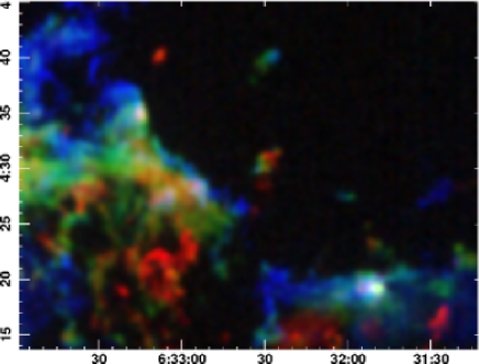
Figure 13: Three-colour image of J=3-2 ¹²CO integrated intensity in the vicinity of the SE and S rims, illustrating the velocity structure at the interface between the molecular cloud and the central cavity. The blue, green and red colours represent integrated intensities in the velocity ranges 11.5-13.7, 13.7-15.8 and 15.8-17.9 $kms^{-1}$ respectively. Resolution of this image is 20 arcsec, and the exciting O stars lie to the NW of the map. The two bright broad-lined objects in the S and SE rims are associated with the outflows ROF4 and ROF7 and with IRAS objects.

In addition to the sharp-edged structure, the SE-S cloud rims show a velocity gradient, with $\delta v/\delta r\sim 2-3kms^{-1}pc^{-1}$. This is mostly orthogonal to the edge, and can be seen in the colour-coded image in Fig. 13, where the rim facing the O stars is blue-shifted, and the emission becomes more red-shifted deeper into the RMC. The gradient is of similar magnitude but opposite sign to that seen across the NW clumps (Table 2), suggesting that the rims lie on the far side of the nebula, and that gas is being accelerating away from us. This relative location along the line-of-sight is confirmed by the absence of corresponding dark absorbing clouds in optical images, and contrasts with the NW side, where every blue-shifted CO clump has a clear corresponding dark cloud (cf Figure 9). The bulk molecular gas velocity of the SE rim gas is $+15kms^{-1}$, similar to that of the nebula and RMC itself. Note that this is the projected velocity; the true velocity may be higher if acceleration has occurred mostly in the plane of the sky (for example, if it is being viewed edge-on).

In addition to a velocity shift, the datacube also shows an increase in linewidth across the SE rim, from $1.2kms^{-1}$ at the blue-shifted edge, to $2.4kms^{-1}$ towards the molecular cloud core. Although in some regions this broadening may be due to multiple clumps at different velocities along the line of sight (eg Schneider et al., 1998), the general trend throughout the rims is that the clump gas velocities are more dispersed further into the cloud.

Both the SE-S molecular rims and the NW ridge (see above) are at a similar separation from the O stars, and are presumably experiencing a similar photoionisation flux. Other physical characteristics (CO linewidth, velocity gradient, temperature) are similar in both the SE-S molecular rims, and the NW clumps. However these regions clearly have different morphologies, with small filling-factor clumps elongated in the radial direction in the NW (Fig. 9), and a large filling-factor molecular rim orientated tangentially in the SE-S (Fig. 13). The reason for this difference is likely due to the different molecular gas densities in these two directions. As the gas in the RMC to the SE disperses, the contiguous rim is likely to evolve into a series of more dispersed isolated clumps, similar to that currently found in the NW.

3.3.3 Clump mass distribution

The images of CO and optical emission (Figures 1, 7 & 9) show that much of the gas within 25 pc of the Rosette Nebula appears highly clumped over a wide range of size scales; several authors have also noted that the RMC contains a large number of compact, low-mass clumps. Molecular observations of the bright SE section of the RMC have been used to estimate the clump mass distribution in this region (W95, Schneider et al., 1998). However, the large area coverage and simultaneous high spatial resolution of the present dataset potentially allows us to measure the clump mass distribution over a relatively large dynamic range, and to search for differences in the clump mass distribution over the cloud. To identify individual clumps, we have employed the Starlink CUPID package (Berry et al., 2007), with the 3-D Gaussian fitting algorithm, based on Stutzki & Güsten (1990). This allows a direct comparison with similar analysis of other GMCs (eg Kramer et al., 1998, and refs. therein). To minimise the ambiguity of clump identification and increase the robustness of the results, we set rather conservative lower limits to the peak brightness temperature (5.5K, $T_{mb}$), clump size (20 arcsec), and linewidth ($0.7kms^{-1}$). This technique identified 2050 clumps with these limits over the complete area shown in Fig. 1.

Reconstructing a model datacube with the identified clumps generates $\sim 70\%$ of the compact emission flux ($<2$ arcmin across). However, very little of the large-scale emission ($>5$ arcmin) from the extended smooth clouds is picked up using this technique, and only 2$\%$ of the identified clumps have sizes larger than 5 beamwidths, as the Gaussian clump-fitting method tends to subdivide larger clumps. Although it is likely that the ¹²CO transition is optically thick - particularly in the dense cores, we assume here that the integrated intensity scales linearly with the mass (eg W95), and use published ¹³CO studies of individual clumps (where the masses can be measured more accurately) to scale the results. In particular, Patel et al. (1993) have estimated the mass of Globule 1 (listed as Clump 44 in Table 2), and Schneps et al. (1980) and Gahm et al. (2006) measured the “Wrench clump” (Clump 4 in Table 2). Other isolated bright regions have also been observed in ¹³CO in W95. For those clumps with published masses, our integrated J=3-2 ¹²CO intensity and the published masses scale linearly within a factor of 2 over the mass range 5-1000$M_{\odot}$. By adopting this scaling, we derive the clump mass distribution for the whole mapped region shown in the upper histogram of Figure 14. This can be fit by a slope of -0.8 (shown by the dashed line) for masses in the range 3-100$M_{\odot}$. Although clumps (or “Globulettes”) with masses as small as $\sim 0.1M_{\odot}$ can be detected in some sparse regions of the present datacube (see Fig. 9), the confusion limit is considerably higher in most regions, which results in the drop in the number counts below $\sim 3M_{\odot}$ in Fig. 14.

The fitted slope in Fig. 14 implies a mass power law, $dN/dM\sim-1.8$, over the range 3-100$M_{\odot}$, for the whole RMC. This compares with -1.6 found by Schneider et al (1998) using two different datasets covering the SE region alone, and -1.3 measured by W95 for the SE region using a different clump-finding algorithm (although their technique was noted by Kramer et al. to blend low-mass Gaussian clumps, resulting in a flatter slope). This value is similar to that found for other large-scale molecular clouds (eg Kramer et al., 1998; Heyer et al., 2001), suggesting there is no excess of compact, low-mass clumps in the Rosette Nebula, and that it is a typical GMC. There is marginal evidence of a steeper power law at the high mass end (above 100$M_{\odot}$), although this would need confirmation using a less abundant and hence optically thinner molecular species.

Figure 14 compares the mass distribution for clumps in the complete datacube (within a projected separation of $\sim 25$ pc from the O stars), clumps in the inner region of the Rosette nebula (separation $<14$ pc), and clumps in the innermost expanding ring (section 3.2). CO images (eg Fig. 9) show that these inner regions are apparently highly-clumped, and are presumably more disrupted by the central O stars (see section 3.3.1 above). However, the three histograms show that not only is the power spectrum similar to that of other GMCs, but there is no clear difference in the mass distribution of clumps close to the O stars compared with that of the RMC as a whole.

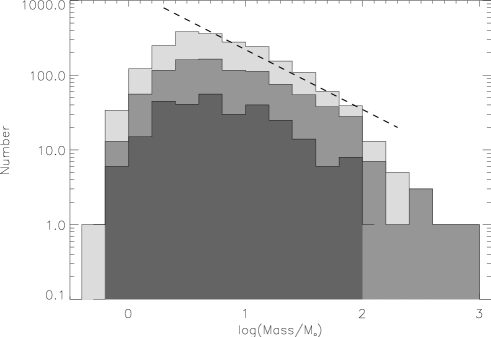
Figure 14: Histograms of clump integrated intensity in the Rosette region. The upper faint grey plot includes clumps found over the whole map area, the middle includes those for the inner region (within 14pc of the centre), and the lower darkest grey plot includes only the clumps in the expanding ring noted in section 3.2. Masses are estimated by scaling from a published multi-isotopomeric study of one of the clumps (Patel et al., 1993). The dashed line represents a mass distribution $N(M)\propto M^{-0.8}$.

3.3.4 Association of molecular gas and young stars

Seven of the 14 IRAS far-infrared objects in the Rosette region were shown by W95 to be associated with bright molecular gas clumps, and were presumed to be young embedded luminous stars. The present CO study shows that 7 luminous IRAS objects in the RMC also have associated high-velocity outflowing gas (see Table 1), 6 of which are common to the list of clumps in W95.

More recent infrared surveys have shown that several of these IRAS objects may actually be composed of young stellar clusters rather than individual luminous stars (eg Phelps & Lada, 1997; Poulton et al., 2008). Moreover, as noted in section 3.3.2 above, the CO clumps identified in W95 decompose into many sub-clumps at increased spatial resolution. Poulton et al. (2008) and Balog et al. (2007) conducted a detailed 3 – 70$\mu m$ continuum study of a significant fraction of the Rosette region with the Spitzer telescope. By comparing their data with our CO maps, we can examine the association between the young infrared objects and the molecular gas at increased resolution and towards lower luminosity stars. This is best done at 24$\mu m$, where the resolution is high enough to identify individual stars, and the youngest, most embedded objects can be seen.

Figure 15 shows a superposition of the infrared-excess stars identified by Poulton et al. on the J=3-2 CO peak intensity. The crosses show stars with SEDs fitted by Poulton et al. using a circumstellar disk model (which we loosely term SED Class II); the squares represent those which require an additional envelope to fit the excess (here called Class I). Many (but not all) of the Class I (envelope) objects are associated with clumps of molecular gas. There are also clearly some regions – such as that around the main cluster NGC2244 itself, in the NW of this image - which contain many Class II (disk) objects, but which are devoid of CO. Conversely, there are regions with apparently bright and clumpy molecular gas but which have very few Class I or II stars; examples are the clumps 15-40 arcmin SSE of the main cluster. Both Poulton et al. and Balog et al. noted the dearth of Class I but abundance of Class II objects within the cluster NGC2244. Can these different sets of observations be reconciled?

CO emission from a disk-only (Class II) source would not be detected with the present observations: for a typical disk of 300 AU radius, an optically thick line and a mean temperature of 40K, beam dilution would give $T_{mb}\sim 0.04K$, an order of magnitude below the current observational limit. However, envelopes around young stars typically have radii an order of magnitude larger, and therefore would be detectable in our data. Looking at their individual Class I objects, 30/36 in the mapped area have nearby CO emission (within 30 arcsec). However, this is formally an upper limit to the association of gas and young stars, as in some cases the CO may just lie along the line-of sight to the star.

Using the same $I_{CO}$:$M_{clump}$ scaling factor as measured above (see section 3.3.3), we can estimate gas mass limits around the 6 Class I objects identified by Poulton et al. using complete SEDs, which have no associated CO. The resultant upper limits for their clump masses are $\leq 0.2M_{\odot}$. However, it may be that these objects are misclassified, and are actually Class II disks viewed edge-on; a highly-inclined disk can mimic the SED of envelope-dominated structure due to the high extinction to the central star. In this case, we would not expect to detect CO. The relatively small number of Class I objects without associated CO (6, compared with 750 Class II objects) is consistent with this intepretation, as long as the disks are geometrically thin.

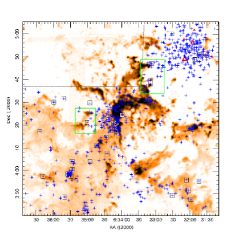
Figure 15: Map of peak J=3-2 ${}^{12}CO$ emission, with the IR-excess stars identified by Poulton et al. (2008) superimposed. The dashed line towards the upper left marks the boundary of the area studied in the infrared. The blue crosses represent stars with an infrared excess, where the SED can be fit by a disk, and those shown by squares require an addition envelope component. The large red triangles represent the O stars illuminating the Rosette Nebula. The two green rectangles are the areas illustrated in more detail in the middle and right panels of Figure 16.

Poulton et al. required detections at multiple wavelengths to classify the objects. However, several additional compact objects can be seen in their longer-wavelength data, which were not formally identified as YSOs, either due to incomplete sky coverage at all wavelengths or because they were too faint at some wavelengths. Examples can be seen in the NW ridge, where compact 24-${\mu}m$ objects are associated with the tips of the 2 or 3 of the CO clumps (see Fig. 16, left panel). Optical images of the tip of the Wrench Clump also show evidence of an embedded star or compact reflection nebula (Gahm et al., 2006). Many of the associations of YSOs with CO clumps are found near the bright rims at the edges of the molecular clouds, and resemble the young stars found in some evaporating globules within the Eagle Nebula (eg McCaughrean & Andersen, 2002). Figure 16 shows in detail some of the clearer examples of CO clumps (given by the contours) and their association with 24$\mu m$ point sources and bright-rimmed clouds. As argued above, these peaks in the CO emission are too bright to be arise from a compact disk, and are likely to be evaporating envelope gas. This is confirmed by their IR classification as envelope-dominated in several cases (see Poulton et al.).

If the $24\mu$m compact sources in the NW globules are also confirmed as young stars, it is likely they will have a similar velocity as that of the CO gas – typically, the relative velocity of stars and their gas envelope is $<1kms^{-1}$ (Covey et al., 2006). This would imply that the NW ridge is forming stars which have a relative velocity of $15kms^{-1}$ compared with the rest of the RMC. This compares with the escape velocity of the RMC of $\sim 6kms^{-1}$, implying this will eventually eject a ring of young stars.

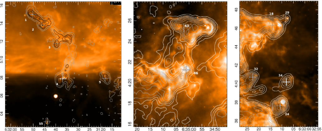
Figure 16: Superposition of the Spitzer $24\mu m$ image on the peak J=3-2 CO emission (contours) in some of the regions with Class I and II stars identified by Poulton et al (2008) or where 24$\mu m$ point-like sources can be identified, and which have associated clumps in the CO datacube. The crosses show some of the CO clumps and their identifications in the list in Table 2. CO contours start at 2.7K, with intervals of 2.7K ($T_{mb}$). Axes are RA/Dec (J2000).

4 Discussion - the effects of the OB stars on the molecular cloud

The molecular clouds in the vicinity of the Rosette Nebula, as revealed in the new CO images, show a highly clumpy morphology, with sharp-edged clouds mostly facing the OB stars. The overall clumpy structure is very similar to the simulated images from SPH modelling of the effects of O-star photoionisation on a turbulent molecular cloud (cf Dale et al., 2007, Fig. 2). Their models suggested that the effect of the luminous stars on the surrounding star formation rate is rather modest; triggered star formation in such circumstances is not a very significant phenomenon.

The results of the present large-scale mapping of the molecular gas shows a good correlation between luminous young clusters (with luminosity $\geq 10^{3}L_{\odot}$), high velocity outflows and bright regions of molecular emission. Moreover in several cases, individual stars with envelopes are also associated with bright CO clumps. In most cases, these are at the edges or rims of the GMC, facing the central nebula. A particularly clear example is Clump 44 in Table 2, seen near the top of the middle panel in Figure 16. Here a point-like 24-$\mu m$ source lies at the centre of the head of the CO clump. Patel et al. (1993) identified an IRAS object near this location, with a luminosity of $\sim 100L_{\odot}$ (although this may be an upper limit as the $100\mu m$ flux is confused). Patel et al. and White et al. (1997) noted that there was a significant velocity gradient along the length of this globule.

The new data (Figure 17) shows that this velocity gradient is remarkably constant, at $1.7kms^{-1}pc^{-1}$ over a distance of 1.7pc (270 arcsec) behind the star. It is unclear at present whether the RDI model (eg Bertoldi & McKee, 1990; Lefloch & Lazareff, 1994) can predict such an extended and constant acceleration in the molecular gas behind such clumps; in general most of their results show curvature in the position-velocity diagrams. Furthermore the RDI model predicts significant velocity gradients only in the relatively short-lived (and hence rare) “pre-cometary phase”. The present results (see Table 2) show that significant velocity gradients are the norm rather than the exception for exposed molecular clumps.

Figure 17: Velocity (shown by star symbols) and width of the CO line (FWHM, shown by triangle symbols) along the extended Clump 44. The values are taken by fitting a Gaussian to spectra extracted from the datacube every 15 arcsec along the length of the clump. The abscissa is the offset at PA 70^o, relative to the bright 24$\mu m$ source (shown by the vertical bars). A typical error bar is shown in the upper right. The dashed line shows a constant velocity gradient of $1.72kms^{-1}pc^{-1}$.

A bright 24$\mu m$ source lies near the centre of the head of Clump 44 and, in general, the clearest associations of young stars and CO clumps are found near the cloud edges (see Figure 16 for other examples). What fraction of the CO clumps have embedded young stars? This depends on the infrared sensitivity and hence the stellar luminosity limit of the observations and is, moreover, relatively insensitive to the most highly-embedded objects. But if we use the 24-$\mu$m Spitzer data to trace young stars and – in the absence of longer-wavelength, high-resolution data – assume that the luminosity scales with the $24\mu m$ flux, then we can estimate the luminosity detection limit in these data by scaling the bolometric luminosity of the Clump 44 star. From this, we estimate a luminosity limit of $\sim 10L_{\odot}$ - equivalent to a $1.5M_{\odot}$ (or F-type) star at 2 Myr age. In Table 2 we have indicated the clumps where a compact 24$\mu m$ source has been identified within the CO emission. Approximately 40% of these clumps have such an object; Figure 18 shows that CO clumps with stars (indicated by the filled histogram) tend to have somewhat higher velocity gradients compared with clumps without stars. This suggests that velocity gradients - which we associate with higher photoionisation and clump acceleration - are also related to the presence of a young, relatively luminous star. Although the data cannot detect lower-mass stars, it does suggest that the formation of early-type stars (spectral class F or earlier) and gas acceleration are linked. More sensitive observations of the apparently starless clumps would be of interest to determine whether all molecular clumps with velocity gradients contain stars, and whether the stellar mass is related to the local gas acceleration.

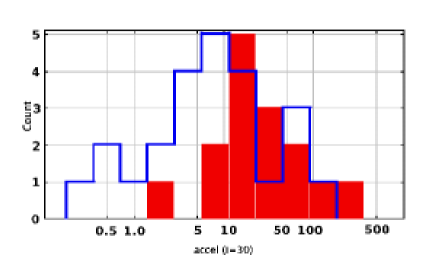
Figure 18: Histogram showing the distribution of radial CO clump acceleration (in $kms^{-1}pc^{-1}$) for clumps with stars (red shaded histogram) and clumps without stars (open histogram). This assumes the same inclination from the plane of the sky for all clumps ($i=30\mbox{\,${}^{\circ}$}$). Clumps with associated stars tend to have the higher apparent acceleration.

Does the presence of a CO clump and envelope associated with the embedded stars necessarily imply a more massive molecular clump was originally present, and that these are the youngest objects in the region? The photoevaporation lifetime of a clump depends on its radius, $r_{c}^{-1.5}$, so compact, denser clumps will survive longer (and will be accelerated more gradually, in the RDI model) than larger, diffuse clumps. Cores containing stars are thought to have a more centrally-peaked structure than starless cores (eg Ward-Thompson et al., 1994), so for the same clump mass, we might expect clumps with a central star would be more centrally-peaked and hence survive longer in the UV environment, compared with a more diffuse starless core. In such circumstances, we would naturally expect to see that many of the longer-lasting clumps will be the ones containing young stars. Rather than the stars still associated with molecular clumps and envelopes being the youngest objects, it would suggest that the presence of the star causes the molecular clump to survive longer in the UV field. Further observations would be of interest to look for other differences between the clumps with and without young stars.

5 Conclusions

A large-scale single-dish imaging survey covering 60$\times$60 pc of the Rosette Nebula and Rosette Molecular Cloud has been carried out with 14 arcsec resolution in the J=3-2 transition of ¹²CO. The resulting datacube has a high spatial dynamic range (the ratio of map size to spatial resolution is $\sim 500$), and reveals the complex and clumpy spatio-velocity structure in the molecular gas throughout the RMC. The following conclusions can be drawn:

• We identify $\sim$2000 clumps with a mass distribution $dN/dM\propto M^{-1.8}$, independent of distance from the central O stars. This is similar to other less disrupted clouds, and suggests the clump mass distribution is not strongly affected by the O stars.

• Comparison of the molecular datacube with optical and infrared images show that all the gas which blue-shifted with respect to the cloud systemic velocity lies in the foreground. Red-shifted gas has no dark absorbing foreground counterpart. The dominant gas motion is therefore expansion from the cluster of O stars.

• The locations and velocities of many of the clumps closest to the O stars can be fit by an 11pc radius expanding ring. This has a dynamical timescale of $\sim 1$ Myr, similar to the nebula age. Stars formed in clumps in this ring are not dynamically bound to the system.

• Most molecular clumps show significant radial velocity gradients, generally radial from the O stars. Velocity gradients tend to be larger for clumps closer to the O stars, and can be explained by acceleration through photodissociation of the cloud edges facing the central stars. However, in one of the clearest cases of an extended clump, the velocity gradient is constant over a distance of $\sim$1.7pc, and it is unclear whether this acceleration mechanism can produce such a constant velocity gradient.

• Comparison with 24-$\mu$m Spitzer images shows many examples of embedded young stars within the accelerating clumps. These are examples of evaporating envelopes, and we find an association between the high velocity gradients and the presence of an embedded star.

• The CO 3-2/1-0 ratio in the clumped gas decreases with distance from the O stars, implying a radial decrease in temperature. Most of the emission from the ¹²CO line is thought to arise from gas on the surface of the externally-heated clumps, with the main energy source being the central O stars.

6 References

Alvarez, C., Hoare, M., Glindemann, A., Richichi, A., 2004, A&A, 427, 505

Aspin, C., 1998, A&A, 335, 1040

Bachiller, R., Fuente, A., Kumar, M.S.N., 2002, A&A, 381, 168

Balog, Z., Muzerolle, J., Rieke, G.H., Su, K.Y.L., Young, E.T., Megeath, S.T., 2007, ApJ, 660, 1532

Berry, D.S., Reinhold, K., Jenness, T., Econonou, F., 2007, in Astronomical Data Analysis Software and Systems XVI, ed. R.A. Shaw, F. Hill & D.J. Bell, ASP Conference Series 376, 425

Bertoldi, F., McKee, C.F., 1990, ApJ, 354, 529

Beuther, H., Schilke, P. Sridharan, T.K., Menten, K.M, Walmsley, C.M., Wyrowski, F., 2002, A&A 383, 892

Blitz, L., Thaddeus, P., 1980, ApJ, 241, 676

Blitz, L., Stark, A.A., 1986, ApJ, 300, L89

Borkin, M., Arce, H., Goodman, A., Halle, M. 2008, in Astronomical Data Analysis Software and Systems XVII, ed. R.W. Argyle, P.S. Bunclark & J.R. Lewis, ASP Conference Series 394, 145

Celnik, W.E., 1985, A&A 144, 171

Covey, K.R., Greene, T.P., Doppmann, G.W., Lada, C.J., 2006, AJ, 131, 512

Dale, J.E., Clark, P.C., Bonnell, I.A., 2007, MNRAS, 377, 535

Drew, J. et al., 2005, MNRAS, 362, 753

Gahm, G.F., Carlqvist, P., Johansson, L.E.B, Mikolic, S., 2006, A & A, 454, 201

Gahm, G.F., Grenman, T., Fredriksson, S., Kristen, H., 2007, AJ, 133, 1795

Galli, D., Walmsley, M., Gonçalves, J., 2002, A&A, 394, 275

Gonzalez-Alfonso, E., Cernicharo, J., 1994, ApJ, 430, L125

Gonzalez-Alfonso, E., Cernicharo, J., Radford, S.J.E., 1995, A&A, 293, 493

Hensberge, H., Pavlovski, K., Verschueren, W., 2000, A&A, 358, 553

Herbig, G.H., 1974, PASP, 86, 604

Hester, J.J. et al., 1996, AJ, 111, 2349

Hester, J.J. & Desch, S.J., 2005, ASP conf. proc. 341, “Chondrites and the Protoplanetary Disk”, ed. Krot, A.N., Scott, E.R.D., Reipurth, B., 107

Heyer, M.H., Carpenter, J.M., Snell, R.L., 2001, ApJ, 551, 852

Heyer, M.H., Williams, J.P., Brunt, C.M., 2006, ApJ, 643, 956

Hills, R.E., et al., (in prep.)

Hovey, G.J., Burgess, T.A., Casorso, R.V., Dent, W.R.F., Dewdney, P.E., Force, B., Lightfoot, J.F., Willis, A.G., Yeung, K.K., 2000, SPIE, 4015, 114

Jenness, T., Cavanah, B., Economou, F., Berry, D.S., 2008, in Astronomical Data Analysis Software and Systems XXX, ed. J. Lewis, R. Argyle, P. Bunclark, D. Evans, & E. Gonazle-Solares, ASP Conference Series (in press)

Kramer, C., Stutzki, J., Röhring, R., Corneliussen, U., 1998, A&A, 329, 249

Krügel, E., 2003, “The Physics of Interstellar Dust”, IOP Publishing, Bristol

Lada, C.J., Gautier, T.N., 1982, ApJ, 261, L161

Lefloch, B., Lazareff, B., 1994, A&A, 289, 559

Lefloch, B., Lazareff, B., 1995, A&A, 301, 522

Li, D., Goldsmith, P.F., Menten, K., 2003, ApJ, 587, 262

Li, J.Z. & Smith, M., 2005, ApJ, 130, 721

Li, J.Z., Smith, M.D., Gredel, R., Davis, C.J., Rector, T.A., 2008, ApJLet, 679, L101

MacLow, M., Klesse, R.S., 2004, Review Modern Physics, 76, 125

McCaughrean, M.J., Andersen, M., 2002, A&A, 389, 513

McKee, C.F., 1989, ApJ, 345, 782

McKee, C.F., Ostriker, E.C., 2007, Ann. Rev. Astr. Astrophys., 45, 565

Oort, J.H. & Spitzer, L., 1995, ApJ, 121, 6

Patel, N.A., Xie, T, Goldsmith, P.F., 1993, ApJ, 413, 593

Patel, N.A., Goldsmith, P.F., Snell, R.L., Hezel, T., Xie, T., 1995, ApJ, 447, 721

Phelps, R.L., Lada, E.A., 1997, ApJ, 477, 176

Phelps, R.L., Ybarra, J.E., 2005, ApJ, 627, 845

Poulton, C.J., Robitaille, T.P., Greaves, J.S, Bonnell, I.A., Williams, J.P., Heyer, M.H., 2008, MNRAS, 384, 1249

Pound, M.W., 1998 ApJ, 493, L113

Rees, N. et al., 2002, SPIE, 4848, 283

Schneider, N., Stutzki, J., Winnewisser, G., Blitz, L., 1996, ApJLet, 468, L119

Schneider, N., Stutzki, J., Winnewisser, G., Block, D., 1998, A&A, 335, 1049

Schneps, M.H., Ho, P.T.P., Barrett, A.H., 1980, ApJ, 240, 84

Smith, H. et al., 2003, SPIE, 4855, 338

Stutzki, J., Güsten, R., 1990, ApJ356, 513

van der Tak, F.F.S., Black, J.H., Schoir, F.L., Jansen, D.J., van Dishoeck, E.F., A&A, 468, 627

Ward-Thompson, D., Scott, P.F., Hills, R.E., Andre, P., 1994, MNRAS, 268, 276

White, G.J., Lefloch, B., Fridlund, C.V.M., Aspin, C.A., Dahmen, G., Minchin, N.R., Huldtgren, M., 1997, A&A, 323, 931

Williams, J.P., Blitz, L, Stark, A.A., 1995, ApJ 451, 252 (W95)

Wu, Y., Wei, Y., Zhao, M., Shi, Y., Yu, W., Qin, S., Huang, M., 2004, A&A 426, 503

Ybarra, J.E., Phelps, R.L., 2004, AJ, 127, 3444