Spectropolarimetry with CRISP at the Swedish 1-m Solar Telescope

Abstract

CRISP (Crisp Imaging Spectro-polarimeter), the new spectropolarimeter at the Swedish 1-m Solar Telescope, opens a new perspective in solar polarimetry. With better spatial resolution (0.13^′′) than Hinode in the Fe I 6302 Å line and similar polarimetric sensitivity reached through postprocessing, CRISP complements the SP spectropolarimeter onboard Hinode. We present some of the data which we obtained in our June 2008 campaign and preliminary results from LTE inversions of a pore containing umbral dots.

1 Introduction

CRISP (CRisp Imaging Spectro-Polarimeter) is a new imaging spectropolarimeter installed at the Swedish 1-m Solar Telescope (SST, Scharmer et al. (2003)) in March 2008. The instrument is based on a dual Fabry-Pérot interferometer system similar to that described by Scharmer (2006). It combines a high spectral resolution, high reflectivity etalon with a low resolution, low reflectivity etalon. It has been designed as compact as possible, i.e., with a minimum of optical surfaces, to avoid straylight as well as possible.

For polarimetric studies, nematic liquid crystals are used to modulate the light. These crystals change state in less than 10 ms, which is faster than the CCD read-out time. A polarizing beam splitter close to the focal plane splits the beam onto two 1024$\times$1024 synchronized CCD’s that measure the two orthogonal polarization states simultaneously. This facilitates a significant reduction of seeing crosstalk in the polarization maps.

A third, synchronized, CCD camera records wide-band images through the prefilter of the Fabry-Pérot system. These images serve as an anchor channel for Multi-Object Multi-Frame Blind Deconvolution (MOMFBD) image restoration (van Noort et al. (2005)) which enables near-perfect alignment between the sequentially recorded polarization and line position images. For more details on MOMFBD processing of polarization data see van Noort & Rouppe van der Voort (2008).

The etalons can sample spectral lines between 510 and 860 nm. The field of view (FOV) is 70^′′$\times$70^′′; the pixel size 0.07^′′/pixel. The instrument has been designed to allow diffraction-limited observation at 0.13^′′ angular resolution in the Fe I 630 nm lines.

2 The June 2008 campaign data and processing

The data displayed here were recorded on June 12, 2008 as part of a campaign during June 2008. The target was a pore (AR 10998) located at S09 E24 ($\mu$=0.79). The field of view was 70^′′$\times$ 70^′′.

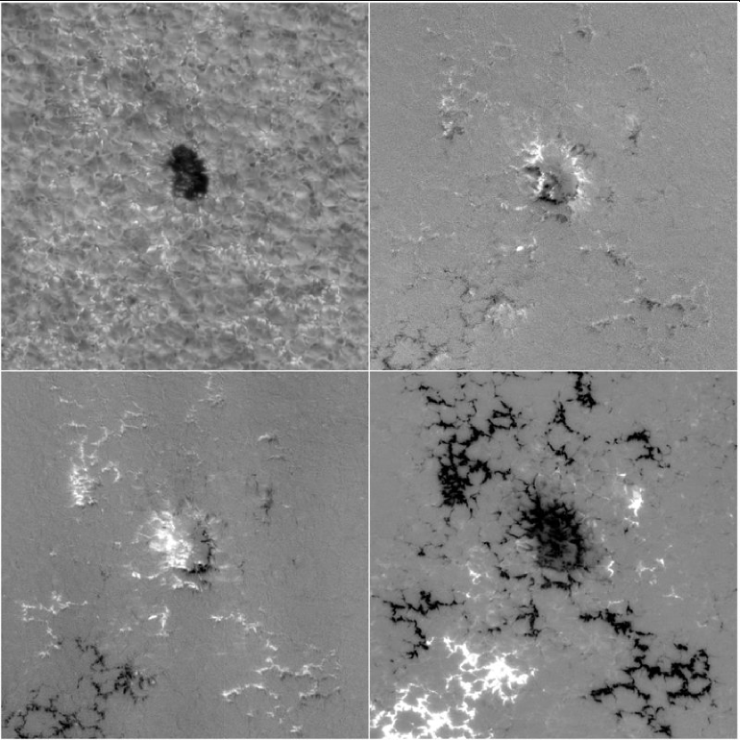
Figure 1: Clockwise: Stokes $I$, $Q$, $V$ and $U$ images taken in the blue wing of Fe I 6302.5 Å at $\Delta\lambda=-48$ mÅ, on June 12, 2008.

The images recorded correspond to complete Stokes measurements at 15 line positions in steps of 48 mÅ, from $-336$ mÅ to +336 mÅ, in each of the Fe I lines, 6301.5 and 6302.5 Å. In addition, images were recorded at one continuum wavelength. Each camera operated at 35 Hz frame rate. For each wavelength and LC state, 7 images were so recorded per camera. Each sequence for subsequent MOMFBD processing consists of about 870 images per CCD (2600 in total), recorded during 30 s. The images were divided into overlapping 64$\times$64 pixel subfields sampling different isoplanaic patches with overlaps. All images from each subfield were then processed as a single MOMFBD set. They were demodulated with respect to the polarimeter and a detailed telescope polarization model. In addition, the resulting Stokes images were corrected for remaining $I$ to $Q$, $U$ and $V$ crosstalk by subtraction of the Stokes continuum images. Figure 1 shows an example of the resulting Stokes images.

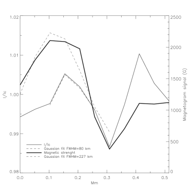
Figure 2: Cut along brightenings in the Stokes I image (thin line) and magnetic field obtained from inversions (thick line). We have fitted a gaussian to the smallest feature we can observe, both in the intensity image and the resulting magnetic field (dotted lines). The fits give us FWHM’s of 80 km for I/Ic and 227 km for the magnetic field.

The theoretical diffraction limit of the SST is $\lambda/D=0.13\hbox{${}^{\prime\prime}$}$ at 6303 Å. We measured the real resolution obtained in our June observations by identifying the smallest intensity feature and fitting a Gaussian to it. Figure 2 shows a cut through a bright point with 80 km FWHM for the Gaussian fit. This value is equivalent to 0.11^′′, which is slightly lower than the theoretical resolution 0.13^′′  but consistent with it, due to the MOMFBD post-processing performed to the data. We estimated the noise level for the Stokes profiles to be around $2\cdot 10^{-3}$ for Stokes Q/I_c, U/I_c and V/I_c.

3 Inversions and results

To derive the atmospheric parameters from the observed Stokes images we use a least-square inversion code, LILIA (Socas-Navarro 2001), based on LTE atmospheres. We assume a one component, laterally homogeneous atmosphere together with stray light contamination. The inversions returns 9 free parameters as a function of optical depth, including the three components of the magnetic field vector (strength, inclination and azimut), LOS velocity and temperature among others. We apply the inversion to both the Fe I 6301.5 and 6302.5 Å lines simultaneously.

Figure 3 shows an example of the inversion of an individual pixel belonging to a bright point. In this particular case the inversion code yielded a field strength of 1100 G, inclination of 25^∘, and LOS velocity of 0.6 km s^-1, (downflow) at $\log(\tau)=-1.5$.

Figure 3: Results from the LILIA inversion of a bright point observed in an intergranular lane. Observed (solid) and fitted (dashed) $I/I_{c}$, $Q/I_{c}$, $U/I_{c}$ and $V/I_{c}$ profiles (upper panels), as well as atmospheric parameters (temperature, magnetic field, inclination and line-of-sight velocity) obtained through the inversion as a function of optical depth (lower panels).

Figures 4 and 5 show maps of the obtained magnetic field strength and line-of-sight (LOS) velocity at different heights. Figure 4 shows a micro-pore as well as brightenings produced by emergent magnetic fields. Ribbons (Berger et al. (2004)) can be distinguished. Upflows are correlated with the positions of the center of the granules, while downflows are correlated with the intergranular lanes, except in those areas where the magnetic field is emerging, in which velocities are lower due to the supression of convection. Figure 5 presents a pore with several umbral dots and structures within. These brighter umbral structures show lower magnetic field strengths than the darker parts of the umbra as well as higher temperatures. Velocities inside the pore tend to be lower than in normal granulation patterns. The velocity field of the umbral structures will be analyzed in a future publication.

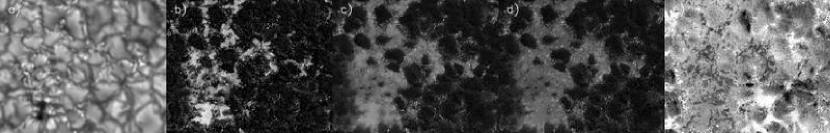
Figure 4: (a) Intensity image of a region containing a micro-pore and intergranular magnetic fields including ribbons and bright points. (b) (c) and (d): Mmagnetic field strength maps resulting from the inversion at log($\tau$)=0, -1.5 and -2 respectively. (e) LOS velocity map at log($\tau$)=-2. Downflows are observed in the intergranular lanes, while upflows are observed in the center of granules. The FOV is 14^′′$\times$ 10^′′.

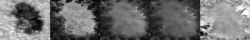
Figure 5: (a) Intensity image of a region containing a sunspot. Umbral dots and other structures can be identified. (b), (c) and (d): magnetic field strength maps resulting from the inversion at $\log(\tau)=0$, $-1.5$, and $-2$, respectively. (e) LOS velocity map at $\log(\tau)=-2$. The FOV is 10^′′$\times$ 10^′′.

4 Discussion

We have presented the first LTE inversions based on data obtained with the CRISP imaging spectropolarimeter, used with the 1-m SST. The spatial resolution of the Stokes data presented here represents a major improvement compared to other ground-based data and even to the recent Hinode data. We have shown here both the capabilities of the CRISP instrument and of the inversion code applied to this data. We expect to make use of such capabilities for exploring in detail the umbral dots and other structures found in the micro-pore present on June 12, 2008.